19th century glacier representations and fluctuations in the central and western European Alps: An interdisciplinary approach
←
→
Page content transcription
If your browser does not render page correctly, please read the page content below
Available online at www.sciencedirect.com

                                             Global and Planetary Change 60 (2008) 42 – 57
                                                                                                             www.elsevier.com/locate/gloplacha

 19th century glacier representations and fluctuations in the central
    and western European Alps: An interdisciplinary approach
                                   H.J. Zumbühl ⁎, D. Steiner ⁎, S.U. Nussbaumer
                             Institute of Geography, University of Bern, Hallerstrasse 12, CH-3012 Bern, Switzerland
                                       Received in revised form 22 August 2006; accepted 24 August 2006
                                                        Available online 22 February 2007

Abstract

    European Alpine glaciers are sensitive indicators of past climate and are thus valuable sources of climate history. Unfortunately,
direct determinations of glacier changes (length variations and mass changes) did not start with increasing accuracy until just before
the end of the 19th century. Therefore, historical and physical methods have to be used to reconstruct glacier variability for
preceeding time periods.
    The Lower Grindelwald Glacier, Switzerland, and the Mer de Glace, France, are examples of well-documented Alpine glaciers
with a wealth of different historical sources (e.g. drawings, paintings, prints, photographs, maps) that allow reconstruction of
glacier length variations for the last 400–500 years. In this paper, we compare the length fluctuations of both glaciers for the 19th
century until the present.
    During the 19th century a majority of Alpine glaciers – including the Lower Grindelwald Glacier and the Mer de Glace – have
been affected by impressive glacier advances. The first maximum extent around 1820 has been documented by drawings from the
artist Samuel Birmann, and the second maximum extent around 1855 is shown by photographs of the Bisson Brothers. These
pictorial sources are among the best documents of the two glaciers for the 19th century.
    In addition to an analysis of historical sources of the 19th century, we also study the sensitivity of the Lower Grindelwald
Glacier to climate parameters (multiproxy reconstructions of seasonal temperature and precipitation) for an advance and a retreat
period in the 19th century using a new neural network approach. The advance towards 1820 was presumably driven by low summer
temperatures and high autumn precipitation. The 1860–1880 retreat period was mainly forced by high temperatures. Finally, this
nonlinear statistical approach is a new contribution to the various investigations of the complex climate–glacier system.
© 2007 Elsevier B.V. All rights reserved.

Keywords: glacier fluctuations; historical sources; sensitivity analysis; neural network

1. Introduction                                                               deduced from natural archives and a wealth of
                                                                              documentary evidence (e.g. Zumbühl and Holzhauser,
   During the 19th century impressive glacier advances                        1988; Maisch et al., 1999). In general, historical records
affected the majority of the Alpine glaciers. This can be                     give a detailed picture of glacial fluctuations and allow
                                                                              studying glacier history further back in time than would
                                                                              be possible from direct measurements alone (e.g.
 ⁎ Corresponding authors. Tel.: +41 31 631 85 51; fax: +41 31 631 85 11.      Holzhauser et al., 2005). For instance, empirical quali-
    E-mail addresses: zumbuehl@giub.unibe.ch (H.J. Zumbühl),                  tative and/or quantitative data on the length, area and
steiner@giub.unibe.ch (D. Steiner).                                           volume of glaciers can be derived from these sources.
0921-8181/$ - see front matter © 2007 Elsevier B.V. All rights reserved.
doi:10.1016/j.gloplacha.2006.08.005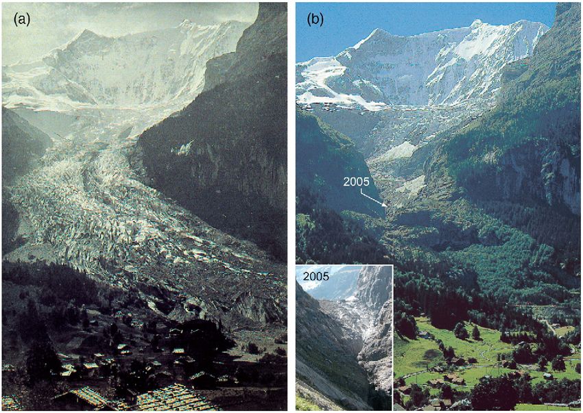
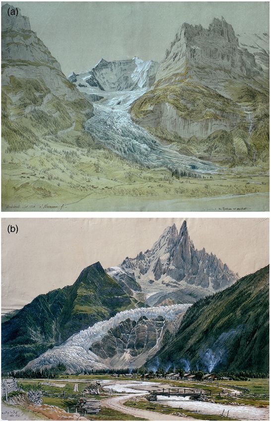
H.J. Zumbühl et al. / Global and Planetary Change 60 (2008) 42–57                                         43

   This study focuses on two well-documented Alpine                          we present different kinds of historical pictorial sources
glaciers, the Lower Grindelwald Glacier, Switzerland,                        (drawings and photographs) that together document the
and the Mer de Glace, France (Fig. 1). For both glaciers                     19th century glacier maximum extents around 1820

Fig. 1. Geographical location of study sites: (a) the Grindelwald region with the Lower Grindelwald Glacier, (b) the Mont Blanc region with the Mer
de Glace.
44                             H.J. Zumbühl et al. / Global and Planetary Change 60 (2008) 42–57

and 1855. Samuel Birmann (1793–1847), an important                of the Mont Blanc (France). The topography and some
Swiss landscape artist, portrayed the Lower Grindel-              landmark locations of these two glaciers are shown in
wald Glacier and the Mer de Glace at their first                  Fig. 1.
maximum extent around 1820 in detailed drawings of                    The Lower Grindelwald Glacier (46°35′ N, 8°05′ E)
their glacier snouts. The Bisson Brothers, famous                 is a valley glacier, 8.85 km long and covering a surface
photographers of that time, made pictures of the two              of 20.6 km2. Ischmeer in the east and the Bernese
glaciers at their second maximum extent around 1855,              Fiescher Glacier in the west join to form the tongue of
again including detailed views of their glacier snouts.           the Lower Grindelwald Glacier (Fig. 1a). The main
Therefore, the historical sources of the two glaciers             contribution of ice presently originates from the Bernese
allow comparison of these extraordinary high-quality              Fiescher Glacier (Holzhauser and Zumbühl, 1996;
glacier representations at their maximum extent. It               Schmeits and Oerlemans, 1997). The approximated
must be noted that the change of glacier representation           equilibrium line altitude (ELA), derived from digital
techniques from drawings to photographs demonstrates              elevation models (DEMs), is at 2640 m a.s.l. The glacier
also the changing view on glaciers from the magic                 today terminates at 1297 m a.s.l. in a narrow gorge so
to the scientific (Haeberli and Zumbühl, 2003; Steiner            that reliable observations are difficult to obtain (data
et al., in press).                                                from 2004: Steiner et al., in press).
   Furthermore, the 19th century provides also an                     The Mer de Glace (45°54′ N, 8°57′ E) sensu lato is a
opportunity to analyze the climatic conditions of the             compound valley glacier, 12.0 km long and covering a
last widespread glacier advance and the following                 surface of 31.9 km2 (without including Glacier de
retreat. This is done by connecting new gridded                   Talèfre). The glacier is fed by several tributaries with the
reconstructions of temperature and precipitation (Luter-          Glacier du Géant being the most important one (Fig. 1b).
bacher et al., 2004; Pauling et al., 2006) with the data          Since the 1931–1969 retreat, the Glacier du Talèfre is
of length fluctuations of the Lower Grindelwald                   separated from the main ice stream. The Mer de Glace
Glacier. Because the climate–glacier relation is, in              sensu stricto refers to the lowest approximately 5 km
part, nonlinear (Steiner et al., 2005), we suggest a new          of the ice stream, forming the glacier tongue beneath
statistical nonlinear approach based on a neural                  Montenvers. The ELA is situated at around 2775 m a.s.l.,
network to investigate the climate–glacier system, i.e.           and the glacier today terminates at 1467 m a.s.l. (data
to study the meteorological conditions which led to a             from 2001: Nussbaumer et al., in press).
glacier advance or retreat. In a sensitivity analysis that            The Bernese Alps is a group of mountain ranges in
explores the significance of climatic inputs to the               the central part of the Alps drained by the river Aare and
glacier system we evaluate the relevant climatic                  its tributary Saane in the north, and the Rhône in the
variables that caused the advance towards 1820 and                south and the Reuss in the east. The northern part of the
the rapid retreat of the Lower Grindelwald Glacier after          Bernese Alps, including the Lower Grindelwald Glacier,
1860.                                                             is exposed to the westerlies and receives maximum
   In this paper, we compare the length fluctuations of           precipitation during summer, with low variability. The
the Lower Grindelwald Glacier and the Mer de Glace                mean annual temperature at Grindelwald (1040 m a.s.l.),
since 1800. Since this approach is descriptive, we also           located approximately 3 km from the glacier front of the
present a neural network model to explore potential               Lower Grindelwald Glacier, was 6.7 °C during the
climate forcings to explain glacier length fluc-                  1966–1989 period. The mean temperature during the
tuations with the Lower Grindelwald Glacier. There-               accumulation season (October–April) and ablation
fore, the analysis of historical sources provides a               season (May–September) during the 1966–1989 period
framework for which we can test the relative im-                  was 2.3 °C and 12.9 °C, respectively.
portance of climate variables forcing glacier advance                 The mean annual precipitation during the 1961–1990
and retreat.                                                      period was 1428 mm with precipitation during the
                                                                  accumulation season (October–April) and ablation
2. Data and methods                                               season (May–September) of 720 mm and 708 mm,
                                                                  respectively (data from the online database of Meteo-
2.1. Study area                                                   Swiss). Because of high precipitation (locally exceeding
                                                                  4000 mm per year), the Bernese Alps have a relative low
   Our study focuses on the Lower Grindelwald                     glacier equilibrium line altitude and is the heaviest
Glacier, located in the northern Bernese Alps (Switzer-           glacierized region in the Alps. Both the glacier with the
land), and the Mer de Glace, located on the north face            lowest front (Lower Grindelwald Glacier) and the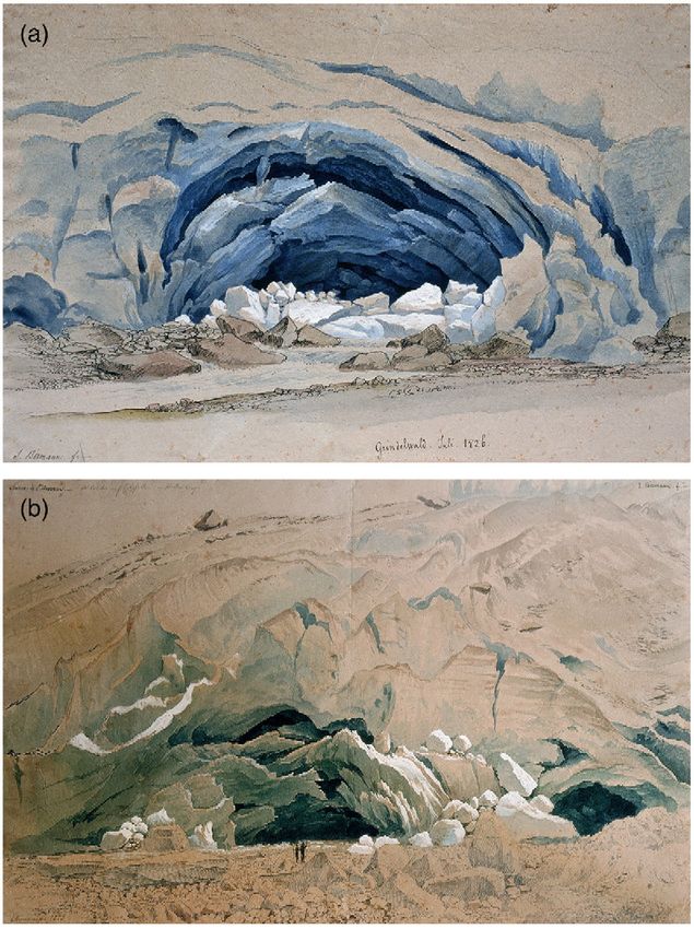
H.J. Zumbühl et al. / Global and Planetary Change 60 (2008) 42–57                         45

largest glacier of the Alps (Great Aletsch Glacier) are           et al., 2005). The density of historical material prior to
located within this region (Kirchhofer and Sevruk,                1800 highly depends on the elevation of the tongue and
1992; Imhof, 1998).                                               the relationship between settlements and cultivated land
    Due to the extraordinary low position of the terminus         and the glacier advances.
and its easy accessibility, the Lower Grindelwald                    Historical data have to be considered carefully and
Glacier is one of the best-documented glaciers in the             local circumstances need to be taken into account. The
Swiss Alps, and likely in the world. The cumulative               evaluation of historical sources, the so-called historical
length fluctuations of the Lower Grindelwald Glacier,             method, has to fulfill some conditions in order to
derived from documentary evidence, covers the period              obtain reliable results concerning former glacier
1535–1983 including the two well-known glacier                    extents (Zumbühl and Holzhauser, 1988): Firstly, the
maxima about 1600 and 1855/56 (Zumbühl, 1980;                     dating of the document has to be known or recon-
Holzhauser and Zumbühl, 1996, 2003).                              structed. This often includes labour-intensive archive
    The Mont Blanc mountain range (Fig. 1) extends                work. Secondly, the glacier and its surroundings have
50 km from Martigny (Switzerland) in the northeast to             to be represented realistically and topographically
St. Gervais (France) in the southwest, forming the                correct which requires certain skills of the correspond-
watershed between France and Italy and separating the             ing artist. In addition, the artist's topographic position
uppermost catchment areas of the Rhône and Po rivers.             should be known; prominent features in the glacier's
On the French side of the mountain range, the upper               surroundings such as rock steps, hills or mountain
Arve river flows down the deep trough of Chamonix,                peaks facilitate the evaluation of historical documen-
with several glaciers (Glacier du Tour, Glacier d'Ar-             tary data.
gentière, Mer de Glace, Glacier des Bossons) draining                Note that for both the Lower Grindelwald Glacier,
into this river. Climate in the valley of Chamonix is             and the Mer de Glace, there is a wealth of historical
typical for the western Alps and comparable to the                (pictorial) documents which has been evaluated.
Grindelwald area, although slightly drier. Annual                 Probably the best example of a glacier curve derived
temperature of the Chamonix meteorological station                from historical sources is the series of cumulative length
(1054 m a.s.l.) is 6.6 °C for the 1935–1960 period,               changes of the Lower Grindelwald Glacier (Zumbühl,
the annual precipitation amounts to 1262 mm for the               1980; Zumbühl et al., 1983).
1934–1962 period (Wetter, 1987).
    The Mer de Glace is the longest and largest glacier           2.3. Sensitivity analysis by neural networks
of the western Alps. During the Little Ice Age (LIA),
the period lasting a few centuries between the Middle                The evaluation of historical data gives insight into
Ages and the warming of the first half of the 20th                the change in glacier length over time without showing
century (Grove, 2004), the glacier nearly continuously            the climatic driving factors which presumably affected
reached the bottom of the valley of Chamonix at                   these glacier changes. To investigate the relationship
1000 m a.s.l. This lowest part of Mer de Glace was                between the meteorological conditions and variations
called Glacier des Bois which today has completely                of glaciers many studies have been carried out. For
melted away. Similar to the Lower Grindelwald Glacier,            instance, regression techniques with different numbers
the Mer de Glace has been well observed by scientists,            and types of predictors have often been used (Oerle-
artists, and travellers since the beginning of alpinism,          mans and Reichert, 2000, and references therein).
leading to a large number of historical documentary               Besides these classical methods that commonly use
data.                                                             linear assumptions, neural network models (NNMs)
                                                                  have become popular for performing nonlinear re-
2.2. Historical sources in glaciology                             gression and classification (Steiner et al., 2005, and
                                                                  references therein). Because glacier length is a
   If sufficient in quality and quantity, written docu-           complex function dependent on climate, time, glacier
ments and pictorial historical records (paintings,                geometry and other factors, it may be well-suited to
sketches, engravings, photographs, chronicles, topo-              nonlinear model approaches. Therefore, modelling re-
graphic maps, reliefs) provide a detailed picture of              sults can complement the historical analysis in order
glacier fluctuations over the last few centuries. Using           to give a better picture of how, and why the glacier has
these data, we can achieve a resolution of decades or, in         reacted.
some cases, even individual years of ice margin                      Inspired by the human brain, a neural network (NN)
positions (Zumbühl and Holzhauser, 1988; Holzhauser               consists of a set of highly interconnected units, which
46 H.J. Zumbühl et al. / Global and Planetary Change 60 (2008) 42–57
process information as a response to external stimuli. A and the remaining 25% for validation (Walter and
neural network is thus a simplistic mathematical Schönwiese, 2003).
representation of the brain that emulates the signal A typical NN model consists of three layers: input,
integration and threshold firing behaviour of biological processing and output layers (Fig. 2). The input to an
neurons by means of mathematical equations. NN model is a vector of elements xk, where the index k
The most widely used NN models are the feed- stands for the number of input units in the network. In
forward neural networks (Rumelhart et al., 1986). this study two new gridded (0.5° × 0.5° resolution)
Their applications cover a broad field of the envi- multiproxy reconstructions of seasonal temperature
ronmental sciences including meteorology and clima- (Luterbacher et al., 2004) and precipitation fields
tology. Some examples of recent applications using (Pauling et al., 2006) from 1500–2000 for European
NN include the detection of anthropogenic climate land areas were used as input data. These inputs serve as
change (Walter and Schönwiese, 2002, 2003) and the climatic driving factors to the glacier system. Before
study of an Alpine glacier mass balance (Steiner et al., processed the inputs are weighted with weights wjk
2005). where j represents the number of processing units, to
In this study the standard NN model, the Back- give the inputs to the processing units.
propagation Network (BPN), was applied (Rumelhart Using too few/many processing units can lead to
et al., 1986). This network architecture is based on a underfitting/overfitting problems because the simulation
supervised learning algorithm to find a minimum cost results are highly sensitive to the number of processing
function. Because this approach bears a certain risk of units and learning parameters. Therefore a variety of
overfitting, the data have to be separated into a training BPNs must be checked to obtain robust results.
and a validation subset. The actual ‘learning’ process For the simulation of the glacier length variations of
of the network is performed on the training subset the Lower Grindelwald Glacier we used six potential
only, whereas the validation subset serves as an input units as forcings (Temp_MAM, Temp_JJA,
independent reference for the simulation quality. This Temp_SON, Prec_DJF, Prec_MAM, Prec_SON), each
technique is called Cross-Validation (Stone, 1974; of them have been stepwise shifted so that all lags
Michaelsen, 1987). When applying NN models to a between 0 and 45 years are considered to account for the
nonstationary time series, as in this approach, the uncertain and changing reaction time of this glacier. As
training subset includes the full range of extremes in target function we apply the curve of length variations of
both predictors and predictands. Otherwise, the algo- the Lower Grindelwald Glacier. In this manner the NN
rithm will fail during the validation process if con- model will use those shifted input series that explain the
fronted with an extreme value that was not part of the glacier length variations. Hence, there are 46·6 = 276
training subset. We used 75% of all data for training input units (climate variables), 138 processing units in 1
Fig. 2. An example of a simplified 3-layer k–j–1 BPN architecture. The concept of the backpropagation training algorithm is shown by several arrows
(from Steiner et al., 2005). Note that in our study the input layer consists of the climatic inputs and the output layer represents the glacier length.H.J. Zumbühl et al. / Global and Planetary Change 60 (2008) 42–57 47
processing layer and the length fluctuations as output with the error made when restricting the input of interest
unit. This neural network architecture is abbreviated as to the average value. Thus, the greater the increase in the
276-138-1. error function upon restricting the input, the greater the
After weighting and adding of the inputs, the results importance of this input in the output (e.g. Wang et al.,
were passed to nonlinear activation functions (e.g. 2000). In this study we kept one seasonal temperature or
sigmoid functions) in each processing unit (processing precipitation input constant while the other inputs were
layer in Fig. 2). These functions produced the output of allowed to fluctuate. The observed error of glacier
the processing layer. The outputs of the processing units response gave us indications of its sensitivity to the
are fed to the output layer where they are again weighted input that was constant.
with the weights Wij. The use of a second activation
function will finally produce the output of the network 3. Results
(output layer in Fig. 2).
The purpose of training an NN model is to find a set 3.1. Two glaciers drawn by the artist Samuel
of coefficients that reduces the error between the model Birmann — The first advance in the 19th century
outputs and the given test data y(xk). This is usually
done by adjusting the weights Wij and wjk to minimize On the pencil watercolor drawing by Samuel
the least square error. One way to adjust these weights Birmann (1793–1847) made in September 1826 (Fig.
is error backpropagation. The backpropagation training 3a), the marked fanshaped tongue – the “Schweif” or
consists of two passes of computation: a forward pass tail (covering the Schopfrocks) – of the Lower
and a backward pass. In the forward pass an input Grindelwald Glacier extends far down into the valley.
vector is applied to the units in the input layer. The The skyline of the drawing is dominated by the
signals from the input layer propagate to the units in Mettenberg (left), the Fiescherhorn (center background)
the processing layer and each unit produces an output. and the Hörnligrat (right; see Fig. 1). In the forefield of
The outputs of these units are propagated to units in the glacier (right) we can clearly recognize a complex
subsequent layers. This process continues until the moraine system. The wooden area between the ice front
signals reach the output layer where the actual response and the moraine walls shows that the Lower Grindel-
of the network to the input vector is obtained. During wald Glacier reached a bigger extension in earlier times
the forward pass the weights of the network are fixed. (around 1600; Zumbühl, 1980), and that the 1814–
During the backward pass (see dashed arrows in Fig. 1820/22 advance amounts to 450–520 m, approxi-
2), on the other hand, the weights are all adjusted in mately 75–150 m behind the greatest LIA extension
accordance with an error signal that is propagated around 1600.
backward through the network against the initial In this context it must be noted that Samuel Birmann
direction. from Basel was “the most important Swiss romantic of
As mentioned above, this network architecture still topographic landscape artists” (Zumbühl, 1997). We
bears the risk of being stuck in local minima on the error know of approximately 100 views of glaciers, all
hypersurface. To reduce this risk, conjugate gradient produced within 20 years (1815–1835). The drawings
descent was used in this study. This is an improved are all of an outstanding topographic quality and due to
version of standard backpropagation with accelerated the very wide angle often used in his views, they are
convergence. A detailed description of this technique comparable to photographs, in many ways even superior
can be found in Steiner et al. (2005). to them.
A second uncertainty in the BPN simulation is related Among this unique collection of glacier views by
to the fact that the identified minimum is dependent on Samuel Birmann, there is also a pencil watercolor
the starting point on the error hypersurface. To reduce drawing of the Mer de Glace from 1823 (Fig. 3b). The
this kind of uncertainty, the BPN was performed 30 drawing shows the impressive peaks of the Aiguille
times, each time only varying the starting point on the Verte and les Drus (skyline) and the ice flow of the
error hypersurface. Finally, the average of the 30 model Glacier des Bois that terminated near the village of les
results has been analyzed. Bois (roof and chimneys with smoke) in the valley
Sensitivity analysis using neural networks is based bottom. Similar to Grindelwald with the Schopfrocks
on the measurements of the effect that is observed in the the ice front terminates in a rocky zone, Rochers des
output layer due to changes in the input data. A common Mottets (middleground between village and peaks). A
way to perform this analysis consists of comparing the close look reveals also the moraines of Côte du Piget
error made by the network from the original patterns (left).48 H.J. Zumbühl et al. / Global and Planetary Change 60 (2008) 42–57
Fig. 3. The Swiss artist Samuel Birmann (1793–1847) portrayed (a) the Lower Grindelwald Glacier in September 1826 (39.2 × 49.7 cm; pencil, pen,
watercolor, bodycolor), (b) the Mer de Glace in August 1823 (44.3 × 58.9 cm; pencil, pen, watercolor, bodycolor). Kupferstichkabinett,
Kunstmuseum Basel. Photographs by Heinz J. Zumbühl.
In the “Souvenirs de la vallée de Chamonix”, a the valley approximately 560 m (Nussbaumer et al., in
precious artbook with aquatints (colorprints), Samuel press). This amount is similar to Grindelwald, but the
Birmann writes to view No. 21 “Glacier des Bois”: “In advance took place in a shorter time. In 1821, the Mer de
1821, the glacier advanced until twenty feet to a house Glace reached the largest extension in the 19th century,
of the village [les Bois]; so the people prepared to leave comparable to the Rosenlaui Glacier in 1826 (Zumbühl
their homes, but this time, the glacier respected his and Holzhauser, 1988), but different to the Lower
limits, and since then he started to melt back slowly” Grindelwald Glacier which reached its peak in 1855/56.
(translated from Birmann, 1826). The advance, starting The same artist offers us also detailed views of the
around 1800 and ending in 1821, pushed the ice front in fronts of the glaciers mentioned with two huge glacierH.J. Zumbühl et al. / Global and Planetary Change 60 (2008) 42–57 49
snouts in the valley bottom. Firstly, the Mer de Glace ques, from drawings and prints to the much more precise
in 1823 with the source of the l'Arveyron is shown in first photographs.
Fig. 4b, and secondly, the Lower Grindelwald Glacier The probably first photograph of the Lower
in 1826 with the source of the Lütschine is shown in Grindelwald Glacier was taken by the Bisson Brothers
Fig. 4a. (Fig. 5a). Louis Auguste Bisson “the older” (1814–
1876), originally architect, and his brother Auguste
3.2. Two glaciers from the same photographer family Rosalie Bisson, “the younger” (1826–1900), originally
(the Bisson Brothers) — The second mid 19th century painter, founded in 1840 a company for producing
advance daguerreotypes. Later, they became very famous for
their impressive photographic views of the Mont Blanc.
The mid 19th century was in many ways a very These views were made for the French emperor
interesting time. Firstly, it brought the second advance Napoléon III.
and for many glaciers the maximum extension in the One of the big challenges using historical pictorial
19th century. Secondly, this time brought also a views in glacier reconstructions is the precise dating of
revolutionary change of glacier representation techni- the data sources, especially for photographs. Thanks to
Fig. 4. Samuel Birmann also produced detailed views of the glacier snouts of (a) the Lower Grindelwald Glacier in July 1826 (30.3 × 45.2 cm; pencil,
pen, watercolor, bodycolor) and (b) the Mer de Glace in 1823 (30.1 × 45.7 cm; pencil, pen, watercolor, bodycolor). Kupferstichkabinett,
Kunstmuseum Basel. Photographs by Heinz J. Zumbühl.50 H.J. Zumbühl et al. / Global and Planetary Change 60 (2008) 42–57 Fig. 5. Photographs from the Bisson Brothers showing (a) the Lower Grindelwald Glacier in 1855/56 (34.2 × 44.4 cm) and (b) the Mer de Glace in 1854 (34.1 × 45.4 cm). Alpine Club Library, London. Photographs by Heinz J. Zumbühl. the growing interest for this subject during the last ice front. Starting from a high ice level just down in the twenty years, we now have more possibilities to address valley (a big part of the “Schweif” existed) the front of this topic. For the probably oldest photograph of the the Lower Grindelwald Glacier advanced 75–150 m Lower Grindelwald Glacier, there are three proofs: between 1839 (1843) and 1855/56 (Zumbühl, 1980). Firstly, the black ink stamp “Bisson frères” at the edge of In 1849, John Ruskin made the oldest photo known the photo (this black stamp was only used from 1854– from the Mer de Glace in the area of Montenvers. Five 1857; see Chlumsky et al., 1999), secondly, travels to years later, in 1854, the Bisson Brothers took a photo of Switzerland in 1855/56 (Chlumsky et al., 1999), and the Glacier des Bois in the valley bottom, maybe the first thirdly, an advertisement of the Bisson Brothers in the one from this site (de Decker Heftler, 2002; Fig. 5b). journal “L’Artiste” (14 December 1856) give us strong The frontal zone of the Mer de Glace advanced approx- evidence that the photograph was taken in 1855/56, imately 290 m from 1842 to 1852 (Nussbaumer et al., during the mid 19th century maximum extension. in press). Additionally, the photograph shows the glacier during Comparable to previous views we can now look at late summer/early autumn season as there is a snow free the impressive glacier snouts in the valley bottom in
H.J. Zumbühl et al. / Global and Planetary Change 60 (2008) 42–57                                        51

detail. In 1861, a partially collapsed snout of the Lower                   1994). In 1859, the archlike snout of the Mer de Glace
Grindelwald Glacier with the Lütschine (Fig. 6a) was                        with the source of the Arveyron river was still intact on
photographed by Adolphe Braun (1812–1877; Kempf,                            the photo of the Bisson Brothers (Fig. 6b).

Fig. 6. (a) The snout of the Lower Grindelwald Glacier in 1861 (8.1 × 14.4 cm; cut-out). Stereograph “1109 Source de la Lutschine” by Adolphe
Braun (1812–1877). Private Collection of Jaroslav F. Jebavy, Geneva. (b) The snout of the Mer de Glace in 1859 (23.2 × 39 cm). Photograph “Source
de l’Arveyron” by the Bisson Brothers. Private collection of J. and S. Seydoux; Musée Savoisien, Chambéry (Exposition 2002).
52                                    H.J. Zumbühl et al. / Global and Planetary Change 60 (2008) 42–57

3.3. The history of the two glaciers from the 19th century                   bigger than the 1820/22 extent, while the Mer de Glace
until today — Variations of length based on historical                       had the second peak of the 19th century in 1852/53
pictorial and written sources/documents                                      which was less pronounced than in 1821.
                                                                                Finally, after the end of the LIA both glaciers retreated
    Historic length variation of the Lower Grindelwald                       dramatically. The Lower Grindelwald Glacier melted
Glacier (Fig. 7) belongs to the world's best-documented                      back approximately 1000 m during the 1860–1880
and longest ones of its kind thanks to a unique wealth of                    period, the Mer de Glace showed a retreat of approxi-
historic picture sources (Zumbühl, 1980; Zumbühl et al.,                     mately 900 m during the 1867–1878 period.
1983; Oerlemans, 2005). Since the 1980s we were able
to collect new photographic documents which provide                          3.4. Precipitation and temperature significance for the
more detailed views of the mid 19th century ice margins                      glacier variations in the 19th century
(Steiner et al., in press).
    The cumulative length curve of the Mer de Glace                             Here we explore the climatic forcings that may have
(Fig. 7) is the result of the studies of Mougin (1912) and                   been instrumental in the glacier fluctuations described
Wetter (1987). Based on a huge collection of historical                      above. Glacier mass balance and subsequent frontal
pictorial records, partly never studied before, Nussbau-                     response is influenced by climate, mainly temperature
mer et al. (in press) refined the curve of length variations                 during the ablation season (summer) and precipitation
of the Mer de Glace.                                                         during the accumulation season (winter). In an attempt
    Comparing the cumulative length curves of the Lower                      to find consistency between glacier advances and both
Grindelwald Glacier and the Mer de Glace for the 19th                        temperature and precipitation reconstructions, we com-
century yields the following results (Fig. 7): Both                          pared the Lower Grindelwald Glacier (Switzerland) with
glaciers show a rapid advance at the beginning of the                        precipitation reconstructions by Pauling et al. (2006)
19th century. The Lower Grindelwald Glacier reaches its                      and temperature reconstructions by Luterbacher et al.
first maximum extent in 1820/22, the Mer de Glace in                         (2004).
1821. In the following years both glaciers remain in or                         Before feeding the BPN, the input data was
near the valley bottom, implying no significant retreat.                     standardized to their mean and standard deviation over
    Then, in 1855/56 the Lower Grindelwald Glacier                           the whole training/verification period 1535–1983 so
reached its second peak of the 19th century which was                        that temperature and precipitation are comparable (for a

Fig. 7. Cumulative length variations of the Lower Grindelwald Glacier (solid line; Zumbühl, 1980; Holzhauser and Zumbühl, 1996, 2003; Steiner
et al., in press) and the Mer de Glace (dashed line; data 1911–2003 from the Laboratoire de Glaciologie et Géophysique de l'Environnement LGGE;
Nussbaumer et al., in press) from 1800 onwards, relative to the 1600s maximum extent. The points on the curves indicate the ice margin locations as
depicted in Figs. 3–6 and 9–10.
H.J. Zumbühl et al. / Global and Planetary Change 60 (2008) 42–57 53 robust NN performance). As explained before, each therefore glacier length. So, these two time series are not climate input has been stepwise shifted in time so that all used as input variables (Oerlemans and Reichert, 2000; lags between 0 and 45 years have been used. This was Reichert et al., 2001; personal communication by done to account for the varying reaction time of the Johannes Oerlemans, University of Utrecht, 10.8.2005). glacier. The lag time has been fixed according to Schmeits After training the BPN, one input has been set to its and Oerlemans (1997), and Haeberli and Hoelzle (1995), mean and the rest of the inputs to their real values. The respectively, which calculated a response time for trained model has been fed with this new pattern. By the Lower Grindelwald Glacier of 34–45 years, and comparing the network error of the original model with 20–30 years, respectively. Furthermore, it must be noted the error resulting from the new pattern, we can establish that the reaction to climate at the glacier snout can also be a relative importance of the changed input variable. This more immediate in some situations, e.g. after runs of cool procedure is repeated for each input variable. summers (Matthews and Briffa, 2005). Fig. 8 shows a boxplot describing the relative To investigate the relative importance of the importance of the input data for the 1810–1820 advance influential factors we performed a sensitivity analysis and 1860–1880 retreat period of the Lower Grindelwald using neural networks based on winter (Prec_DJF), Glacier (Zumbühl, 1980; Zumbühl et al., 1983; spring (Prec_MAM) and autumn precipitation (Pre- Holzhauser and Zumbühl, 2003). Each boxplot is c_SON) as well as spring (Temp_MAM: Xoplaki et al., based on the average outputs of 30 model runs with 2005), summer (Temp_JJA) and autumn temperature different lags as input to reduce the effect of falling into (Temp_SON: Xoplaki et al., 2005) as input variables of local minima (Steiner et al., 2005). This resulted in an the Backpropagation Neural Network (BPN) (Fig. 2). assessment of the relative importance of the input An analysis of the Seasonal Sensitivity Characteristics variables. (SSCs) of the Lower Grindelwald Glacier showed that The 1810–1820 advance (Fig. 8a), which marks the summer (JJA) precipitation and winter (DJF) tempera- beginning of the mid 19th century maximum glacier ture do not lead to a strong response in mass balance and extent, was presumably driven by low summer tempera- Fig. 8. Relative importance of climate input variables to length fluctuations of the Lower Grindewald Glacier (Switzerland) for the following periods: (a) 1810–1820 advance period, (b) 1860–1880 retreat period. For each input variable to the neural network the median, the first and third quartile (lower/upper hinge) and a 95% confidence interval for the median (lower/upper whisker) of the 30 model runs are given.
54 H.J. Zumbühl et al. / Global and Planetary Change 60 (2008) 42–57
tures (more than 80% relative input importance) and graphs by the Bisson Brothers and others are both
high autumn precipitation. Note that in this case the outstanding examples of glacier representations from
variability of the relative importance is lower compared the last part of the Little Ice Age (LIA). Pictorial sources
to other advance periods (not shown). Furthermore, this therefore provide insight into glacier changes as well as
advance shows specifically the expected pattern of an on changing views on glaciers. As a consequence, we are
advancing Alpine glacier: Low summer temperatures able to do both comparisons of glacier representa-
during the advance period hinder ablation making tions and a qualitative analysis of glacier variations.
glacier advances possible. Above normal (autumn) pre- Figs. 9 and 10 show the enormous glacier changes that
cipitation leads to a positive mass balance in the accu- have occurred since the last LIA glacier maximum
mulation area. This is a prerequisite for later advances of extent.
the glacier snout. After analyzing new documentary data, we show that
It is not surprising that the 1860–1880 retreat period the series of length fluctuations of the Lower Grindel-
was mainly driven by high temperatures. High spring wald Glacier and the revised curve of the length fluc-
temperatures and decreasing autumn precipitation could tuations of the Mer de Glace are very similar – despite
have been the cause for the 1860–1880 retreat (Fig. 8b). the big spatial distance between the glaciers.
The analysis of historical sources and the hereby
4. Discussion and conclusions derived quantitative data are the prerequisite to study
the connection between climatic driving factors and
The Lower Grindelwald Glacier and the Mer de glacier changes. In a new nonlinear neural network
Glace are among the best-documented glaciers with approach which has been successfully applied to
different kinds of historical sources. The high-quality analyze the sensitivity of the Lower Grindelwald
drawings by Samuel Birmann and the first photo- Glacier to different climate parameters, we show that
Fig. 9. (a) The Lower Grindelwald Glacier 1858 in the valley floor, 2–3 years after the maximum extent in 1855/56 (31.9 × 25.2 cm). Photograph by
Frédéric Martens (1806–1885). Alpine Club Library, London. Photograph by Heinz J. Zumbühl. (b) The Lower Grindelwald Glacier 1974.
Photograph by Heinz J. Zumbühl, 23.7.1974. Also given is a recent view of the glacier gorge. Photograph by Andreas Bauder, 7.9.2005. The arrow
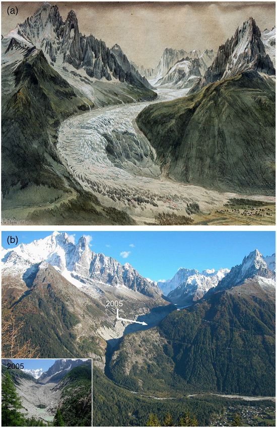
shows the location of the glacier front in 2005.H.J. Zumbühl et al. / Global and Planetary Change 60 (2008) 42–57 55 Fig. 10. (a) Samuel Birmann portrayed in 1823 the Mer de Glace 1823 from la Flégère (20.6 × 47.1 cm; pencil, pen, watercolor, bodycolor; cut-out). Kupferstichkabinett, Kunstmuseum Basel. Photograph by Heinz J. Zumbühl. (b) Recent view of the Mer de Glace. Photograph by Samuel U. Nussbaumer, 8.10.2005. Again, the arrow shows the location of the glacier front in 2005. different configurations of climate variables lead to a Length variations are shown to behave as a lagged glacier advance/retreat. The advance towards 1820 was process, with a glacier-specific memory of past climatic presumably driven by low summer temperatures and conditions. high autumn precipitation. The 1860–1880 retreat Finally, the present nonlinear neural network period was mainly determined by high temperatures. approach seems to be a powerful tool in a glaciological However, temperature seems to be the primary driver context. Because the limitations and chances of this of the mid 19th maximum extent and subsequent nonlinear technique are not fully explored, further retreat, precipitation plays a secondary role. We also investigations towards a “neuro-glaciology” should be conclude that the Lower Grindelwald Glacier shows a done, including different glaciers in different climate time-dependent, dynamic response to climatic change. regions.
56                                    H.J. Zumbühl et al. / Global and Planetary Change 60 (2008) 42–57

Acknowledgements                                                              (NSIDC)/World Data Center for Glaciology, University of Color-
                                                                              ado, Boulder, CO, CD-ROM.
                                                                          Kempf, C., 1994. Adolphe Braun et la photographie, 1812–1877.
   This study was supported by the Swiss National                             Editions Lucigraphie/Valblor, Illkirch, France.
Science Foundation, through its National Centre of                        Kirchhofer, W., Sevruk, B., 1992. Mittlere jährliche korrigierte
Competence in Research on Climate (NCCR Climate),                             Niederschlagshöhen 1951–1980. In: Weingartner, R., Spreafico,
project PALVAREX. The authors are grateful to J.                              M. (Eds.), Hydrologischer Atlas der Schweiz. Bundesamt für
                                                                              Landestopografie, Bern-Wabern.
Luterbacher and A. Pauling for providing multiproxy
                                                                          Luterbacher, J., Dietrich, D., Xoplaki, E., Grosjean, M., Wanner, H.,
reconstructions of temperature and precipitation.                             2004. European seasonal and annual temperature variability,
Thanks also go to C. Vincent and the LGGE                                     trends, and extremes since 1500. Science 303 (5663), 1499–1503.
(Laboratoire de Glaciologie et Géophysique de l’Envir-                    Maisch, M., Wipf, A., Denneler, B., Battaglia, J., Benz, C., 1999. Die
onnement, Saint-Martin-d'Hères cedex, France) for                             Gletscher der Schweizer Alpen. Gletscherhochstand 1850,
providing data from the Mer de Glace. We also wish                            Aktuelle Vergletscherung, Gletscherschwund-Szenarien. Vdf
                                                                              Hochschulverlag, ETH Zürich.
to thank R. Eggimann and D. Mihajlovic from                               Matthews, J.A., Briffa, K.R., 2005. The ‘Little Ice Age’: re-evaluation
Photogrammetrie Perrinjaquet AG, Gümligen, Switzer-                           of an evolving concept. Geografiska Annaler 87A (1), 17–36.
land, for their help in photogrammetric interpretation of                 Michaelsen, J., 1987. Cross-validation in statistical climate forecast
aerial photographs and the generation of digital eleva-                       models. Journal of Applied Meteorology 26 (11), 1589–1600.
tion models (DEMs).                                                       Mougin, P., 1912. Etudes glaciologiques. Savoie-Pyrénées, Tome III.
                                                                              Imprimerie Nationale, Paris.
                                                                          Nussbaumer, S.U., Zumbühl, H.J., Steiner, D., in press. Fluctuations of
References                                                                    the “Mer de Glace” (Mont Blanc area, France) AD 1500–2050: an
                                                                              interdisciplinary approach using new historical data and neural
Birmann, S., 1826. Souvenirs de la Vallée de Chamonix. Birmann et             network simulations. Zeitschrift für Gletscherkunde und
   fils, Basel.                                                               Glazialgeologie.
Chlumsky, M., Eskildsen, U., Marbot, B., 1999. Die Brüder Bisson.         Oerlemans, J., 2005. Extracting a climate signal from 169 glacier
   Aufstieg und Fall eines Fotografenunternehmens im 19. Jahrhun-             records. Science 308 (5722), 675–677.
   dert. Katalog zur gleichnamigen Ausstellung: Museum Folkwang,          Oerlemans, J., Reichert, B.K., 2000. Relating glacier mass balance to
   Essen, 07.02.–28.03.1999; Fotomuseum im Münchner Stadtmu-                  meteorological data by using a seasonal sensitivity characteristic.
   seum, 11.04.–30.05.1999; Bibliothèque nationale de France, Paris,          Journal of Glaciology 46 (152), 1–6.
   15.06.–15.08.1999. Verlag der Kunst, Amsterdam.                        Pauling, A., Luterbacher, J., Casty, C., Wanner, H., 2006. Five hundred
de Decker Heftler, S., 2002. Photographier le Mont Blanc. Les                 years of gridded high-resolution precipitation reconstructions over
   pionniers – Collection Sophie et Jérôme Seydoux. Editions                  Europe and the connection to large-scale circulation. Climate
   Guérin, Chamonix.                                                          Dynamics 26 (4), 387–405.
Grove, J.M., 2004. Little Ice Ages: Ancient and Modern, 2nd edition.      Reichert, B.K., Bengtsson, L., Oerlemans, J., 2001. Midlatitude
   Routledge, London.                                                         forcing mechanisms for glacier mass balance investigated using
Haeberli, W., Hoelzle, M., 1995. Application of inventory data for            general circulation models. Journal of Climate 14 (17),
   estimating characteristics of and regional climate-change effects on       3767–3784.
   mountain glaciers: a pilot study with the European Alps. Annals of     Rumelhart, D.E., Hinton, G.E., Williams, R.J., 1986. Learning internal
   Glaciology 21, 206–212.                                                    representations by error propagation. In: Rumelhart, D.E., McClel-
Haeberli, W., Zumbühl, H.J., 2003. Schwankungen der Alpengletscher            land, J.L. (Eds.), Parallel Distributed Processing: Explorations
   im Wandel von Klima und Perzeption. In: Jeanneret, F., Wastl-              in the Microstructure of Cognition. MIT Press, Cambridge, MA,
   Walter, D., Wiesmann, U., Schwyn, M. (Eds.), Welt der Alpen –              pp. 318–362.
   Gebirge der Welt, Ressourcen, Akteure, Perspektiven. Haupt,            Schmeits, M.J., Oerlemans, J., 1997. Simulation of the historical
   Bern, pp. 77–92.                                                           variations in length of Unterer Grindelwaldgletscher, Switzerland.
Holzhauser, H., Zumbühl, H.J., 1996. To the history of the Lower              Journal of Glaciology 43 (143), 152–164.
   Grindelwald Glacier during the last 2800 years – palaeosols,           Steiner, D., Walter, A., Zumbühl, H.J., 2005. The application of a non-
   fossil wood and historical pictorial records – new results.                linear back-propagation neural network to study the mass balance
   Zeitschrift für Geomorphologie, Neue Folge, Supplementband                 of Grosse Aletschgletscher, Switzerland. Journal of Glaciology 51
   104, 95–127.                                                               (173), 313–323.
Holzhauser, H., Zumbühl, H.J., 2003. Nacheiszeitliche Gletscher-          Steiner, D., Zumbühl, H.J., Bauder, A., in press. Two Alpine Glaciers
   schwankungen. In: Weingartner, R., Spreafico, M. (Eds.), Hydro-            over the Past Two Centuries: A Scientific View Based on Pictorial
   logischer Atlas der Schweiz. Special edition for the 54th                  Sources. In: Orlove, B., Wiegandt, E., Luckman, B. (Eds.),
   “Deutscher Geographentag” in Berne (revised). Bundesamt für                Darkening Peaks: Glacial Retreat, Science and Society. University
   Landestopografie, Bern-Wabern.                                             of California Press, Berkeley, CA.
Holzhauser, H., Magny, M., Zumbühl, H.J., 2005. Glacier and lake-         Stone, M., 1974. Cross-validation choice and the assessment of
   level variations in west-central Europe over the last 3500 years.          statistical predictions. Journal of the Royal Statistical Society. Series
   The Holocene 15 (6), 791–803.                                              B 36 (1), 111–147.
Imhof, M., 1998. Rock glaciers, Bernese Alps, western Switzerland.        Walter, A., Schönwiese, C.-D., 2002. Attribution and detection of
   In: International Permafrost Association, Data and Information             anthropogenic climate change using a backpropagation neural
   Working Group (Eds.), National Snow and Ice Data Center                    network. Meteorologische Zeitschrift 11 (5), 335–343.
H.J. Zumbühl et al. / Global and Planetary Change 60 (2008) 42–57 57 Walter, A., Schönwiese, C.-D., 2003. Nonlinear statistical attribution derts. Ein Beitrag zur Gletschergeschichte und Erforschung des and detection of anthropogenic climate change using simulated Alpenraumes. Denkschriften der Schweizerischen Naturforschenden annealing algorithm. Theoretical and Applied Climatology 76 Gesellschaft (SNG), Band 92. Birkhäuser, Basel/Boston/Stuttgart. (1–2), 1–12. Zumbühl, H.J., 1997. Die Hochgebirgszeichnungen von Samuel Wang, W., Jones, P., Partridge, D., 2000. Assessing the impact of input Birmann – ihre Bedeutung für die Gletscher– und Klimageschichte. features in a feedforward neural network. Neural Computing and Katalog zur Ausstellung “Peter und Samuel Birmann – Künstler, Applications 9 (2), 101–112. Sammler, Händler, Stifter” des Kunstmuseums Basel vom Wetter, W., 1987. Spät– und postglaziale Gletscherschwankungen im 27.09.1997–11.01.1998. Schwabe Verlag, Basel. Mont Blanc-Gebiet: Untere Vallée de Chamonix – Val Montjoie. Zumbühl, H.J., Holzhauser, H., 1988. Alpengletscher in der Kleinen Physische Geographie, Vol. 22. Geographisches Institut der Eiszeit. Sonderheft zum 125jährigen Jubiläum des SAC. Die Alpen Universität Zürich, Zürich. 64 (3), 129–322. Xoplaki, E., Luterbacher, J., Paeth, H., Dietrich, D., Steiner, N., Zumbühl, H.J., Messerli, B., Pfister, C., 1983. Die kleine Eiszeit: Grosjean, M., Wanner, H., 2005. European spring and autumn Gletschergeschichte im Spiegel der Kunst. Katalog zur Sonder- temperature variability and change of extremes over the last half ausstellung des Schweizerischen Alpinen Museums Bern und des millennium. Geophysical Research Letters 32 (15), L15713. Gletschergarten-Museums Luzern vom 09.06.–14.08.1983 Zumbühl, H.J., 1980. Die Schwankungen der Grindelwaldgletscher in (Luzern), 24.08.–16.10.1983 (Bern). den historischen Bild- und Schriftquellen des 12. bis 19. Jahrhun-
You can also read