2021 Line-Haul Locomotive Emission Inventory Air Quality Planning and Science Division Mobile Source Analysis Branch February 2021

2021 Line-Haul Locomotive Emission Inventory

 Air Quality Planning and Science Division
 Mobile Source Analysis Branch
 February 2021

 1

Contents
Executive Summary......................................................................................................................... 4
Inventory Inputs and Methodology ................................................................................................ 6
 Line-haul Population and Activity Data ..................................................................................................................6
 Tier Distribution of Locomotives in Source Data ....................................................................................................7
 Emission Factors .....................................................................................................................................................8
Forecasting Methodology ............................................................................................................... 8
 Transition Patterns between Tier Groups ..............................................................................................................9
 Baseline Growth Rate of Total MWhrs ................................................................................................................ 10
 MWhrs Forecasting Methodology ....................................................................................................................... 13
 Prediction of Major Turnover Timing .................................................................................................................. 15
 Tier Distribution Baseline (BAU Case) ................................................................................................................. 19
 Scaling South Coast to Statewide Emissions ....................................................................................................... 23
Emissions Results (BAU Case) ....................................................................................................... 24

Tables
Table 1. US EPA Line-haul Emission Factors for NOx and PM10 in g/bhp-hr .............................................................8
Table 2. Freight Movement-related Growth Rate Forecasts................................................................................... 11
Table 3. Predicted Major Turnover Timing (years).................................................................................................. 18
Table 4. The Conversion Factor Used for MWhrs Extrapolation ............................................................................. 23
Table 5. Line-haul Locomotive NOx and PM emissions (tpd) in South Coast (SC), San Joaquin Valley (SJV), and
California Statewide (CA)......................................................................................................................................... 25

Figures
Figure 1: Comparison of 2016 and 2020 Line-haul NOx Emissions Inventory in Tons Per Day (tpd) .........................5
Figure 2: NOx Emission Contribution by Sector in 2020 and 2035 ............................................................................5
Figure 3: Tier Distribution in Unit Population ............................................................................................................6
Figure 4: SC MWhrs Distribution for the Recent Nine Years ......................................................................................7
Figure 5: MWhrs Transition Between Tiers due to Remanufacturing ..................................................................... 10
Figure 6. Freight Movement-related Growth Rate Forecasts ................................................................................. 12
Figure 7: MWhrs of Line-haul Locomotive Forecasting Procedure ......................................................................... 13
Figure 8: Deficits of the Total MWhrs of the Tier Groups Compared to the Base MWhrs Growth ........................ 14
Figure 9: Total Service Life per Tier ......................................................................................................................... 16
Figure 10: Distribution of MWhrs per Unit and Average Reman Cycle (ARC) ......................................................... 16
Figure 11: Average Remanufacturing Cycle ............................................................................................................ 17
Figure 12: Predicted Average Service Time until Major Turnover .......................................................................... 18
Figure 13: MWhrs Distribution based on the Given MWhrs Growth Rates for the Past 9 Years ........................... 19

 2

Figure 14: MWhrs Distribution based on Tier Transition Patterns (MWhrs Flows) ................................................ 20
Figure 15: MWhrs Distribution Considering Anticipated Retirement Patterns ...................................................... 20
Figure 16: MWhrs Share (%) of the Tier Groups ..................................................................................................... 21
Figure 17: Tier Allocation of Replacement in Business-As-Usual Scenario ............................................................. 22
Figure 18: BAU Scenario Tier Distribution ............................................................................................................... 22
Figure 19: Allocations of SC Line-haul and Switcher MWhrs over Statewide MWhrs ............................................ 23
Figure 20: Projected South Coast NOx Emissions (tpd) by Tier vs. 2016 SC SIP Inventory ..................................... 24
Figure 21: Statewide NOx Projections by Tier and 2016 SIP NOx Values ................................................................ 24

 3

Executive Summary
Locomotives and rail systems are an important part of California's freight and passenger movement
network and are significant contributors to harmful diesel emissions in California. This document
summarizes the methodology utilized by the California Air Resources Board (CARB) to estimate
emissions from Class I line-haul locomotives which include locomotives that provide interstate freight
transportation for containers, liquid material, or bulk material in California. The Surface Transportation
Board defines Class I line-hauls as operations that gross over $450 million per year1,2. There are six
Class I line-haul operations in the United States, with two operating in California: Union Pacific (UP)
Railroad and BNSF Railway. Additional locomotive categories not included in this inventory are Class II
and III line-hauls, passenger locomotives, and switching locomotives that are used within railyards.
This updated emissions inventory is developed using line-haul activity and population supplied by both
UP and BNSF railroads. The previous emissions inventory model was developed in 2011 based on
2007/2008 data and was later updated in 2016. Considering that previous inventories were developed
prior to the penetration of Tier 4 engines, they were not able to predict how locomotive companies
would adopt Tier 4 engines or respond to the new engine standards. Both releases predicted a
relatively fast penetration of Tier 4 locomotives in the fleet - at a rate of up to 7 percent per year after
2015. In retrospect, the predicted penetration rate turned out to be very optimistic and has not
materialized. According to the most recent data, Tier 4 locomotive engine penetration rates sit at
under 1 percent per year on average because the railroads have been purchasing fewer than expected
Tier 4 units for the past few years, instead choosing to operate remanufactured Tier 1+ and Tier 2+
units.
Figure 1 shows the updated emission projections and the previous emission inventory (shown in the
dotted red line) that was used for the 2016 South Coast State Implementation Plan. As shown, due to
the lack of Tier 4 locomotive engine penetration in the fleet, the updated Class I line-haul inventory
shows increased emissions for both nitrogen oxides (NOx) and particulate matter (PM) compared to
previous inventories. Barring a change in this behavior, either internal or due to regulatory or incentive
actions, locomotive emissions are projected to continue to increase through 2032. This trend will make
locomotives an increasingly important mobile source sector for future air quality planning and policy
development as emissions from other sources such as diesel trucks and construction equipment are
decreasing significantly over the same period.

1
 Freight Facts and Figures 2017, US Department of Transportation and Bureau of Transportation Statistics, available at:
https://www.bts.gov/sites/bts.dot.gov/files/docs/FFF_2017.pdf
2
 Freight Railroads Background, Office of Rail Policy and Development, Federal Railroad Administration, April 2015, available at:
https://railroads.dot.gov/sites/fra.dot.gov/files/fra_net/14497/Freight%20Railroads%20Background%20April_2015.pdf

 4

Figure 1: Comparison of 2016 and 2020 Line-haul NOx Emissions Inventory in Tons Per Day (tpd3)

 15.0

 12.0
 NOx emissions (tpd)

 9.0

 6.0

 3.0

 0.0
 2020 2022 2024 2026 2028 2030 2032 2034 2036 2038 2040 2042 2044 2046 2048 2050
 PRE-TIER 0 TIER 0/0+ TIER 1/1+ TIER 2/2+
 TIER 3 TIER 4 2020 SC BAU Inventory 2016 SC SIP Inventory

Figure 2 presents the relative emissions contribution of line-hauls compared to other mobile sources,
demonstrating the increasing importance of line-haul emissions over time. Separately from the direct
contribution, it is notable that locomotives in freight movement offer substantially lower energy
footprints than other freight transportation modes, such as road/trucks, pipeline, and waterways4 per
gross ton-mile of cargo moved.
 Figure 2: NOx Emission Contribution by Sector in 2020 and 20355

 Light-duty 2020 Light- and Medium- Light-duty 2035
 vehicles, 5.5% Light- and Medium-
 duty trucks, 8.8% vehicles, 3.6%
 duty trucks, 3.3%
 Farm
 equipment, 8.2% Farm equipment,
 4.9%
 Offroad Offroad
 equipment, Heavy duty equipment, 14.0% Heavy duty
 14.1% trucks, 39.4% trucks, 38.4%

 OGVs & OGVs & others,
 others, 7.4% 10.8%
 Buses, Buses,
 Aircraft, 1.7% Aircraft, 1.1%
 Locomotives, 8.2% 5.4% Locomotives, 13.1% 9.5%

3
 Short tons per day
4
 Rail travel is cleaner than driving or flying, but will Americans buy in?, Andreas Hoffrichter, 2015, available at:
https://theconversation.com/rail-travel-is-cleaner-than-driving-or-flying-but-will-americans-buy-in-112128
5
 These charts do not account for recently adopted regulations such as HD Omnibus and Advanced Clean Trucks

 5

Inventory Inputs and Methodology
Line-haul Population and Activity Data
In 1998, CARB and CA railroads (RRs) agreed to a memorandum of understanding (MOU) for
accelerated adoption of cleaner locomotives in the South Coast region. In conjunction with the MOU
and the locomotive engine emission standards, the RRs agreed to ensure the South Coast locomotive
fleet met a Tier 2 engine average by 2010. To verify Fleet Average Targets in the MOU are being met,
UP and BNSF must track and report locomotive usage in the South Coast Nonattainment Area by
recording megawatts-hours (MWhrs) and fuel consumption.
The 2020 updated line-haul model is developed primarily on the 1998 MOU data for locomotives
operating in South Coast Air Basin (SCAB) supplied by BNSF and UP from 2010 to 2018. The 2018 data
serves as the base year for population and activity, and the forecasting model is based on the
remanufacturing behavior and MWhrs transition patterns between Tier groups observed between
2015 to 2018. This report discusses the methodology employed by CARB staff to determine future
locomotive activity, Tier distribution, and resulting emissions.
Tier distribution and turnover patterns shown in the SCAB were used for determining Tier and turnover
patterns for the remainder of the state. The SCAB data was used because the data set is significantly
more robust, has more years represented, and has a higher temporal resolution. The activity, in
MWhrs, for the remainder of the state, was based on data supplied by UP and BNSF. An overall Tier
distribution for the remainder of the state was also supplied at a lower resolution; however, as shown
in Figure 3, The statewide Tier distribution was not significantly different in 2018 than the one in South
Coast. Hence the more robust South Coast data set was used to determine the activity and Tier
transition patterns across the state.
 Figure 3: Tier Distribution in Unit Population

 6

Remanufacturing a locomotive generally means replacing older, worn-out engine components with
either freshly manufactured power assemblies or refurbished assemblies. Remanufacturing includes
engine replacements, upgrades, and conversion of engine emissions control systems; therefore, a
locomotive's engine Tier can be changed from one Tier to another after the remanufacture. The
emission standard of the remanufactured units depends on the remanufacture kit. These units are
identified as different emission standards, such as Tier 1r, or 1+, 2r or 2+, etc. The following sections
will cover the existing data, the observed pattern of transitions between Tiers, the projected overall
growth, and lastly, how these inputs combine to form the forecast.

Tier Distribution of Locomotives in Source Data
Figure 4 shows the megawatts-hours (MWhrs) distribution of locomotive Tier groups operated in the
South Coast Air Basin from 2010 to 2018. For the past nine years, the majority of Tier 1 and 2 units
have been replaced by Tier 1+ and Tier 2+, respectively. MWhrs of Tier 4 shows a slow adoption rate
from 2016 through 2018, while the MWhrs of Tier 3 have remained steady for the past three years.
Tier 1+ notably became the largest contributor to MWhrs in 2018. Tier 4 locomotive purchases have
been steadily decreasing since Tier 4 standards went into effect in 2015, with no 2019 Tier 4
locomotive purchases as of May 31, 2019, which is again indicating the low adoption of Tier 4
locomotive by railyards.
 Figure 4: SC MWhrs Distribution for the Recent Nine Years

 500
 Megawatts-hours (thousands)

 400

 300

 200

 100

 0
 2010 2011 2012 2013 2014 2015 2016 2017 2018

 PRE-TIER 0 TIER 0 TIER 0+ TIER 1 TIER 1+ TIER 2 TIER 2+ TIER 3 TIER 4

 7

Emission Factors
The updated emissions inventory model uses the line haul emission factors, by Tier, published by U.S.
Environmental Protection Agency (US EPA)6 as shown in Table 1. As illustrated in this table, Tier 4
engines offer significantly lower NOx and diesel PM2.5 emission rates compared to older Tiers. This
shows the importance of Tier 4 engine adoption in reducing NOx emissions from the rail sector in
California.
 Table 1. US EPA Line-haul Emission Factors for NOx and PM10 in g/bhp-hr
 Tier PM10 NOx
 Pre-Tier 0 0.320 13
 Tier 0 0.320 8.6
 Tier 0+ 0.200 7.2
 Tier 1 0.320 6.7
 Tier 1+ 0.200 6.7
 Tier 2 0.180 4.95
 Tier 2+ 0.080 4.95
 Tier 3 0.080 4.95
 Tier 4 0.015 1.0

Forecasting Methodology
Looking at the rail data for the past nine years, the Tier distribution shows different activity levels and
turnover patterns in each year. The turnover pattern will determine which engine Tiers are seeing
increased activity, which ones are phasing out (also known as diminishing Tiers), which ones are being
remanufactured, and what Tier are they being manufactured to. In addition, the available data covers
only the South Coast Air Basin, and each railroad can assign any of their units to California operations
from outside the state. Considering the Tier pattern over the past nine years, CARB inventory staff
recognized that a conventional survival curve - or demographic data-based approaches for predicting
locomotive turnover rates would not be the most appropriate modeling technique for this category.
Conventional methods generally rely on a captive group of equipment that is retired and replaced on a
predictable schedule, and engines are not remanufactured to different Tiers in a complex or shifting
pattern.
Furthermore, conventional forecasting methods are limited to reflect work intensity per locomotive
unit, while in reality, the workload per unit can, and does, change over time. A heavy heavy-duty truck
is defined by the Federal Highway Administration (FHWA) as weighing 33,001 pounds and greater,
while a modern railcar's gross capacity is around 286,000 pounds. Locomotives can stretch from 10,000
to 15,000 feet in length by pulling as many as one hundred railcars. As a result, the total weight pulled
by Class I locomotives can vary significantly depending on the length of the train and the type of

6
 Emission Factors for Locomotives, United States EPA, December 1997, available at:
https://nepis.epa.gov/Exe/ZyPURL.cgi?Dockey=P1001Z8C.TXT

 8

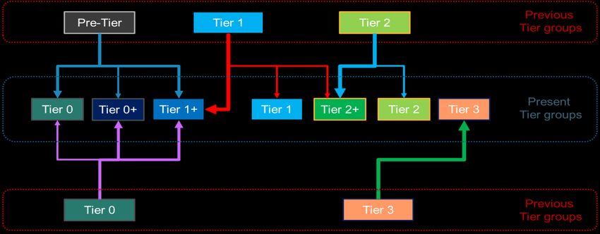
commodity being transported. Based on the aforementioned reasons, this inventory uses MWhrs
(activity) as the basis for the inventory instead of the population of locomotives.
Traditional locomotive inventory methods generally focus on equipment turnover and neglect the
impact of remanufacturing. Therefore, this new CARB inventory uses a replacement and
remanufacture behavior-based modeling approach – essentially focusing on the shift between Tier
groups in addition to equipment turnover cycles. This new inventory bases the Tier transition forecast
on information for locomotives visiting the South Coast Air Basin because this is the most robust
dataset provided to CARB by the rail companies. Assuming rail companies provide information at
similar levels of detail for other parts of the state, CARB can update the inventory accordingly.
The basic model assumptions assumed for this inventory update are:
 1. MWhrs from the South Coast MOU7 data are used to calculate fuel use and emissions
 (accounting for engine Tier) for each locomotive. This is the foundation for forecasting MWhrs
 and emissions for future years.
 2. South Coast Air Basin line-haul operations are representative of statewide line-haul operations.
 This means that the model assumed other air basins have similar remanufacture and
 replacement behavior. The model presumes SCAB's pattern of diminishing MWhrs is identical
 to statewide fleet turnover patterns, which is supported by the similarity of Tier distributions
 between SCAB and the rest of California, as shown in Error! Reference source not found..
 3. Railroads (RRs) will remanufacture the locomotive units in CA operation in a similar pattern, as
 demonstrated over the past decade. As a result, the SC Tier distribution will change over time,
 but the MWhrs transition patterns between Tier groups will remain consistent in future years.
 The observed Tier transition patterns were used to predict incremental MWhrs per year and
 Tier distributions in the coming years.
 a. The suggested model presumes that total MWhrs of old Tier groups, such as Pre-Tier 0,
 T1, T1+, etc., will start to diminish after the major turnover timing that the majority of
 each Tier group is retired or remanufactured (this is described in detail later in the
 document). This relies on the assumption that turnover patterns of the statewide fleet
 are similar to those of the nationwide fleet.
 b. 1998 MOU data obtained from 2010 to 2018 reasonably presents the movement of
 MWhrs between Tier groups, and this inventory assumes that the transition patterns
 will continue in the next decades.

Transition Patterns between Tier Groups
The Tier distribution of locomotives in the South Coast from 2010 to 2018 is the basis for forecasting
future Tier distributions. Figure 5 shows the observed MWhrs flows between Tier groups during this

7
 CARB Rail Emission Reduction Agreements, available at: https://ww2.arb.ca.gov/resources/documents/rail-emission-
reduction-agreements

 9

period. For example, 1,218 Pre-Tier locomotives were remanufactured to a Tier 0 emission standard.
The most significant observed patterns of the MWhrs remanufactures are:
 • From Pre-Tier 0 to Tier 0 and Tier 1+,
 • Tier 0 to Tier 0+,
 • Tier 1 to Tier 1+,
 • Tier 2 to Tier 2+.
 Figure 5: MWhrs Transition Between Tiers due to Remanufacturing

Baseline Growth Rate of Total MWhrs
The base MWhrs growth was predicted using the Freight Analysis Framework (FAF) version 4.5.1 data8,
as well as the historic railroad growth rates. FAF is produced through a partnership between the
Bureau of Transportation Statistics (BTS) and Federal Highway Administration (FHWA). It collects data
from a variety of sources to create a comprehensive picture of freight movement among states and
major metropolitan areas by all modes of transportation. The main sources of information are the
Commodity Flow Survey (CFS) and international trade data from the Census Bureau. FAF provides
forecasts as estimates for tonnage and value by regions of origin and destination, commodity type, and
mode. The FAF forecast is used in forecasts by California Statewide Freight Forecasting Model (CSFFM)
developed by CalTrans, as well as the Bay Area Metropolitan Transportation Commission for San
Francisco Bay Area Goods Movement Plan9. Equation 1 shows how projections from FAF as well as the
historic railroad growth rates were used to determine the future growth rates for rail activity in
California. On the left of the equation, the historical FAF forecast rate (i.e., 2.249 percent growth per
year) is compared to the observed growth rate of MWhrs in the railroad data (i.e., 2.777 percent per
year). From this relationship, we can see that the railroad MWhrs experienced a higher growth rate

8
 Freight Analysis Framework Version 4 available at: https://faf.ornl.gov/fafweb/
9
 Metropolitan Transportation Commission, San Francisco Bay Area Goods Movement Plan, February 2016,
https://mtc.ca.gov/sites/default/files/RGM_Full_Plan.pdf

 10

than is forecasted by FAF. Applying this relationship to the current forecast for California rail in FAF 4.5
(1.773 percent per year), expected growth from the railroads will be 2.19 percent per year.
 15, ℎ ℎ ( ) 45, ℎ ℎ ( )
 =
 ℎ ℎ ℎ ℎ ℎ 

 2.249% 1.773%
 =
 2.777% ℎ ℎ = 2.1898%
 Table 2. Freight Movement-related Growth Rate Forecasts
 Average
Data sources Time frame
 Growth
Total Distillate Sales/Deliveries to Railroad Consumers (Thousand Gallons) 10 2013–2018 1.82%
CA State Rail Plan: Compound annual growth rates for carload service11 2013–2040 1.70%
CA State Rail Plan: Compound annual growth rates for intermodal service11 2013–2040 2.90%
 12
ATA 2012 Rail Volume Forecast: Rail Carload & Intermodal Freight 2012–2023 1.42%
2019 The Budget and Economic Outlook: GDP (Billions of dollars) 13 2013–2018 4.70%
2020 SCAG SoCal Connect – Goods Movement Plan14 2020-2045 2.8%
Rail growth used for SCAG Regional Transportation Planning15 2010–2018 3.30%
Class I Rail Freight Fuel Consumption and Travel (million gallons)16 2010–2018 1.51%
 16
Seasonally adjusted Rail Freight Intermodal Traffic (BTS & AAR) 2010–2018 3.17%
Port of Long beach container counts (TEUs)17 2010–2018 2.20%
Port of LA container counts (TEUs)18 2010–2018 2.00%

In addition to reviewing FAF data, the data source is compared against a number of sources to
determine if the FAF forecast was reasonable. Table 2 and Figure 6 present the calculated growth rates
from multiple data resources and confirms the value from FAF is within a reasonable range of other
data sources. It is notable that the growth used in this emissions inventory is significantly below those

10
 U.S. Energy Information Administration, Sales of Distillate Fuel Oil by End Use,
https://www.eia.gov/dnav/pet/pet_cons_821dst_dcu_nus_a.htm
11
 California State Rail Plan, https://dot.ca.gov/programs/rail-and-mass-transportation/california-state-rail-plan
12
 http://www.azttca.org/pdf/ATA-Freight-Forecast.pdf
13
 The Budget and Economic Outlook: 2019 to 2029 of Congressional budget office (CBO),
https://www.cbo.gov/system/files/2019-03/54918-Outlook-3.pdf
14
 2020 Connect SoCal Goods Movement Plan, Adopted on September 3, 2020, https://scag.ca.gov/sites/main/files/file-
attachments/0903fconnectsocal_goods-movement.pdf?1606001690
15
 2012-2035 Regional Transportation Plan (RTP) of the Southern California Association of Governments,
http://rtpscs.scag.ca.gov/Pages/2012-2035-RTP-SCS.aspx
16
 Bureau of transportation statistics: Class I Rail Freight Fuel Consumption and Travel, https://www.bts.gov/content/class-i-
rail-freight-fuel-consumption-and-travel
17
 Port of Long Beach latest statistics, https://www.polb.com/business/port-statistics/#latest-statistics
18
 Port of LA container statistics, https://www.portoflosangeles.org/business/statistics/container-statistics

 11

suggested by the state rail plan, the Southern California Association of Governments (SCAG) 2020
regional transportation plan (2020 RTP)19, or the Bureau of Transportation Statistics and American
Association of Railroads growth totals over the last decade, but instead is closer to the historical
growth rates of fuel used by the railroads. For example, according to SCAG's Goods Movement Plan,
between 2020 and 2045, freight train volumes are expected to more than double, and intermodal lift
volumes are expected to grow by more than 140 percent. That is almost an average of 2.8% year over
year growth for freight train volumes between 2020–2045 which is higher than the 2.19 percent
growth assumed for this emissions inventory update.
There are some indications that efficiency may change from the current forecast, as the RRs are
attempting to make a transition to precision scheduled railroading (PSR), which is expected to enhance
the system efficiency. CARB will continue to monitor rail data to determine if rail efficiencies need to
be reflected in future inventories.
 Figure 6. Freight Movement-related Growth Rate Forecasts

 5%
 Average growth rate (%)

 4%

 3%

 2%

 1%

 0%
 2010 2012 2014 2016 2018 2020 2022 2024 2026 2028 2030 2032 2034 2036 2038 2040 2042 2044
 Total Distillate Sales/Deliveries to Railroad Consumers (Thousand Gallons)
 CA State Rail Plan: Compound annual growth rates for carload service
 CA State Rail Plan: Compound annual growth rates for intermodal service
 ATA 2012 Rail Volume Forecast: Rail Carload & Intermodal Freight
 2019 The Budget and Economic Outlook: GDP (Billions of dollars)
 2020 SCAG Socal Connect – Goods Movement Plan
 Rail growth used for SCAG Regional Transportation Planning
 Class I Rail Freight Fuel Consumption and Travel (million gallons)
 Seasonally-adjusted Rail Freight Intermodal Traffic (BTS & AAR)
 Port of Long beach container counts (TEUs)
 Port of LA container counts (TEUs)[10]
 Line-haul locomotive activity growth rate

19
 2020 Connect SoCal Goods Movement Plan, Adopted on September 3, 2020, https://scag.ca.gov/sites/main/files/file-
attachments/0903fconnectsocal_goods-movement.pdf?1606001690

 12

MWhrs Forecasting Methodology
As described earlier, the forecasting model is based on the observed transition between Tiers, as well
as the application of growth to the total MWhrs. The resulting MWhrs distribution for future years will
show that some Tier groups will be phased out, while others will grow and take over the diminishing
MWhrs of the Tier groups that are phasing out. The forecasting process is presented in Figure 7.
 Figure 7: MWhrs of Line-haul Locomotive Forecasting Procedure

The updated model organizes the nine Tier groups into two bins that are expected to either grow or
diminish based on observed trends. Increasing Tier groups (ITGs), including Tier 0+, 1+, 2+, 3, and 4,
have increased in the past decade and are projected to increase in future years. The other Tiers are
arranged into Decreasing Tier groups (DTGs), which have negative growth rates based on the 2010 to
2018 period. The MWhrs increase for ITGs is directly correlated to the MWhrs decreases of DTGs, such
as Pre-Tier, Tier 0, Tier 1, and Tier 2. Incremental MWhrs of ITGs are calculated based on the process
described below.
 1. Future MWhrs of Tier 0+, 1+, and 2+ are equal to the sum of the previous year's MWhrs and
 MWhrs transferred from Decreasing Tier Groups.

 13

a. For example, as shown in Figure 5, the sources of incoming MWhrs for Tier 0+ are Pre-
 Tier and Tier 0. The increase of MWhrs of Tier 0+ relies on the decreasing MWhrs of Pre-
 Tier and Tier 0 and then the percent of those Tier groups that are remanufactured to
 Tier 0+. Incremental MWhrs growth of Tier 0+ in a year (t) will be the same as the sum
 of decreased MWhrs of Decreasing Tier Groups in the previous year (t-1), in this case,
 10% and 39% of reduced MWhrs of Pre-Tier 0 and Tier 0, respectively.
 2. Pre-Tier, Tier 0, Tier 1, and Tier 2 will be phased out at their (negative) growth rate observed
 from the South Coast data.
 a. MWhrs of the following Tier groups group decrease at a negative growth rate per year:
 i. Pre-Tier 0: 14.0%
 ii. Tier 0: 4.8%
 iii. Tier 1: 26.6%
 iv. Tier 2: 14.1%
 b. The negative growth rate of Tier 0 is relatively low compared to the other groups, and as
 a result, Tier 0 would survive until 2040 at that rate. However, it is not likely that Tier 0
 would phase out more slowly than (more recently manufactured) Tier 1 and Tier 2;
 therefore, the inventory assumes that Tier 0 would start being turned over at a rate
 similar to Tier 1 locomotives in 2025 and later years.
 3. For Tier 3 and 4, this model uses the baseline growth rate, 2.19%. The growth rates obtained
 from the MOU data are varied and inconsistent, and there was no Tier 3 or Tier 4 adoption for
 the most recent years. Therefore, this inventory maintains a conservative approach to estimate
 future MWhrs of Tier 3 and 4.
In addition, the total MWhrs of all locomotive activity increases at the growth rate described in the
previous section. This creates a gap or deficit between expected MWhrs after the retirement and the
initial forecast. In Figure 8, the black line indicates baseline MWhrs growth, and the diagonally striped
area is representing the MWhrs deficit.
 Figure 8: Deficits of the Total MWhrs of the Tier Groups Compared to the Base MWhrs Growth
 1,000
 MWhrs needed for forecasted
 Decrease due to
 freight movement
 retirement, based on
 Megawatts-hours (thousand)

 800
 major-turning timing
In addition to the BAU scenario,
 described below
staff 600
 considered three additional approaches
 MWhrs to the MWhrs
deficit. In an optimistic scenario, the majority of MWhrs deficit can be
allocated to the newest Tier groups, such as Tier 3 and 4. However, discussionsDeficits
 with industry suggested
that there 400
 would be few purchases of locomotives over the next decade, making this scenario
unrealistic. Therefore, based on their initial contribution, Tier 1+, 2+, and 4 each takes 30% of the total
MWhrs deficits, while 10% goes to Tier 3. For the most optimistic scenario, 85% goes to Tier 4, and the
 200
rest is equally divided and distributed to the other remaining Tiers.

 0
 2010 2015 2020 2025 2030 2035 2040 2045 2050

 14

Prediction of Major Turnover Timing
Locomotive units are typically scrapped, parked, converted to switchers, or replaced by new ones after
a certain lifespan. According to the regulatory impact analysis report from USEPA, locomotives can run
over 40+ years20. Old units will eventually be retired and generally replaced by newer and cleaner
units. As a result, total locomotive emissions will be reduced as railroads adopt a greater fraction of
cleaner Tier units. Therefore, it is important to know the major turnover timing in which most
retirements occur (referred to in other cases as total service life, the average time to retirement,
average lifespan, etc.). The retirement year of each Tier can be anticipated by using the age
distribution and remaining operating time of the current line-haul fleet.
The most recent data submittals provided to CARB by the RRs show that locomotives' average service
life in the South Coast Air Basin operations is approximately 25 years which is different from U.S.
EPA's20. The age distribution of the locomotives shows a significant drop in population and activity at
25 years of age. CARB staff discovered that 84% of 22 ~ 24-year-old SC locomotives disappeared after
reaching 25 ~ 27 years. Twenty-five years of the total service life assumption was used to only predict
the major fleet turnover schedule upcoming in the next decade. This is because the future Tier mix in
CA operations could change over time as railroads introduce more advanced and cleaner locomotive
units. Since Tier 4 was officially introduced in 2015, railroads are still actively operating more Tier 1+
and Tier 2+ locomotives rather than adopting Tier 3 and Tier 4 locomotives. If railroads continue to run
them in the next decade, the average total service life of these locomotives in 2030 would be longer
than 25 years.
Assuming that railroads maintain the locomotive retirement patterns observed in recent years, the
inventory calculates the operating time remained for each Tier by subtracting the average age per Tier
from the average total service life. Figure 9 shows that the total service life consists of average age and
the remained operating time. As shown in the figure, recently remanned (remanufactured) Tier groups,
such as Tier 1+ and 2+, are likely to have longer periods of operating time remaining. The remaining
operating time over total service life was used to estimate the possible number of remanufacturing
cycles per Tier. Tier 0+ and Tier 1 groups show 18 years of average service life which is shorter than the
observed fleet average. CARB staff presumed that this is because the majority of the two Tier groups
were remanufactured to other Tiers before they reach their total service life. The inventory uses
calendar year (CY) 2016 as the base year to calculate the average age of the locomotive fleet. Tier 4
was officially introduced into CA operations in 2015; therefore, CY2016 is the first year that all Tier
groups were operated at the same time, and Tier 4 units turned to 1-year-old in that CY.

20
 Regulatory Impact Analysis: Control of Emissions of Air Pollution from Locomotive Engines and Marine Compression
Ignition Engines Less than 30 Liters Per Cylinder, https://nepis.epa.gov/Exe/ZyPURL.cgi?Dockey=P10024CN.txt

 15

Figure 9: Total Service Life per Tier

 Tier 2+ 1 24
 Tier 2 3 22
 Tier 1+ 2 23
 Tier 1 7 11
 Tier 0+ 5 13
 Tier 0 9 16
 Pre-Tier 0 9 16

 0 2 4 6 8 10 12 14 16 18 20 22 24 26 28

 Average Age since the last reman in 2016 Operating time remaining for the entire life in 2016

Remanufacturing behavior also affects turnover patterns. Using the South Coast locomotive visit
database, the inventory calculates the average remanufacturing cycle (ARC), which is the number of
years between each major overhaul of a locomotive engine. Unlike other mobile sources, railroads can
remanufacture locomotives units almost indefinitely. The model uses data from 2015 to 2018
submittals to determine the average time between remanufacturing to predict future remanufacturing
cycles.
For example, if model year (MY) 2010 locomotives in CA operations have a remanufacture cycle of 10
years, the engine will be remanufactured in 2020 for the first time. Then, every ten years thereafter,
assuming a functional limit of two remanufacturing cycles, the locomotive would be remanufactured in
2030 for a second time and then would likely be retired or removed from line-haul service in 2040. The
predicted remanufacturing and retiring years could be slightly changed depending on the work
intensity (MWhrs per unit) of individual units. If a line-haul locomotive operates more than average,
the unit will be remanned earlier than the other units started at the same time.
 Figure 10: Distribution of MWhrs per Unit and Average Reman Cycle (ARC)

 16

Average reman cycles (ARCs) vary by the annual activity of each Tier group. Tier groups with higher
MWhrs per unit have a shorter reman cycle due to longer annual operating hours. Figure 10 supports
this inverse relationship and indicates that the ARCs should be normalized by MWhrs per unit. Thus,
the inventory adjusts ARC based on the difference between the average MWhrs per unit and the Tier
groups' MWhrs per unit. Effectively, this means units with higher use are remanufactured more often,
as remanufactures are based on hours of use, not calendar years.
The remaining useful life is defined as the operating time remaining for a locomotive group and is
calculated by subtracting the average age (as also shown in 9) from the average reman cycle (ARC) for
each Tier group. Figure 11 shows the operating time from the last remanufacture, as well as the
forecasted remaining time before the next remanufacture based on the Tier-based ARC. Note that the
average reman cycle is equal to the average time between remanufactures, with an additional year for
the remanufacturing process to account for the time that the locomotive would be parked to complete
the process.
 Figure 11: Average Remanufacturing Cycle

 Tier 2+ 1 5
 Tier 2 3 3
 Tier 1+ 2 4
 Tier 1 7 3
 Tier 0+ 5 4
 Tier 0 9 2
 Pre-Tier 0 9 2

 0 1 2 3 4 5 6 7 8 9 10 11 12

 Average Age since the last reman in 2016 Operating time remaining for the current life in 2016

From base year 2016, locomotives are expected to operate for the period including the remaining life
before the following remanufacture and any remaining future service life based on the number of
remanufactures possible. The length of this future service life depends on the age of locomotives and
the remaining number of remanufactures. In other words, each Tier will have a different length of
future service life depending on the potential number of remanufactures that they can undergo. The
inventory determines how many times each Tier can be remanufactured in future years by considering
the age distribution of the Tier groups. The average ages of Tier 1+ / Tier 2 / Tier 2+ groups are lower
than the older Tiers and these Tier groups demonstrate the ability to have two remanufactures before
retirement. The older Tiers have approximately one remaining remanufacture prior to retirement due
to their older average age and resulting shorter remaining life.
Figure 12 presents how long the locomotives will continue to operate on average based on the
predicted major turnover timing. For Tier 3 and 4 locomotives, the inventory assumes that a major
turnover will occur 25 years after a locomotive is first introduced into service.

 17

Figure 12: Predicted Average Service Time until Major Turnover

 Tier 2+ 1 12
 Tier 2 3 12
 Tier 1+ 2 12
 Tier 1 7 10
 Tier 0+ 5 9
 Tier 0 9 11
 Pre-Tier 0 9 11

 0 2 4 6 8 10 12 14 16 18 20 22

 Average Age since the last reman in 2016 Future reman period

Table 3 shows the predicted major turnover timing with the related parameters also shown in Figures 9
and 11. Note that the numbers provided in this table present the year that the bulk portion of each
Tier is predicted to retire, while the phase-out starts several years earlier as the age distribution of
each Tier is generally a normal distribution. Figure 9 shows that CARB staff calculated the remaining
operating time for a given total service life by subtracting the average age (Column B) from the
Average retirement age (Column D, total service life). Figure 11 shows the sum of columns (B) and (C) is
equal to column (A) which is the average reman cycle. Column (F) of Major turnover timing is the sum
of 2016 (base year) and the predicted average service time of Figure 12.
 Table 3. Predicted Major Turnover Timing (years)
 Average age
 Remaining Average Operating time Major
 Activity- since the last
 useful life in retirement remaining for the total Turnover
 Tier Adjusted ARC reman in
 2016 age service life in 2016 Timing
 (A) 2016
 (C=A-B) (D) (E=D-B) (F)
 (B)
 Pre-Tier 11 9 2 25 16 2029
 Tier 0 11 9 2 25 16 2029
 Tier 0+ 9 5 4 18 13 2029
 Tier 1 10 7 3 18 11 2029
 Tier 1+ 6 2 4 25 23 2032
 Tier 2 6 3 3 25 22 2031
 Tier 2+ 6 1 5 25 24 2033
 Tier 3 - - - - - 2035
 Tier 4 - - - - - 2039

 18

Tier Distribution Baseline (BAU Case)
South Coast activity data shows that railroads (RRs) are likely to use older Tier locomotives than newer
Tier locomotives in recent years. For instance, total MWhrs of Tier 1+ has been increasing by 43.4
percent for the past nine years and became the largest contributing Tier group in 2017. Tier 2
accounted for 64 percent of the total MWhrs of the Tier groups in 2010, with the activity in MWhrs
gradually migrating to Tier 2+. Until 2014, Tier 2 was the largest contributor to MWhrs among the Tier
groups, however beginning in 2015, Tier 1+ became the largest single contributor. The Tier distribution
of the 2018 South Coast MOU data shows that 30.3 percent of total units operated in the South Coast
were Tier 1+. New Tier 3 units are no longer available for purchase, and the railroads have not
purchased any new Tier 4 units for the last two years in California. The BAU scenario reflects these
fleet turnover trends where the railroads operate Tier 1+ and Tier 2+ units more than the newer units.
Figures 13 and 14 present intermediate steps in the modeling process. Figure 13 shows the MWhrs
projections solely based on the growth rates obtained from MOU data without considering the lifespan
of locomotives or retirement. The Tier distribution presented in Figure 13 is an initial step only but is
not used as a final Tier distribution because it neglects the life cycle of locomotives and could
overestimate emissions. Figure 14 shows the MWhrs distributions adjusted by the Tier Transition
Patterns (TTP) discussed in the previous section called Transition Patterns between Tier Groups. The
MWhrs shifts in the Tier transition observed in the data forces some Tier groups to continue to
decrease while shifting their workload to the observed increasing Tier groups. This is a basic framework
for all scenarios considered in the forecasting process, and each analysis scenario will result in different
Tier distributions based on the given conditions, such as ARCs and MWhrs deficit allocations.
 Figure 13: MWhrs Distribution based on the Given MWhrs Growth Rates for the Past 9 Years

 1500 PRE-TIER 0 TIER 0 TIER 0+
 TIER 1 TIER 1+ TIER 2
 Megawatts-hours (thousands)

 TIER 2+ TIER 3 TIER 4
 Base MWhrs growth
 1000

 500

 0
 2010 2015 2020 2025 2030 2035 2040 2045 2050

The BAU scenario assumes no In-Use Locomotive Useful Life Limit in the CA operations; however, the
MWhrs of the Tier groups would naturally start to diminish in 2029, and the resulting MWhrs
distribution will be as shown in Figure 15.

 19

Figure 14: MWhrs Distribution based on Tier Transition Patterns (MWhrs Flows)

 1500 PRE-TIER 0 TIER 0 TIER 0+
 TIER 1 TIER 1+ TIER 2
 Megawatts-hours (thousands)

 TIER 2+ TIER 3 TIER 4
 Base MWhrs growth
 1000

 500

 0
 2010 2015 2020 2025 2030 2035 2040 2045 2050

 Figure 15: MWhrs Distribution Considering Anticipated Retirement Patterns

 1200 Pre-Tier 0 Tier 0 Tier 0+
 Tier 1 Tier 1+ Tier 2
 1000
 Megawatts-hours (thousands)

 Tier 2+ Tier 3 Tier 4
 Base MWhrs growth
 800

 600

 400

 200

 0
 2010 2015 2020 2025 2030 2035 2040 2045 2050

The observed Tier mix and activity patterns indicate that RRs have extended the use of Tier 1+ and Tier
2+ units rather than adopting relatively newer Tier units, such as Tier 3 and Tier 4. Considering the
recent information that:
 1. There has been no purchase of Tier 4 recently based on CARB communication with RRs and a
 review of draft 2019 MWhrs submittals;
 2. Tier 3 purchase is not available;
 3. RRs have no limitation in remanufacturing their current units; and,
 4. RRs have parked numerous locomotives that could be pulled back into service later,
the inventory forecast reflects that the current primary Tier groups (Tier 1+ and Tier 2+) may be used
to maintain the total workload for the next few decades. As a result, the forecast shows units needed
to meet the projected MWhrs for accommodating expected freight movement growth (and to replace

 20

the locomotives that are phasing out) to include a large number of Tier 1+ and 2+ units, either
remanufactured with service life extended or brought back into service after being stored. This trend is
assumed to continue until these older Tier groups reach their maximum service life. In this case, the
maximum service life reflects the US EPA's assumption of 40 years, as discussed in their 2008
rulemaking20,20. As Tier 1+ and Tier 2+ locomotives reach 40 years of age, the workload share of the
Tier 4 group is projected to increase while the other Tier groups are assumed to diminish. Figure 16
shows the MWhrs share (%) of the Tier groups that have been operating in CA for the past nine years.
Pre-Tier 0/Tier 0/Tier 0+ units are likely to be retired in the near future as their average ages reach
their effective unit lifetime20,21, and the other Tier units will absorb the MWhrs of units retired. The
total MWhrs of Tier 1/1+ and Tier 2/2+ locomotives currently make up around 31% and 32% of the
total market share, respectively.
 Figure 16: MWhrs Share (%) of the Tier Groups

Figure 17 shows the trend in workload share as well as MWhrs deficit allocation ratio. The percent
allocation of Pre-Tier 0/Tier 0/ Tier 0+ was distributed to the other ITGs, such as Tier 1+/2+/3/4. The
model maintains the initial allocation ratio until 2030 which is the major turnover timing of the fleet
and then gradually changes ratio shifts toward a higher fraction of Tier 4 in 2050.

21
 CFR 2008 - Title40 - Vol31 - Subchapter U – Air pollution controls - Part 1033, https://www.govinfo.gov/content/pkg/CFR-
2008-title40-vol31/pdf/CFR-2008-title40-vol31-chapI-subchapU.pdf

 21

Figure 17: Tier Allocation of Replacement in Business-As-Usual Scenario

Since new Tier 3 purchases are no longer available, most replacements would be Tier 4 locomotives
between 2040 and 2050. Most Tier 1 units were remanned to Tier 1+, as those units were mostly sold
between 2002 and 2004. The model reflects that the last model year of Tier 1 would be retired in 2044,
which is 40 years after the last year of its sales period (as noted previously this is the maximum life
assumed by US EPA in their 2008 rulemaking). Thus, the MWhrs deficit allocation for Tier 1+ drops to
zero percent in 2044. Tier 4 and 3 will eventually account for 90% and 10% of the MWhrs deficit in
2050, respectively. Figure 18 shows the resulting Tier distribution by 2050.
 Figure 18: BAU Scenario Tier Distribution

 1200 Pre-Tier 0 Tier 0 Tier 0+
 Tier 1 Tier 1+ Tier 2
 Megawatts-hours (thousands)

 1000 Tier 2+ Tier 3 Tier 4
 Base MWhrs growth
 800

 600

 400

 200

 0
 2010 2015 2020 2025 2030 2035 2040 2045 2050

Tier 3 locomotives are expected to be able to take an increased share of the workload without an
increase in their population by expanding MWhrs per unit within California. Currently, the Tier 3 units
are averaging slightly more than half of the maximum observed MWhrs compared to the maximum
observed from 2013 to 2018, showing they could expand their activity significantly without exceeding
levels already observed in the data.

 22

Scaling South Coast to Statewide Emissions
As the MOU data only covers locomotive activities in the South Coast Air Basin, the updated model
uses the conversion factors provided in Table 4 to estimate statewide MWhrs and emissions from the
South Coast (SC) MOU data. SC switchers account for 11% of total SC locomotive activity. SC line-hauls
contribute 17% of total CA line-haul activity in MWhrs, while the contribution from SC switchers is
about 58% of total CA switcher MWhrs. One of the reasons for the higher fraction of SC switchers over
the total statewide switcher activity is the Ports of Los Angeles and Long Beach in the South Coast
region require an increased number of railyards and activity to organize containers and build trains.
 Table 4. The Conversion Factor Used for MWhrs Extrapolation
 Conversion
 Conversion Note Reference
 factor
 CA railyard operation and
 SC line-hauls are responsible
 SC line-haul MWhrs to gross-Ton-mile (GTM)
 17% for 17% of total MWhrs of CA
 CA line-haul MWhrs data provided by UP and
 line-hauls
 BNSF
 SC switchers account for 11%
 SC switcher MWhrs to of total MWhrs of locomotive
 11% CA railyard data
 SC total MWhrs units operated in the South
 Coast Air Basin
 SC switcher MWhrs to SC switchers contribute 58%
 58% CA railyard data
 CA switcher MWhrs of total CA switcher MWhrs
Figure 19 presents the MWhrs allocations of switchers and line-hauls in SC and CA, respectively.
Effectively, the SC MWhrs, including line-hauls and switchers, are multiplied by 5.88 to reflect
statewide operations, based on the value of 17 percent of the statewide total MWhrs occurring in the
South Coast (100 ÷ 17 = 5.88). 11% of SC MWhrs, which is the fraction of SC switchers, was multiplied
by 1.72 to obtain the switchers' statewide impact. Subtracting the CA switcher MWhrs from the total
CA MWhrs provides the CA line-haul MWhrs.
 Figure 19: Allocations of SC Line-haul and Switcher MWhrs over Statewide MWhrs

 23

Emissions Results (BAU Case)
Figure 20 shows South Coast NOx projections of the BAU scenario, and Figure 21 shows the statewide
NOx forecast. The total NOx emissions per year are compared to the NOx emission estimates where
the 2016 South Coast SIP inventory is represented by a dotted red line. The BAU scenario reflects the
latest market information and locomotive activity patterns from the South Coast MOU data. The
resulting NOx distribution by Tier indicates that Tier 1+ and 2+ will be the major source of NOx
emissions for the next two decades, and they will be gradually replaced by Tier 4 locomotives.
Figure 21 provides NOx emissions at the statewide level. Detailed NOx and PM emissions data for
South Coast (SC), San Joaquin Valley (SJV), and Statewide (CA) can be found in Table 5.
 Figure 20: Projected South Coast NOx Emissions (tpd) by Tier vs. 2016 SC SIP Inventory

 14 12.6 13.1 13.0 12.7
 12.0 12.2 11.8
 11.2 11.6
 12 10.6
 9.5
 NOx emissions (tpd)

 10 8.5
 8 7.2 6.8
 9.3 6.5 6.1
 8.3
 6 7.2
 4 5.9
 4.8
 2 3.6
 3.1 3.0 3.0 3.0 3.0
 0
 2020 2022 2024 2026 2028 2030 2032 2034 2036 2038 2040 2042 2044 2046 2048 2050
 PRE-TIER 0 TIER 0 TIER 0+ TIER 1
 TIER 1+ TIER 2 TIER 2+ TIER 3
 TIER 4 SC LH BAU 2020 2016 SC SIP Inventory

 Figure 21: Statewide NOx Projections by Tier and 2016 SIP NOx Values

 90 81.0 80.7
 75.6 78.1 78.0
 80 72.2 74.4 71.8
 69.9
 70 64.0
NOx emissions (tpd)

 57.0
 60 51.1
 50 43.9 41.4 38.8 36.2
 40 52.3
 46.6
 30 40.3
 33.2
 20
 26.6
 10 20.4
 17.2 17.0 16.7 16.5 16.9
 0
 2020 2022 2024 2026 2028 2030 2032 2034 2036 2038 2040 2042 2044 2046 2048 2050
 PRE-TIER 0 TIER 0 TIER 0+ TIER 1
 TIER 1+ TIER 2 TIER 2+ TIER 3
 TIER 4 SC LH BAU 2020 2016 CA SIP Inventory

 24

Table 5. Line-haul Locomotive NOx and PM emissions (tpd) in South Coast (SC), San Joaquin Valley (SJV), and
 California Statewide (CA)
Year SC NOx SJV NOx CA NOx SC PM SJV PM CA PM
2020 11.236 12.864 69.913 0.293 0.318 1.729
2021 11.426 13.065 71.007 0.293 0.318 1.728
2022 11.622 13.277 72.156 0.294 0.319 1.733
2023 11.824 13.497 73.355 0.295 0.320 1.741
2024 11.993 13.684 74.372 0.294 0.320 1.737
2025 12.011 13.702 74.467 0.288 0.313 1.700
2026 12.194 13.909 75.595 0.289 0.314 1.707
2027 12.409 14.152 76.915 0.292 0.317 1.722
2028 12.603 14.374 78.119 0.293 0.319 1.735
2029 12.838 14.640 79.563 0.297 0.323 1.757
2030 13.064 14.895 80.952 0.300 0.327 1.777
2031 13.115 14.954 81.272 0.295 0.321 1.745
2032 13.039 14.842 80.663 0.288 0.313 1.704
2033 12.944 14.705 79.918 0.281 0.305 1.659
2034 12.666 14.348 77.976 0.268 0.291 1.584
2035 12.463 14.039 76.298 0.266 0.287 1.559
2036 11.753 13.215 71.820 0.240 0.259 1.405
2037 11.000 12.303 66.866 0.225 0.240 1.307
2038 10.567 11.768 63.954 0.213 0.228 1.237
2039 9.949 11.053 60.072 0.199 0.212 1.153
2040 9.451 10.493 57.028 0.186 0.198 1.078
2041 8.977 9.967 54.169 0.172 0.184 0.999
2042 8.457 9.401 51.093 0.157 0.168 0.916
2043 7.833 8.743 47.519 0.138 0.150 0.818
2044 7.195 8.084 43.935 0.120 0.132 0.720
2045 7.010 7.849 42.657 0.116 0.128 0.695
2046 6.828 7.616 41.389 0.112 0.123 0.671
2047 6.650 7.384 40.129 0.109 0.119 0.647
2048 6.472 7.148 38.847 0.105 0.115 0.624
2049 6.291 6.908 37.543 0.102 0.111 0.601
2050 6.108 6.664 36.219 0.099 0.106 0.578

 25