3D map creation using crowdsourced GNSS data - arXiv
←
→
Page content transcription
If your browser does not render page correctly, please read the page content below
3D map creation using crowdsourced GNSS data
                                                                               Terence Lines1 and Ana Basiri1
                                             1
                                                 School of Geographical & Earth Sciences, University of Glasgow, United Kingdom

                                                                                           30 May 2020

                                                                                              Abstract
arXiv:2106.00107v1 [cs.RO] 31 May 2021

                                                      3D maps are increasingly useful for many applications such as drone navigation, emergency
                                                  services, and urban planning. However, creating 3D maps and keeping them up-to-date using existing
                                                  technologies, such as laser scanners, is expensive. This paper proposes and implements a novel
                                                  approach to generate 2.5D (otherwise known as 3D level-of-detail (LOD) 1) maps for free using
                                                  Global Navigation Satellite Systems (GNSS) signals, which are globally available and are blocked
                                                  only by obstacles between the satellites and the receivers. This enables us to find the patterns
                                                  of GNSS signal availability and create 3D maps. The paper applies algorithms to GNSS signal
                                                  strength patterns based on a boot-strapped technique that iteratively trains the signal classifiers
                                                  while generating the map. Results of the proposed technique demonstrate the ability to create 3D
                                                  maps using automatically processed GNSS data. The results show that the third dimension, i.e.
                                                  height of the buildings, can be estimated with below 5 metre accuracy, which is the benchmark
                                                  recommended by the CityGML standard.

                                         1        Introduction
                                         3D maps are increasingly used in a number of applications, such as urban analytics and decision support
                                         systems (Biljecki et al., 2015; Döllner et al., 2006; Lin et al., 2009), several location-based services
                                         including navigation (Groves et al., 2012; Verbree & Zlatanova, 2007), autonomous vehicles (Levinson
                                         et al., 2011), path planning, map-matching for more reliable obstacle avoidance within drone navigation
                                         (Floreano & Wood, 2015),the safety requirements of some emergency services (Kolbe, Gröger, & Plümer,
                                         2008; Pu & Zlatanova, 2005). However, there are still challenges in creating and keeping them up-to-date.
                                         Existing specialist technologies for creating these maps, including airborne photogrammetry (Suveg &
                                         Vosselman, 2004) and airborne and ground-based laser scanning (Baltsavias, 1999; Pu & Vosselman,
                                         2006) are relatively expensive. These costs are not one-off; they must be repeated regularly to keep
                                         maps up-to-date.
                                            Alternative low-cost approaches automate the process of using localised knowledge through data-
                                         mining of administrative data (Biljecki, Ledoux, & Stoter, 2017; Yin, Wonka, & Razdan, 2008) or
                                         Volunteered Geographic Information (VGI) (Goetz, 2013). However, data-mining is limited by the
                                         coverage and temporal accuracy of the data source, and the quality of VGI generated maps cannot be
                                         taken for granted (Fan et al., 2014; Salk et al., 2016). Computer vision techniques (e.g. Structure from
                                         Motion algorithms) have been used to create 3D maps from building photographs for an immaterial cost
                                         (Snavely, Seitz, & Szeliski, 2008), but these depend on the availability of photographs, which restricts
                                         coverage to only the most significant locations or requires deliberate data collection.
                                             This paper proposes the use of automated collection of Global Navigation Satellite System (GNSS)
                                         data to find GNSS signal patterns and to create 3D maps with level-of-detail 1 (also known as 2.5D).
                                         GNSS signal patterns can be used to create 3D maps because the signals can be blocked or affected only
                                         when they interact with the environment and obstacles such as buildings. The advantage of GNSS data
                                         is that smartphones already collect the required data to facilitate their location-based services. This
                                         allows volunteers to passively contribute VGI by sharing their data. The use of passive contributions
                                         of GNSS data has been shown to improve the quality of 2D VGI maps beyond active contributions
                                         (Basiri, Amirian, & Mooney, 2016). GNSS technology is well-suited to a VGI project as it is a familiar

                                                                                                  1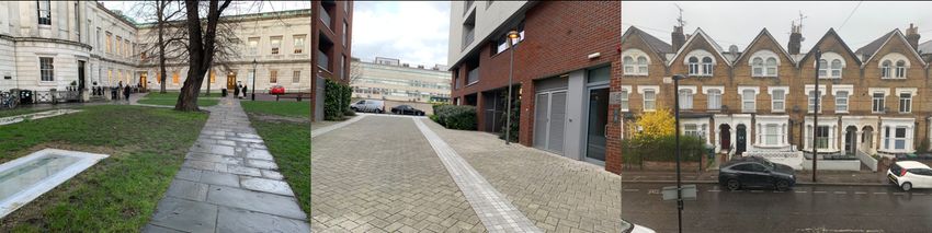
technology often used in such contexts (Huang et al., 2013); globally available and free-to-use (Langley,
Teunissen, & Montenbruck, 2017); and easily accessible given the high penetration of GNSS-enabled
smartphones (ESA, 2020). Furthermore, collecting data is straightforward as smartphones running the
Android operating system (currently comprising an 85% market share of new phones sold globally (IDC,
2020)) have allowed access to GNSS raw data since version 7.0 introduced in 2016 (Banville & Diggelen,
2016).
    Section 2 describes how a system would work in practice. A GNSS signal is transmitted from a
satellite at a known location (based on the signal’s timestamp) to a receiver with an estimated position
(either via GNSS or another navigation solution). If the signal is Line-Of-Sight (LOS) or multipath, it
may provide evidence that there are no intervening objects, and conversely non-line-of-sight (NLOS) or
blocked signals indicate an interaction with one or more obstacles. These data are processed by a map
building algorithm to generate the map, as discussed in section 4.
    Classifying GNSS signals between LOS (or multipath) and NLOS is a difficult problem even with
specialised equipment and software, but especially for smartphone receivers (Groves et al., 2013). In
this regard this paper proposes a GNSS-based map generating algorithm using the theoretical context
of computer vision techniques (section 3), which help to measure and assure the achievable quality, e.g.
accuracy. It is important to investigate if a bias in the signal classifier can affect map accuracy; and also
how the uncertainty due to the signal classifier can be reproduced in the produced map. GNSS mapping
works published to-date, as described in section 3, demonstrate different proposed algorithms but have
not yet addressed these points. Their results (Irish et al., 2014a, 2014b; Isaacs et al., 2014; Kim et al.,
2008; Rodrigues & Aguiar, 2019; Swinford, 2005; Weissman et al., 2013) rely on ad hoc justifications for
the chosen parameters or use non-generalisable training data-sets of labelled signals , which is addressed
in this paper..
    We introduce a new mapping algorithm (section 4) which is designed to be robust to bias in the
signal classifier, and to provide principled estimates of the uncertainty in the map output. We apply the
algorithm to empirical data collected in a range of urban environments within London and show that it
performs consistently across a wide range of initial signal classifiers (section 5).
    This paper is structured as follows: Section 2 describes the properties of GNSS required to understand
the remainder of the paper. Section 3 discusses 3D mapping and computer vision-based algorithms.
Section 4 proposes the 3D mapping algorithm using GNSS and section 5 implements the algorithm and
tests its performance. Section 6 discusses how the algorithm could be scaled up to a system built upon
contribution of data from volunteers at a city-wide scale.

2    Overview of GNSS
At any time, GNSS receivers may receive multiple radio signals transmitted from orbiting navigation
satellites. Guides to the principles of a GNSS system are widely available, for example the book "Gnss
data processing. volume 1: Fundamentals and algorithms" by Subirana, Zornoza, and Hernández-Pajares
(2013). It describes the GNSS signal as comprising a ranging code, also known as the pseudo-random-
noise (PRN) code, and navigation data. The receiver uses the ranging code to identify the transmitting
satellite and calculate the signal travel time from satellite to receiver, which is multiplied by the speed
of light to provide the apparent distance, known as the pseudorange (2013, p. 65). The navigation data
provides information on the satellite location along with supplementary information (2013, pp. 18–37).
Knowledge of satellite locations and pseudoranges allows the receiver to calculate its position and time
if enough satellites (usually 4 or more) are received (2013, pp. 18–37).
    The GNSS signals are used in 3 parts of the proposed 3D mapping system. Firstly, the GNSS
position solution can be used to estimate the receiver location and timestamp the signals, although this
is optional if other location estimates, including map or street view matching from the user inputs, are
available. Likewise the receiver’s own clock can be used if the time can not be calculated. Secondly, the
timestamp is used to obtain satellite positions from an authoritative reference such as the Navigation
Support Office at the European Space Agency (Mayer et al., 2019). Using an external reference, as
opposed to transmitted navigation data, provides the location of all satellites including those without
received signals. Lastly, the signal can be classified in relation to its propagation path, as detailed below,
using signal features such as the pseudorange and the Carrier-to-Noise ratio (C/N0 ). The C/N0 is not

                                                      2
directly part of the transmitted information but is a measurement by the receiver of the strength of the
received signal.
Like other radio-waves, GNSS signals can propagate to the receiver via a number of different paths.
Each path may involve different interactions with the environment, and each signal can be made up of
multiple path components. As illustrated in figure 1, this leads to classifying GNSS signals into 4 types:
• if the signal comprises one path without intervening obstacles, it is line-of-sight (LOS) (see figure
1, top-left),
• if the signal comprises one path that has been reflected or diffracted (the bending of a signal around
an edge) by obstacles, it is known as non-line-of-sight (NLOS) (see figure 1, bottom-right),
• if the signal comprises multiple components, which may include a LOS component or be entirely
NLOS, it is “multipath” (see figure 1, top-right),
• if no signal is received at all it is blocked (see figure 1, bottom-left).
Figure 1: GNSS signal types
For the purpose of 3D mapping, we must distinguish between a LOS component being present (LOS
or multipath with a LOS component) or absent (blocked, NLOS or multipath without a LOS component).
The identification of NLOS and multipath signals is the basis of many approaches to improving GNSS
positioning accuracy in urban locations, however reliably distinguishing between LOS and NLOS signal
components is a challenging problem (Breßler et al., 2016). Smartphone receivers are particularly prone
to receiving NLOS signals because their linearly-polarised antenna are equally sensitive to LOS and
reflected signals, whereas professional or traditional geodetic receivers are less sensitive to reflected
signals (Chen et al., 2012). At the same time, there are few techniques to identify NLOS signals using a
smartphone, because of hardware limitations relating to cost, size and power consumption (Groves et al.,
2013). Three main types of approach have been identified as suitable for smartphones, as detailed below.
The first set of approaches classify signals based on the environment, either using satellite elevation
on the principle that a low elevation signals are more likely to be blocked by obstacles (Yozevitch, Moshe,
& Weissman, 2016), or using a 3D city model as part of the position solution to jointly estimate position
and identify NLOS signals (Bourdeau, Sahmoudi, & Tourneret, 2012; Obst, Bauer, & Wanielik, 2012;
Peyraud et al., 2013; Wang, Groves, & Ziebart, 2013; Yozevitch, Ben-Moshe, & Dvir, 2014). This is
the inverse problem to creating a 3D map, hence such methods are not directly applicable to 3D map
creation.
3The second set of approaches identify signals that are likely to be NLOS because the indirect path
travelled makes their observed measurements, primarily pseudorange, inconsistent with other measure-
ments. These include calculating position solutions using different combinations of GNSS signals at the
same epoch (Groves & Jiang, 2013; Jiang et al., 2011); comparing measurements from other sensors in
an integrated positioning system (Soloviev & Van Graas, 2009); and comparing measurements against
prior position estimates using Kalman filters (Groves et al., 2013). Jiang et al. (2011) showed that con-
sistency checking has limited sensitivity for a typical (single-frequency) smartphone receiver as errors
due to the atmosphere’s effect can be as large as typical pseudorange errors. Furthermore, they depend
on the accuracy of other measurements, and in complex urban environments with many reflected signals
consistent pseudoranges can be generated by different subsets of NLOS observations (Jiang & Groves,
2012).
The third set of approaches use the carrier-to-noise ratio or derived measures to classify the signal.
These approaches are based upon the signal attenuating when interacting with obstacles, however the
effects of signal propagation are well-known to be more complex, as described by Molisch (2011). Re-
flections that cause NLOS signals vary depend on the reflecting surface and the angle of reflection. The
signal can be scattered on reflection from a rough surface, leading to a weaker signal in several directions
(2011, pp. 64–66), or specular reflection can be generated by a smooth surface, leading to a strong signal
in a particular direction (2011, pp. 49–51). Likewise, the effect on signal-strength depends on the degree
of diffraction (2011, pp. 54–63). Furthermore multipath signals have a larger variance in their C/N0
because of small-scale fading, the effect of relative phase on superposition of combining signals (2011,
pp. 27–29). As a result, it is possible for a specular reflection to be recorded as strong as or even stronger
than a LOS signal (Groves et al., 2013), and a GNSS signal can still be received at up to 5 degrees of
diffraction (Bradbury, 2007). Because of this, a smartphone GNSS receiver in an urban environment may
produce highly overlapping C/N0 distributions for LOS and NLOS signals (Wang, Groves, & Ziebart,
2015) and C/N0 can be an inaccurate NLOS classifier (Yozevitch, Moshe, & Weissman, 2016).
As a further source of difficulty, the C/N0 can also be affected by non-propagation errors: receiver
gain varies by smartphone make, model, and orientation (Chen et al., 2012); satellite transmission power
varies across constellations and the individual satellites due to different generations of specification and
a decrease in power as satellites age (Steigenberger, Thoelert, & Montenbruck, 2018); GNSS signals can
be affected by atmospheric conditions (Kintner, Humphreys, & Hinks, 2009) as well as features that are
temporary or too small to be included on a map, such as road vehicles or foliage on trees; and the human
body attenuates signals, as well as any bag or container in which the smartphone may be placed (Bancroft
et al., 2011). Many of these different errors cannot be detected or mitigated in a crowd-sourcing situation
due to the range of devices and varying methods of collection (Rodrigues & Aguiar, 2019). Therefore
any carrier-to-noise classifier calibrated under training conditions is likely to underperform when tested
in real world scenarios.
Applying machine learning methods to creating a NLOS classifier by combining features such as
C/N0 , pseudorange, elevation, and Doppler shift has been investigated using decision trees (Yozevitch,
Moshe, & Weissman, 2016), support vector machines (Hsu, 2017; Xu et al., 2020), nearest neighbours
and neural networks (Xu et al., 2018). However evidence for an improvement in accuracy against a
untrained Naive Bayesian classifier on C/N0 is mixed: Hsu (2017) showed an increase in accuracy from
67% to 75% and Yozevitch, Moshe, and Weissman (2016) showed a decrease in false positives from 45%
to around 20%, however other works (Xu et al., 2018; Xu et al., 2020) considering multiple situations
showed the simpler classifier had similarly or better accuracy in some situations. It has not been shown
that any improvements generalise beyond the original experimental settings.
The highly overlapping C/N0 distributions are suited to a probabilistic classifier. Irish et al. (2014b)
used a Bayes classifier based on a Rician distribution for multipath C/N0 and log-normal distribution
for NLOS, which are the canonical forms (Molisch, 2011). A quadratic spline form for the probability
density function was proposed by Wang, Groves, and Ziebart (2015). This paper proposes a 4-parameter
logistic curve (Healy, 1972) for the classifier form. It is a natural choice for a probabilistic classifier
as an extension of logistic regression, as discussed in more detail in section 5. In common with all
other approaches mentioned, its performance relies on the fitted parameters and is subject to the same
criticisms with respect to performance in a more general setting.
43 3D mapping as computer vision
Methods for generating 3D models of buildings using existing technologies are surveyed by Wang (2013)
and categorised as either image-based (for example photogrammetry) or range-based (for example LI-
DAR), or perhaps a fusion of the two. While GNSS is a range-based technology for the purposes of
navigation, the measured range is of the satellite and not of the environment we wish to map. However
by classifying each signal and considering the satellites’ relative positions from the receiver, it is possible
to derive an image, known as a skyplot, from the original measurements. This shows the set of satellite
observations from a receiver at a single epoch, as illustrated in figure 2. Similar to a silhouette image, it
only shows whether the direct ray to each satellite was open (when the signal is LOS or multipath with a
LOS component) or closed (when the signal is blocked, NLOS or multipath without a LOS component).
These images can then be used to generate a 3D map through techniques that have similarities to existing
image-based techniques.
Figure 2: Typical skyplot (azimuth-elevation graph) with classified signals
The earliest image-based approaches relied on knowing the position and calibrating parameters that
produced each image, known as the "camera poses" (Cyganek & Siebert, 2009), and primarily used
multi-view stereo (MVS) correspondence (Furukawa & Hernández, 2015), where stereographic corre-
spondence determines depth across a collection of overlapping images from multiple viewpoints. More
recent approaches use feature identification and matching across images, for example to recover camera
pose (Remondino & El-Hakim, 2006), however, a camera image is a complete set of observations across
a lens’ view, whereas a skyplot is an extremely sparse set of observations, which makes it impossible to
identify common features between two images. As common features cannot be identified between GNSS
images, a set of MVS techniques apply which use a negative deduction process: assuming the 3D-map
has a particular shape, checking how it appears in all the images, and iteratively improving the parts of
the object which are inconsistent with the images. Such MVS techniques have been shown to produce
sub-millimetre accuracy in lab testing (Seitz et al., 2006).
GNSS data does not allow a straight-forward application of existing MVS techniques because it is not
possible to measure the consistency of the 3D-map to the skyplots with the same precision. This arises
because unlike a picture, where parts of images can be compared by several continuous features such as
hue, intensity, and brightness, the skyplot only provides the outcomes of a binary classifier with limited
accuracy, which limits how consistency can be measured. The limitations of GNSS classification have
been discussed in detail in section 2. As a second problem, inaccuracy of receiver position may cause
the skyplots to be compared to the incorrect part of the 3D-map. The accuracy of the receiver position
may vary depending on how the position is estimated: GNSS position fixes are a natural automatic
positioning mechanism, but horizontal errors in built-up urban locations may be up to 50 metres for a
smartphone (Wang, Groves, & Ziebart, 2015); the receiver estimate could also be provided by the user,
leading to a semi-automated process subject to existing questions of volunteered data quality (Fan et al.,
52014).
While these problems may limit the detail of the produced 3D-map, GNSS mapping is an alternative
to existing 3D-map creation at the scale of a city, which historically utilises airborne methods focused
on coarse modelling with geometrically simple building and roof structures (Lafarge & Mallet, 2012;
Zebedin et al., 2006). CityGML, the Open Geospatial Consortium standard for 3D models, defines 5
increasing Levels Of Detail (LOD) with LOD 1 representing each building as an extruded block with flat
roof (Kolbe, 2009). LOD 1 is sufficient for many 3D mapping applications (Biljecki et al., 2015; Biljecki
et al., 2016) and is often a target for large scale 3D-map production (Dukai, Ledoux, & Stoter, 2019;
Girindran et al., 2020).
6Technique Scene Photo-consistency Visibility Shape priors Reconstruction algorithm Initialisation LOD
representation model requirement
Swinford Voxel – 1 N/A. NLOS measurements Not used 2.5D mapping Open signals used to progressively 2D map 1
(2005) metre cubes were ignored (columns remove voxels, as a form of space-
of occupied carving (Kutulakos & Seitz, 1999)
voxels must
have no gaps)
Kim et al. Voxel – N/A. LOS measurements Not used 2.5D mapping Counts of NLOS measurements Bounding box 1
(2008) unknown size ignored used to determine 2D footprint,
followed by cost-thresholding of
counts to determine height
Weissman et Voxel – Hinge-loss function for building Not used 2.5D mapping Counts of NLOS measurements Bounding box 1
al. (2013) unknown size height, using height of used to determine 2D footprint,
incorrectly classified signals building height estimated by
intersecting a vertical column minimising hinge-loss.
of voxels
Irish et Voxel – 4 Naive Bayesian probability of Probability None. Calculates posterior probabilities Bounding box N/A - surface
al. (2014a, metre cubes a voxel being occupied given of intervening for each voxel being occupied extraction
2014b) set of intersecting signals and a voxels being (modelling as a factor graph and unspecified
C/N0 probabilistic classifier unoccupied using a sum-product algorithm).
7
Similar technique to probabilistic
space carving (Broadhurst,
Drummond, & Cipolla, 2001).
Extended to allow for gaussian
noise in receiver location (Irish
et al., 2014a).
Isaacs et al. Voxel – Naive Bayesian probability of Not used None. Calculates probabilities for each Bounding N/A - surface
(2014) unknown size a voxel being occupied given voxel through an online learning box. extraction
Table 1: GNSS mapping algorithms
set of intersecting signals and a algorithm that applies the update Initialised unspecified
C/N0 probabilistic classifier to all voxels intersected by the using Irish et
signal, by stepping from their al. method
current value toward the photo-
consistency measure.
Rodrigues Voxel – 4 Binary classifer based on Not used None. Applies a trained classifier to each Bounding box 1
and Aguiar metre cubes C/N0 features of the set voxel, with intersecting signals
(2019) of intersecting signals, with weighted to allow uncertainty in
several machine learning receiver location
methods tried.
4PL-B 2D surface The likelihood of a building’s Not used 2.5D On a building-by-building basis: 2D map 1
(proposed mesh classifier given the observed set mapping. All maximum likelihood of the
in section 4) of signals (classified by signal buildings have associated four-parameter logistic
features) a single height regression with intersection height
parameter as the independent variableTo understand these limitations in practice, table 1 categorises existing GNSS-mapping techniques
and the algorithm proposed in this paper (section 4) against a taxonomy of MVS techniques intro-
duced by Seitz et al. (2006). This categorises an MVS algorithm by six fundamental properties: scene
representation, photo-consistency measure, visibility model, shape prior, reconstruction algorithm, and
initialisation requirements. As an additional category, we add the LOD of the produced map.
1. Scene representation is how the object geometry is represented. Primary types are voxel (a 3D grid
of pixels) or a 2D surface mesh. Many reconstruction algorithms require a particular representation.
2. Photo-consistency is a measure of the consistency between images to determine whether an object
reconstruction (which defines the projected images) is consistent with a set of images.
3. Visibility model is the method by which images are selected when evaluating photo-consistency
measures. It is important to exclude images where the object is occluded.
4. Shape priors guide the reconstruction algorithm to produce desired object characteristics such as
smoothness and maximal or minimal surface area or volume.
5. Reconstruction algorithm is the method of producing the reconstruction. Non-feature based meth-
ods typically work by minimising inconsistency cost either i) point-by-point (cost function defined
for each scene position and surface extracted based on a cost threshold); or ii) globally (cost function
defined for an object surface)
6. The initialisation requirement provides constraints on scene geometry. Many algorithms require
constraints (for example a bounding box) to function, and may obtain different solutions depending
on their initialisation.
Existing GNSS mapping algorithms seem to be relatively simplistic compared to existing MVS algo-
rithms. They are primarily distinguished by their varying approaches to photo-consistency, which reflects
the limitations discussed above. However, none of the approaches to date are satisfactory for generating
even an LOD 1 map. This is because the measurements of photo-consistency either ignore inconsistent
classifications (Kim et al., 2008; Swinford, 2005), or rely on a pre-specified signal strength classifier to
turn signal strength observations into a cost (Irish et al., 2014a, 2014b; Isaacs et al., 2014; Rodrigues &
Aguiar, 2019; Weissman et al., 2013), taking for granted that the classifier model is unbiased. The prob-
abilistic approaches of Irish et al. (2014b) and Isaacs et al. (2014) are potentially more robust because
they effectively give a higher weighting to observations with a more certain classification, however the
effect of model misspecification has not been investigated.
The algorithms also do not specify how uncertainty in the photo-consistency measure (due to signal
classification error and location error) should be reflected in the reconstruction algorithm. We emphasise
that the probabilistic approaches do not address this, as all posterior probabilities will converge to 0
or 1 with a large enough data set. The probabilistic approaches do not specify how a surface should
be extracted from the voxel probabilities, but probabilistic space carving is typically used with a cost-
minimisation approach, where cost would include negative likelihood as well as potential shape priors.
It is possible to reflect uncertainty through considering the sensitivity of cost to changes in the map,
however cost sensitivity is also a function of the chosen classifier and size of the data set , making such
approaches problematic. The algorithm we introduce in the next section seeks to address both problems
of bias and uncertainty.
4 GNSS-mapping algorithm
Our proposed GNSS mapping technique directly generates a 3D map by using it as a signal classifier
and solving the inversion problem given the observed signal data, similar to the MVS approach known
as statistical inverse ray tracing (Liu & Cooper, 2011). The technique is applied to a single building at
a time, using an existing 2D map to provide a building footprint. The set of GNSS observations that
intersect the 2D footprint form a dataset of (intersection height, signal features) pairs, as illustrated
in figure 3. The 3D map is extruded from the 2D footprint with the building height as an unknown
parameter. The technique uses a classifier based on signal features to label the GNSS signals and the
labelled signals are used as data to estimate the building height, as detailed below. This process is then
8Figure 3: Example of building data generated for 2.5D mapping from footprint intersection heights and
signal classifications
reversed with signals labelled as open or closed depending on whether they intersect the 3D building,
and these relabelled signals are used to train the signal classifier. This process iterates to improve the
building height estimates. Table 1 categorises the algorithm alongside existing approaches.
The proposed algorithm has three novel aspects relating to the photo-consistency problem:
• Firstly, it considers intersection height as a probabilistic classifier, using a four-parameter logistic
regression (4PL) as defined below as the classifier form for each building. This leads to a natural
interpretation of height uncertainty from the certainty of the classifier.
• Secondly, rather than generating the map by maximising its accuracy as a classifier, which creates
unwanted dependence on the bias of the signal feature classifier, it relates the map classifier pa-
rameters to the physical map, based on our understanding of the typical measurement errors of
the observations.
• Thirdly, once an initial map is generated, it is used to reclassify the signals and refit the signal
feature classifier, before repeating in a bootstrapping approach. This takes advantage of shape
priors to improve the map beyond observed data.
These aspects are discussed further following the details of the technique, which is set out as the following
pseudo-code 1. For simplicity it assumes the only signal feature used for classification is the carrier-to-
noise ratio, however any signal classifier could be used, as long as it is class-conditionally independent of
9height, and section 2 contains more detail on potential classifiers.
Algorithm 1: 4PL-B algorithm
function SignalClassifier (param,ss):
/* signal strength classifier, with heuristic initial parameters */
if ss=n/a then return 0 else return Pr(ss);
function 4PL ((a,b,c,d),h):
/* four parameter logistic regression associated with the building, with
intersection height as the independent feature used to classify signals */
return Pr(h);
input : A set X of observation tuples (y, ss, h) for a building
y: signal label (initially blank)
ss: C/N0 (n/a if blocked)
h: intersection height
output: Parameters (a, b, c, d) of 4PL
c + 1.5/b: height point estimate
(c, c + 3/b): height range estimate
repeat (
1 SignalClassif ier(param, ss) > 0.5
for (y, ss, h) ∈ X do y ←− ;
0 o0 wise
(a, b, c, d) ←− maximum likelihood
( estimates for 4PL given X
1 h>c
for (y, ss, h) ∈ X do y ←− ;
0 o0 wise
param ←− maximum likelihood estimates for SignalClassifier given X
until (a, b, c, d) have converged;
A 4PL extends logistic regression to consider asymptotic probabilities other than 0 or 1(Healy, 1972).
It has the following univariate form:
a−d
Pr(x) = d +
1 + exp(−b(x − c))
Where a and d are the upper and lower asymptotes, respectively, and b and c are the standard linear
coefficients in x. The 3D mapping algorithm uses the maximum likelihood estimates of the 4PL parame-
ters, which can usually be obtained through standard optimisation methods although the EM algorithm
has been proposed as a superior alternative (Dinse, 2011). Gradient descent methods (Ruder, 2016) can
also be used to optimise the parameters, which raises the possibility of using stochastic gradient descent
on the classifiers and performing batch-updates on each classifier in turn, in order to allow the 3D map
to be updated over time as new data is collected.
The use of the 4PL is integral to the proposed technique as the parameters have a physical inter-
pretation relating to the observation errors, as illustrated in figure 4. Without these errors, an idealised
height classifier would be a step function, with zero probability of open signals for intersections below
building height and probability of one above building height.
The 4PL asymptotes reflect signal classification error, where a is the positive predictive value, or
precision, of the signal classifier and d is the false omission rate (equal to 1 minus the negative predicative
value). It is important to clarify that these are primarily the error rates of the signal classifier which has
noisily labelled the data, and not the error rates for the map classifier against the true unknown labels.
The scaling parameter b relates to the uncertainties in building height, for reasons including unmod-
elled effects such as diffraction effects and the complexities of building roofline, and measurement errors
such as incorrect intersection height due to receiver location errors. A gentle slope indicates a lower level
of certainty in building height as the effect of height on signal class is prolonged, whereas a steep slope
indicates more certainty due to an abrupt height effect.
The inflection point c, relates to the unknown building height. The b and c parameters generate a
height estimate of c + 1.5/b with a range between (c, c + 3/b) as explained below.
10Figure 4: Four-parameter logistic regression
The rationale for this approach is that the GNSS received signal strength and intersection height
can be treated as class-conditionally independent, with the exception of diffraction effects and height
errors. Class-conditionally independent means that within a signal classification (open or closed) the
signal strength is independent of the intersection height: for open signals (where the signal intersection
height is above the building height) there is a LOS component which does not interact with any obstacles
and this is unaffected by intersection height; likewise, for closed signals (where the signal intersection
height is below the building height), the LOS component has been blocked and this is unaffected by the
intersection height.
This is a generalisation: the contribution of multipath and NLOS components as well as any effects of
unmapped objects on LOS components will depend on position but with a reasonable spatial distribution
of observations around the building the dependence on height is presumed to be ignorable; the algorithm
also assumes that the blockage of signals by other buildings (which will have a height dependence) does
not have an effect, but this is a similar approach to other MVS algorithms, which correct for this problem
using a visibility model rather than in the photo-consistency measure; the remaining dependence comes
from diffraction effects and height errors, which are explicitly accounted for in the algorithm.
When diffraction effects and height errors are negligible, the class probability (which is measuring
the consistency of the signal strength classifier and map classifier) is independent of intersection height,
as represented by the asymptotes of the 4PL with zero gradient. As the intersection height approaches
the building height from either direction, a growing proportion of signals may be misclassified by the
map due to height errors. This occurs when the intersection height is between the modelled building
height (which is modelled as uniform across the building) and the actual building height, which varies
across the building with roofline complexity, or conversely, when the actual building height is between
the measured and actual intersection height due to receiver location errors.
These effects lead to a slope between the asymptotes instead of a step, however the effect of intersection
height errors should be symmetric, and therefore not affect c, the inflection point of the 4PL. The effect
of non-uniform building height will shift c to the average building height across the observations, which
should be a good approximation of the true average building height with spatial diversity of observations.
On the other hand, diffraction effects depend on the degree of diffraction of the signal which depends
on both the distance of the receiver as well as the difference between building height and intersection
height. As a simplification, the algorithm assumes that the height difference is a proxy for the degree of
diffraction, and as this decreases the signal attenuation lessens, leading to an increasing number of LOS
classifications.
This is an asymmetric effect, as it only has an effect when the intersection height is below the
11building height. This has the effect of shifting the inflection point c below the true building height,
therefore the building height should be above the inflection point and towards the upper asymptote.
Given the uncertainty of the relative magnitude of intersection height error and diffraction effect, we
conservatively suggest a point estimate of c + 1.5/b and range between (c, c + 3/b), which represents the
50% to 95% percentile of the distance between the asymptotes.
It follows from this formulation that our estimate does not impose any additional assumptions on
the signal strength classification accuracy, whereas a solution provided by a cost-minimisation approach
depends on the signal classification model being an unbiased classifier. The proposed approach provides
a height estimate that is robust to model bias and also provides a measure of uncertainty in the height
due to the underlying measurement uncertainty.
In order to improve the classification accuracy, this paper builds upon the class-conditionally indepen-
dency of GNSS signal strength and height, and uses a co-training approach to label data more confidently
through an iterative process. Blum and Mitchell (1998) introduced co-training as a form of disagreement-
based semi-supervised learning, which uses a pair of binary classifiers to label a dataset by iteratively
applying each classifier and using the most confidently labelled instances as training data for the other
classifier. In the straightforward bootstrapping approach we take here, we consider all labelled signals
as training data, and stop when the map classifier parameters converge. This does not require the two
classifiers to have consistent labels, but indicates that the classifiers are class-conditionally independent.
5 Implementation
To verify the accuracy of our proposed algorithm, we estimated the height of a range of buildings
in different urban environments in greater London by collecting GNSS observations nearby and using
them as inputs into the proposed algorithm. The next subsections describe the experimental setup and
algorithm results.
5.1 Experiment
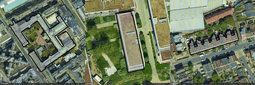
Urban environments in greater London vary in use, street width, building height and density, and
construction material. To compare algorithm performance in different environments, three representative
buildings are presented which cover a wide range of building heights, construction materials, and sky
visibility(see Figure 5). The first is the main estate of University College London, the second is a block
of flats (Goodchild Road) in an urban canyon, and the third is a terrace of houses (Hermitage Road) in a
residential setting. The university estate is a building of significant height and mass, built primarily from
stone in the 19th century, with nearby open space allowing spatial diversity of data collection. The block
of flats represents modern inner-city construction: it is of moderate height in a high-density location,
built within the last 20 years from reinforced concrete with a brick and glass facade, the observations were
made from a narrow pedestrianised street with visibility to the sky only at high elevations. The terrace
is low density and low height, it is brick-construction from early 20th century, and the observations were
made with a restricted collection protocol from the far side of the street to maximise the number of
received low elevation signals.
A Samsung Galaxy 10 running the Android 10.0 operating system was used as the GNSS receiver.
It supports the four major GNSS constellations: Global Positioning System (GPS), GLObal NAvigation
Satellite System (GLONASS), Beidou, and Galileo. Multi-constellation receivers such as these ones are
now standard and embedded in many mobile devices (ESA, 2020), and result in a device typically having
potential LOS to 30 to 50 GNSS satellites above the horizon at all times. As described further in section
6, Android phones allow access to "raw" GNSS data for all signals, along with associated GNSS receiver
position solutions. We developed a recording app based on Google’s GNSS Logger (Banville & Diggelen,
2016) that accesses the raw data for the position solution and satellite identifier, used to determine
the direct signal path, and the carrier-to-noise density, used to classify the signal. The app also allows
manual recording of observer locations.
For each site the receiver was placed in a static location and measurements were recorded as a
stream of data measured at 1Hz frequency for a duration of around 30 minutes. This was undertaken
twice at UCL, and 5 and 6 times at the Hermitage Road and Goodchild Road sites respectively, at
12Figure 5: Experiment locations above, and photos below. From left to right: UCL, Goodchild Road,
Hermitage Road. The outlined polygon is the building footprint according to OS Mastermap, this was
used in the algorithm with the background map tile for illustration only. Background map tile: Google,
©2021 Bluesky, CNES/Airbus, Getmapping plc, Infoterra Ltd & Bluesky, Maxar Technologies, The
GeoInformation Group
different locations and times of day to allow the satellite geometries to change. The varying frequency of
measurements across sites were to provide similar numbers of intersecting signals across the different sizes
and shapes of floorplates. The dataset is summarised in table 2. The observer locations were manually
inputted based on a visual determination against a small-scale map, with an estimated location error of
below 2 metres. Results are presented in this paper for both the more accurate manually input locations
and the automatic GNSS position solutions
Table 2: Summary of collected data
Recorded Number of signals observed
Site ID Epochs
Recorded Blocked Total Intersecting
UCL 3,558 88,633 5,284 93,917 88,106
Goodchild Rd 8,136 227,658 21,718 249,376 95,362
Hermitage Rd 8,350 26,094 310,618 336,712 100,884
For each observation time, all satellite positions were retrieved using information on satellite orbits
freely available from the Navigation Support Office at the European Space Agency, which allowed the
dataset to be expanded to blocked signals for all receiver-supported constellations. An elevation filter
was applied to remove low elevation signals, as these are often blocked by background and unmapped
objects. The elevation filter was set at 10 degrees for the UCL and Goodchild Road sites, and 0 degrees
for the Hermitage Road site, where the recordings were made from a relative distance and position such
that many low elevation signals were received. As a last step, observations with a satellite elevation above
85 degrees were also removed, because at these elevations trigonometry implies errors in the observer’s
horizontal position are magnified 11 times or more in calculations of intersection height, making the data
unacceptably poor quality. The elevation was calculated with respect to the tangential plane on the
WGS84 ellipsoid.
13The building footprints were obtained from the Ordnance Survey GB, Great Britain’s national map-
ping agency. Ordnance Survey’s MasterMap (Ordnance Survey, 2020c), provides the benchmark map
for the country, in terms of reliability and accuracy. GNSS elevation data is collected by a receiver with
reference to the WGS84 ellipsoid. It was converted using accurate transformation grids, as described in
Ordnance Survey (2020a), to the coordinate reference system used by OS Mastermap: British National
Grid for horizontal coordinates and Ordnance Datum Nelwyn (ODN), a local geoid, for heights. Figure
6 illustrates the conversion between ODN and WGS84 and the relation between absolute building height
and relative building height from terrain. The results in this paper are reported as absolute heights with
reference to ODN. It also illustrates how building heights in a LOD 1 model depend on the choice of
geometric reference: the lowest or highest point of a roof may be used, or any ad-hoc point or average
of points in-between (Biljecki et al., 2016)
Figure 6: Building height definitions
The building heights, shown in table 3, were obtained from OS MasterMap (Ordnance Survey, 2020b)
where available, and Google Earth (Google, 2020), and represent the minimum and maximum heights
across the buildings, with the UCL building being particularly complex with a large dome and varying
levels. For the UCL building, the adopted height in the paper is the height of the Library entrance hall,
which we believe is representative of the larger building. While this is a subjective choice, the value of
our algorithm lies in its consistent results over a range of starting conditions, and this conclusion holds
for any reasonable adopted height for the UCL building. We adopt the midpoint of the height range
as the ground truth height.1 Table 3 also shows the indicative ground elevation and relative building
heights, determined using the OS Terrain 5 Digital Elevation Model (Ordnance Survey, 2020d).
Table 3: Building heights
Site UCL Goodchild Road Hermitage Road
OS Height (min-max) 43.8m - 47.1m - -
Google Earth (min-max) 44.0m - 47.0m 47.0m 33.0 - 35.0m
Representative LOD1 height 46.0m 47.0m 34.0m
Indicative ground elevation 26.0m 31.0m 24.0m
Indicative relative building height 20.0m 16.0m 10.0m
To calculate the intersection height at which the LOS component of each signal would intersect the
building, it was assumed that the signal travelled in a direct line with respected to the projected plane
coordinate system. This neglects earth curvature, however for all plausible observations with at most
141km distance between an observer and a building, the effect is only 8cm. Likewise curvature of the signal
due to atmospheric diffraction is less than 0.8 arcseconds, which equates to less than 1cm effect at 1 km
(Möller & Landskron, 2019).
5.2 Results
5.2.1 Signal Classifier
GNSS mapping algorithms rely on a signal classifier to predict whether a signal was open (LOS or
multipath with a LOS component) or closed (blocked, NLOS or multipath without a LOS component),
and the performance of the signal classifier plays an important role in the quality of the produced map.
It is important to investigate if bias and uncertainty in the signal classifier affects the produced map.
This paper classifies individual signals by their C/N0 through implementing a 4PL probabilistic
classifier, with the most likely classification being assigned. The form of classifier was chosen based on the
results of Wang, Groves, and Ziebart (2015). They proposed a quadratic spline form however we suggest
that a 4PL has advantages of monotonicity and smoothness that make model fitting through optimisation
more robust. It is worth reminding readers that this has no connection to the 4PL used in the map
classifier, but happens to have a form that is a good fit to the observed data. More complex alternative
classifiers are discussed in section 2, and use additional features available as raw data. Likewise, the C/N0
classifier could be extended to model ionospheric and tropospheric effects as well as taking into account
specific device receiver gain and satellite transmission power. These complexities were not implemented
in the paper, as the advantage of the proposed algorithm is that the generated map is relatively robust
to the accuracy of the classifier.
To assess the performance of the signal strength classifier, the ground truth building heights were
used to label the dataset. The C/N0 distribution of open and closed signals is shown in figure 7. The
two signal classes have distinct but overlapping distributions, demonstrating the difficulty of accurately
predicting class. Predicting closed signals at low signal strengths can be more straightforward than open
signals at high signal strengths, based on the overlap of the two distributions. Almost no signals were
received with a C/N0 of less than 10 dB-Hz, which was an expected effect marking the cutoff below
which the signal is too weak to be registered by the receiver. There is an anomalous peak of observations
just above this level, which we are unable to explain with any certainty.
Figure 7: Distribution of received signals
A probabilistic 4PL classifier was trained on the dataset pertaining to the UCL building, and tested
on the data from the other locations. Figure 8 illustrate how the varying observational settings affect the
15relationship between LOS probability and signal strength. which decrease the performance of trained
signal classifiers. This leads to a stark divergence in performance of the signal strength classifier between
training and test data.
Figure 8: Distribution of received signals
The 4PL signal classifier fits the observed proportions for the training data relatively well, with a
Mcfadden’s R2 of 70.7% , but is wrongly parameterised for the test data, with a Mcfadden’s R2 of
18.9%. The performance of the 4PL across the dataset is shown in table 4, which cross-tabulates the
true labels against the predictions obtained by the trained 4PL, using a 50% probability threshold to
label classes. Figure 9 illustrates the effect on accuracy of changing the classification threshold. The
performance of a single classifier across the combined test locations can only be improved marginally
by optimising parameters. As discussed in section 2, these parameters are device and location specific,
making it difficult to generalise the classifiers.
Table 4: Test data cross-tabulation by predicted (C/N0 ) and actual (Height) class. Height n/a indicates
the signal did not intersect the building.
Height Class
Open Closed n/a Total
C/N0 Open 40,683 27,474 95,062 163,219
Class
Closed 23,750 104,339 294,780 422,869
Total 64,433 131,813 389,842 586,088
16Figure 9: Signal classifier performance with varying classification thresholds. Highlighted classification
value represents the 50% probability class threshold estimated by the trained 4PL
5.2.2 Map Algorithm
To assess the map algorithm, it was applied to each location’s dataset. To evaluate the impact of a
misspecifed signal classifier, it was repeated using a range of parameters for the initial signal strength
classifier. For comparison, the same signal classifier was used in the non-bootstrapped 4PL algorithm, the
Weissman et al. (2013) hinge-loss method, and a Bayesian probabilistic method of maximising likelihood
similar to Irish et al. (2014a), albeit applied to the entire dataset rather than to each voxel. The signal
strength 4PL was initialised with the same initial parameters (a: 0.9, b: 0.2, d: 0.1) except for the
inflection point, c, which ranged from 20-40 dB-Hz in 1 db-Hz increments. This generated a range of
50% probability classification thresholds from 20 to 40 dB-Hz, which we believe is a plausible range: the
thresholds for our datasets were between 23 and 40 dB-Hz respectively, and other works have ranged
from 23 dB-Hz (Wang, Groves, & Ziebart, 2015) to 37.5 dB-Hz (Yozevitch, Moshe, & Weissman, 2016).
The bootstrapping algorithm was stopped at the lower of 10 iterations and fewer than 1% of the labels
having changed between two iterations of the map classifier.
Figure 10 shows the algorithms results when applied to the datasets with the manually inputted, more
accurate, receiver locations. The 4PL-B algorithm converged to a solution at all 20 starting conditions
at the UCL and Hermitage Road sites, and 15 out of 20 at the Goodchild Road sites. The other non-
iterative algorithms always generated a solution (not always shown in the figure due to being outside
the limits of the y-axis) however is not necessarily advantageous to return a low quality estimate. Table
5 show the root mean square error for each algorithm and site across all 20 different initialisations. The
4PL-B algorithm is more accurate by an order of magnitude due to its consistency.
17Figure 10: Mapping algorithm results with varying signal strength classifiers
Table 5: Root Mean Square Error of mapping algorithms
UCL Goodchild Hermitage
Road Road
Manually input locations
4PL-B 1.4m 1.4m 0.8m
4PL 2.1m 11.7m 7.8m
Hinge-Loss 5.6m 7.4m 20.6m
Bayes 8.6m 24.9m 18.7m
GNSS position solutions
4PL-B 0.6m - 0.8m
4PL 1.4m 28.7m 19.5m
Hinge-Loss 5.6m 10.1m 9.9m
Bayes 7.6m 29.9m 31.6m
Calculated for each site across all twenty initialisations. 4PL-B results were
excluded where the algorithm did not converge: 5 results for the Goodchild
Road site using manual locations; all results at Goodchild Road using GNSS
locations; and 4 at the Hermitage Road site using GNSS locations.
Unlike the 4PL-B algorithm, which provides consistent results regardless of initialisation, results for
the other methods depend on choice of initialisation. The Weissman hinge-loss algorithm increases su-
perlinearly with initial classification threshold and nothing can be usefully inferred without a knowledge
of the optimal classification threshold for the dataset. The Bayesian algorithm results increase mono-
tonically, not smoothly but with stepped increases and relatively stable clustering around certain values.
It requires less precise knowledge of the optimal classification threshold but the initial classification
must still be relatively accurate otherwise the algorithm can generate wildly inaccurate results. The
non-bootstrapped 4PL algorithm performance varies by location. In less challenging locations (UCL) it
18performs consistently, but in more challenging locations it requires a relatively accurate starting point,
similar to the Bayesian approach.
The difficulty that the non-bootstrapped 4PL algorithm has in certain locations appears to be due to
the overall balance of collected data. In the two more challenging locations, the environment and data
collection protocol was such that most of the data was blocked (Goodchild Road) or open (Hermitage
Road). The model is fit to the data as a maximum likelihood estimate with the simplifying assumption
that signal strength is independent of height within a class. However there will always be weak patterns
of height dependency and signal strength, and if most of the data is within the same class then the
model fits weak patterns within the class, due to the weight of data, rather than the stronger pattern
across classes which is only present in a small quantity of data. Preliminary work suggests that improve-
ments can be obtained by filtering and rebalancing the data based on the distribution of intersection
heights. Improvements to the 4PL algorithm could help broaden the conditions of convergence for the
bootstrapped algorithm.
Table 6 shows the 4PL-B algorithm measure of uncertainty around the building height based on the
steepness of the 4PL curve, compared to the true height. The algorithm uncertainty is in accordance
with the relative complexity of the building shape: Goodchild Road is a simple flat roof, Hermitage Road
is a terrace with pitched roofs, and UCL has a complex roof shape.
Table 6: Uncertainty reported by 4PL-B algorithm
UCL Goodchild Hermitage
Road Road
Manually input locations
min-max heights 41.9m - 47.4m 45.4m - 45.8m 33.4m - 36.2m
uncertainty range 5.5m 0.4m 2.8m
GNSS position solutions
min-max heights 41.5m - 49.5m - 30.7m - 38.8m
uncertainty range 8.0m - 8.1m
Google Earth
min-max heights 44.0m - 47.0m 47.0m 33.0 - 35.0m
uncertainty range 3.0m 0.0m 2.0m
Google Earth uncertainty for UCL height is that of the Library entrance hall.
The entire building has a height which ranges between 26.0m - 58.0m (Ordnance
Survey, 2020c).
The process was repeated on the data using the GNSS-provided latitude and longitudes rather than
the manually input locations. This increases location errors but fully automates data-collection. We
re-ran results using the GNSS-provided latitude and longitudes, and setting the altitude for all signals
as 1m above ground level for the experimental location, using the OS Terrain 5 Digital Elevation Model
(Ordnance Survey, 2020d). By using digital elevation models, it is possible to avoid typically large
vertical errors in GNSS positioning, which can create intersection height errors. The results are shown
in Figure 11 and Table 5. The 4PL-B algorithm perform relatively accurately at the Hermitage and
UCL sites, where satellites were visible at low and moderate elevations but failed completely for the
Goodchild site, where only high elevation signals were visible. This is understandable because when only
high elevation signals are visible, the GNSS position errors are typically larger due to geometric dilution
of precision, and this is compounded because the high elevation also increases the effect of horizontal
error on calculated intersection height. The other algorithms showed the same effects. The uncertainty
reported by the 4PL-B increased with the GNSS solutions (table 6) highlighting that the algorithm is
able to reflect the quality of the position data in its reported results.
19Figure 11: Mapping algorithm results with GNSS position solutions
6 Discussion
This section considers how the GNSS mapping algorithm could be scaled up to a VGI system on a
city-wide scale. It discusses how a system could be implemented; how the algorithm could be extended
to consider occlusion; whether the approach extends to a higher LOD; and the role of location errors.
The key advantage of a GNSS mapping approach is that participation in the VGI project is straight-
forward and almost entirely passive. The necessary data is already continually collected by GNSS-enabled
smartphones to facilitate positioning and the use of location-based services. Since version 7.0 introduced
in 2016, the Android operating system allows access to “raw” GNSS data through the android.location
Application Programming Interface (API) (ESA, 2017), i.e. any installed mobile applications (app) with
user permissions can use the GNSS raw data. The API usually provides signal observations at a 1Hz
frequency, and consequently a single smartphone can generate above 100,000 signal observations an hour,
including signals that were expected to be received but in practice were blocked due to obstacles between
the satellites and the receivers such as buildings.
To implement a large-scale VGI system primarily requires the creation of Android mobile app, which
is installed by a participant, and for it to run as needed in the background, with the option of the
user manually inputting locations. The app can then periodically upload data to a central server for
processing. GNSS data provided through the API includes all the information required by the various
signal classifiers described in Section 2: the GNSS navigation message, from which the satellite and
its azimuth and elevation can be identified, along with typical GNSS observables such as pseudorange,
carrier phase, precise timing and doppler shift. The carrier-to-noise ratio is also available. Further
study is planned to develop a VGI mobile application and address pertinent questions e.g. privacy,
incentivisation and participation.
The presented algorithm considers signals being blocked by a single building. On a larger scale,
additional occlusion may occur. This could be due to a taller building further away from the receiver in
the same direction, or unmapped objects (e.g. buildings due to a outdated basemap; or trees and other
street furniture) between the receiver and the building of interest. This would present itself as greater
uncertainty and error in the height estimate due to the occlusion effects.
Spatiotemporal diversity of data collection should mitigate many of these errors, as the occlusion will
vary based on the receiver position and signal azimuth and elevation. This suggests a more granular
20You can also read