Advanced Studies in Applied Statistics (WBL), ETHZ Applied Multivariate Statistics Spring 2018, Week 8 - Lecturer: Beate Sick
←
→
Page content transcription
If your browser does not render page correctly, please read the page content below

Advanced Studies in Applied Statistics (WBL), ETHZ
Applied Multivariate Statistics
Spring 2018, Week 8

                                    Lecturer: Beate Sick
                                           sickb@ethz.ch
 Remark: Much of the material have been developed together with Oliver Dürr for different lectures at ZHAW.
                                                                                                              1
Topics of today

•   Purpose of the model (explain/predict) makes a difference

•   Descriptive modeling – focusing on model coefficients
     – Interpretation of the model coefficients

•   Causal modeling - scratching the surface

•   Predictive modeling – focusing on predicted outcomes
     – Evaluation
     – Calibration
     – Shrinkage

•   Regression to the mean in test re-test situations

•   Practical considerations

                                                                2
Where does the term “regression” come from?

The concept of regression comes from genetics
and was popularized by Sir Francis
Galton during the late 19th century with the
publication of Regression towards mediocrity in
hereditary stature.

Galton observed that extreme characteristics
(e.g., height) in parents are not passed on
completely to their offspring. Rather, the
characteristics in the offspring regress towards
a mediocre point (a point which has since been
identified as the mean).
Source: https://en.wikipedia.org/wiki/Francis_Galton

                                                       3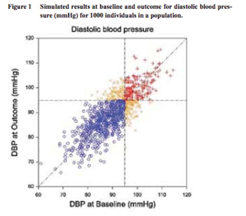
For what purpose do we develop a statistical model?
Description:
Describe data by a statistical model.
Explanation:
Search for the “true” model to understand and causally explain the
relationships between variables and to plan for interventions.
Prediction:
Use model to make reliable predictions.
4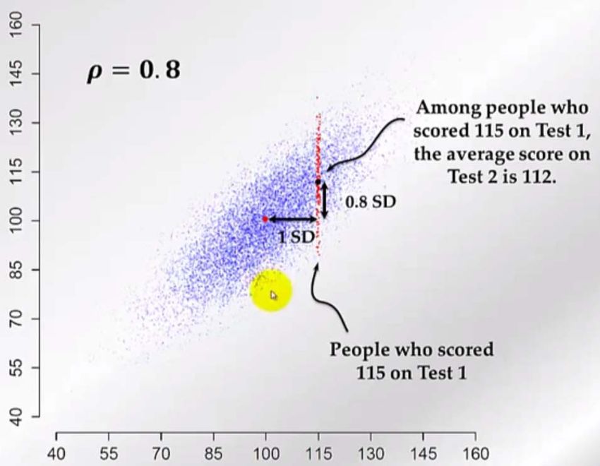
Linear regression – the mother of all statistical models
as used in descriptive modelling
Model for the c onditional probability distribution
y i = 0 + 1 xi 1 i
CPD: YX i =(Y|X i ) ~ N( xi , ) 2
E YX i xi =( |X =x i )= 0 + 1 xi1
Yx
x is given 2 is independent of Var(YX i )=Var(Y|X i )=Var( i ) 2
x by the model the predictor values
i i.i.d. ~ N (0, 2 )
MPD
CPD
CPD
CPD
Y is continuous and can have
probability distribution
an arbitrary marginal
contiuous
Y ~ Varbirar y
(Y|X i ) ~ N( xi , 2 )
5
Example for a multiple regression model: HDL model

              Estimate Std. Error t-value           Pr(>|t|)
 Intercept      1.16448   0.28804    4.04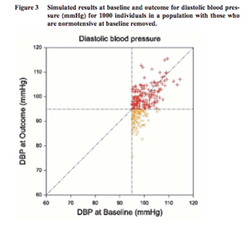
On the meanings of the coefficients and p-values

 SKINF (skinfold thickness) alone probably is associated. However, its p=0.42 says
 that it provides no additional information that helps to predict LogHDL, after
 accounting for other factors such as BMI *).

 The p-value and also the coefficient-value of a predictor depend i.g. not only on the
 association with the outcome variable but also on the other predictors in the model.

 Only if all predictors are independent multiple regression leads the same p-values
 and coefficients than p simple regression each with only one predictor.

 *) In
     a RF importance plot, SKINF would probably get a high importance, since it is good predictor leading to
 good splits with good chances to be chosen as split variable especially if BMI is not in the randomly sampled
 subset of potential split variables ‐> importance in classical RF ≠ significance in mul variate regression
 (conditional tree based trees from the party package leads more to importance measures that have a more
 similar interpreted as variable influences from variables in regression models).
                                                                                                                 7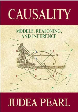
Poisson regression revisited
CPD: YX i =(Y|X i ) ~ Pois( xi )
log E (Yxi ) log(xi ) 0 1 xi1
Yx 0 , x E (Yxi ) xi e 0 1xi1 =e 0 e 1xi1
Var(Yxi ) xi
The predicted value of the Poisson regression gives
the only one parameter of the CPD: x that depends (Y|X i ) ~ Pois( xi )
on the predictor values. We have no error term in the regression
Xk
formula since the uncertainty of the outcome (counts) is given by the P (Y | X) k e X , k 0,1, 2,...
probabilistic Poisson model Pois(x) k!
3000
2000
count
discrete
Y ~ Varbi ra ry
1000
500
(Y|X i ) ~ Pois( xi )
0
0 10 20 30 40 50
x
8
Poisson regression: interpretation of coefficient
In Poisson regression, we are modelling the log‐expected counts of events
log E (Yi ) log(t i ) 0 1 xi1 ... p xip
E(Yxk 1 )
k =log E(Yx 1 ) log E(Yx ) log : log-count-ratio
k k E(Yx )
k
E(Yxk 1 )
T xk 1
log log : log-rate-ratio
E(Yxk ) x
T
k
E(Yxk 1 )
nobserved P(event) xk 1
log log : log-risk-ratio
E(Y )
xk P (event) xk
nobserved
Thus is the ratio of the counts or count‐rate or risk‐ratio w.r.t to the
reference level or when the explanatory variable xk is increased by 1 unit
and all other variables hold fix.
– If k =0, the counts are equal at all xk levels ( =1)
– If k >0 , the counts increases as xk increases ( >1)
– If k < 0 , the counts decreases as xk increases (
Logistic regression revisited
CPD: YX i =(Y|X i ) ~ Ber( p xi ) pxi
log 0 1 xi1
1 px
Yx {0,1} , p x [0,1] i
e 0 1xi1
E (Yxi ) E (Y 1| X xi ) pxi
The predicted value of the logistic regression gives the 1 e 0 1xi1
only one parameter of the CPD: px that depends on Var(Yxi ) pxi (1 pxi )
the predictor values. We have no error term in the regression
formula since the uncertainty of the outcome (counts) is given by the
probabilistic Bernoulli model Bernoulli(px)
p x 0.1 p x 0.5
p x 0.95
px , y=1
P (Y | X x)
1 px , y=0
p x 0.95
#(y 1)
n , for y=1
P (Y)
#( y 0) , for y=0 p x 0.5
n
p x 0.1
0 1 xi1
10Logistic regression: interpretation of coefficient
^
p
log log oddsi 0 1 xi1 ... p xip
1 p
odds xk 1
k = log(odds x 1 ) log(odds x ) log log(OR x x 1 )
k k odds x
k k
k
e k OR xk xk 1
– Thus gives the OR w.r.t to the reference level or when the explanatory
variable xk is increased by 1 unit and all other variables hold fix.
– If k =0, the odds (and probability) is equal at all xk levels ( =1)
– If k >0 , the odds (and probability) increases as xk increases ( >1)
– If k < 0 , the odds (and probability) decreases as xk increases (Descriptive modeling has a long tradition in statistics
“Descriptive modelling is aimed at summarizing or representing given data in a
compact manner. …the reliance on an underlying causal theory is absent”
Source: Shmueli 2010
“Considerations of causality should be treated as they have
always been in statistics: preferably not at all;
But if necessary than with great care"
Terry Speed, president of the Biometric Society 1994‐95
Especially we cannot use coefficients in linear regression model to predict
how the outcome y would change if we make an intervention and increase
a certain predictor by one unit (we make no intervention on all other
predictors neither do we control them).
12Causal modeling
13Sidetrack: Causal effects are best derived from randomized trials
?
Treatment is assigned randomly
→ differences of the outcome between both treatment groups is due to the treatment:
causal effect = intervention effect
→ appropirate regression model: ~ 14Judea Pearl introduced causal reasoning into statistical modeling
of observational data
Key idea: use causal graphs and backdoor
criterion to determine for which covariates
we should adjust to get a causal model.
ACM Turing Award 2011: “For fundamental contributions to artificial
intelligence through the development of a calculus for probabilistic and
causal reasoning."
15Pearl’s ideas were picked up and extended by famous statistics groups
P. Bühlman (ETH): “Pure regression is intrinsically the wrong tool”
(to understand causal relationships between predictors and outcome and
to plan interventions based on observational data)”
https://www.youtube.com/watch?v=JBtxRUdmvx4
16Sidetrack: Causal effects can also be derived from observational
data when using Pearl’s backdoor criterion is fulfilled
When can the regression coefficient in a model be interpreted as causal effect?
We need to adjust with an appropriate set SB of covariates Vi (e.g. all parents of X) which
would be sufficient to close all backdoor paths from intervention X to the outcome Y
outcome ~ predictor +
V S
Vi outcome ~ predictor + parents(predictor)
i B
17Predictive modeling
18Retrospective vs Prospective modeling
Descriptive modeling is retrospective:
the model is used to describe the collected data.
Explanatory modeling is retrospective – the model is used
• to test an already existing set of hypotheses
• to estimate the causal effect of a predictor on the outcome
for both cases appropriate data that were collected for this purpose
Predictive modeling is prospective (forward-looking):
the model is constructed for predicting new observations.
Model assessment of retrospective models is done on data used to build the model.
Model assessment of prospective models is done on new data.
19Let’s simulate some data and split them in train and test set
…
20Let’s fit a linear regression model for descriptive modelling
21Statisticians descriptive model check: residual analysis
Residual plots look o.k., what is expected since true model is fitted to simulated data.
22Poor man’s descriptive model check: observed vs fitted
main diagonal
fitted regression line y~predicted for train data
Slope of fitted line for observed vs fitted is 1 proving that
linear regressions produces unbiased fitted values.
23Let’s use the regression model as predictive model
24Let’s check if predictions are unbiased: calibration plot
main diagonal
fitted regression line y~predicted for test data
Slope of fitted line for observed vs predicted values is smaller that 1
meaning that linear regressions produces to extreme predicted values.
25Are predictions always to extreme?
Slope of calibration line on test data over 1000 simulations
mean of observed calibration slopes
100
95% CI for EW of cal_slope: [0.948,0955]
unbiased predictions w ould have slope 1
80
Frequency
60
40
20
0
0.7 0.8 0.9 1.0 1.1 1.2 1.3
cal_slope
The simulation shows that on average linear regressions produces to extreme
predicted values. But we have sample variation and the bias varies from run
to run and sometimes the predictions are even not extreme enough.
26In which cases are “naïve” predictions biased on new data?
If the regression fit (on training data) is not very good (small F statistics)
indicating that the model rather overfits the data as it easily happens for
• lot of noise – large residual error
• small (training) data set
• small effects – small coefficients
• many predictors
→ see R simulation
Observations in R simulation:
- For p>=2 predictors and small effects we can observe this bias in the predictions
(mean calibration slope b is significantly smaller than 1 when using the a model fitted on train to predict test data)
- For p=1 predictor (simple regression) we cannot estimate the expected value of the calibration slope
For a proof that “naïve” predictions are not calibrated see:
JB Copas, Using regression models for prediction: shrinkage and regression to the mean,
Statistical Methods in Medical Research (1997); 6: 167±183
27Shrinkage leads to calibrated predictions on new data
• Naïve Least Square Prediction uses the model fitted on train data also to predict
new data:
yˆ LS αˆ LS x βˆ LS
• Since we observe that predictions on new data are on average to extreme, we
need to shrink them towards the mean to get calibrated predictions
• This can be achieved by shrinking the coefficients in the regression model (w/o loss
of generality we assume that all predictors are centered).
• Recalibrated prediction achieved by shrinking the coefficients with a shrinkage
factor ∈ 0,1 :
yˆ recalibrated αˆ LS X c βˆ LS
28How to determine how much we need to shrink the coefficients?
• Based on the global F-statistics: ̂ max 1 ,0
(see Copas 1997)
• Or better through cross validation:
yi
main diagonal
– regress on where is the naive fitted regression line
LS prediction where the LS model was fitted
while omitting the i-th observation: the slope
of this regression is the estimated
shrinkage factor c.
yˆ i
– Use penalized regressions such as
LASSO resulting in shrinked coefficients
by applying a L1 penalty, where the tuning
parameter is optimized for prediction
performance and is determined by cv
29Compare calibration of LS-lm versus cv-lasso model
(unshrinked) LS lm model cv‐shrinked lasso model
The linear model from the simulation (10 predictors) is better calibrated after Lasso shrinkage.
library(glmnet)
fit_lasso = glmnet(x=X, y=Y, alpha=1)
plot(fit_lasso, xvar = "lambda")
crossval = cv.glmnet(x=X, y=Y)
plot(crossval)
opt_la = crossval$lambda.min
fit1 = glmnet(x=X, y=Y, alpha=1,
lambda=opt_la )
30Shrinkage leads to biased estimates on training data.
But: A “biased” model can have a better prediction performance
On training data estimated prediction model:
fˆ : X prediction f(
ˆ X)
31Shrinkage often leads to better prediction performance
32Calibration slope for fitted values and test predictions
Calibration fit: y a b yˆ where b is the calibration slope
Using the model that was fitted on training set for prediction we get:
always a calibration-slope = 1 on average a calibration-slope < 1
when predicting training data when predicting test data
33Regression to the mean
34Regression to the mean
Consider a test‐retest situation: Same people do twice a performance test:
Performance test 2
performance test 1
See appendix for a formal rational
Source: https://www.youtube.com/watch?v=aLv5cerjV0c based on “errors in variables”
35Regression to the mean
We look at 2 RV (random values) Y1 and Y2
• Both follow the same distribution → E Y1 E Y2 μ , Var Y1 Var Y2
• 1, 2 1
Naïve (w/o shrinkage to the mean) we would expect: 2 1 1
However, we have regression to the mean
() meaning that the expected value of Y2
for all observations with a certain Y1 value is
not also Y1 but closer to the overall mean .
E Y 2 | Y 1 Y 1 (1 )
See appendix for a formal rational
based on “errors in variables”
36Errors in explanatory variables
37Errors in explanatory variables
In regression we assume that the explanatory variables are fixed and error-free.
However, in many situations we should assume that the error-free cannot be
observed and instead we observe an error-prone value .
Classical ME model
Wi = xi U i
U i ~ N (0, u2 )
38Errors in explanatory variables ctd.
The classical error model (the observed value varies around the true value ) is
quite common in case of observational data. When fitting a linear regression model
based on the error-prone the slope will be attenuated (to small).
39Errors in explanatory variables ctd.
Regression to the mean appears in the test-retest situation since both test
observations are error-prone, hence we are in the situation of a classical ME model.
We show now that the slope is underestimated in a naïve model in case of classical
error structure of the corresponding predictor:
true model: y 0 x x
error model: w=x u , u y,
naive model: y 0* x* w
cov( x, y )
estimate with true predictor: ˆx
var( x)
cov( w, y ) cov( x u , y ) cov( x, y )
naive estimate: ˆx* ˆx
var(w) var(x u) var(x) var(u)
40Pitfalls in predictive modeling
41Same phenomenon: regression to the mean
• Simulation of 1000 diastolic blood
pressure (DBP) measurements at
baseline and at outcome
• expected values are 90 mmHg,
standard deviations are 8 mmHg and
the correlation is 0.79.
• An arbitrary but common cut off of 95
mmHg asboundary for hypertension.
• Individuals are labelled as hyper-
tensive at both baseline and out-
come (red), normotensive at both
baseline and outcome (blue) and
hypertensive on only one occasion
and not the other (orange)
Source: S. Senn (2009): Three things that every medical writer should know about statistics
42Same phenomenon: regression to the mean
Hypertensive at baseline,
i.e. recruited for trial:
mean at outcome will be lower
• not the effect of treatment
• explanation for placebo effect?
Source: S. Senn (2009): Three things that every medical writer should know about statistics
43The harm of commonly applied modeling methods
Variable selection
stepwise variable selection can lead to poor performing models
Categorization of continuous predictors
categorization can lead to poor performing models
The “true model” is not always the best model
noisy variables and/or too complex models can lead to poor performing models.
Rule of thumb: in logistic regression we need 10 to 20 events per variable in the modeling process.
44Last warning:
A good predictive model needs not to be a good causal model
? Heart
HDL
disease
Epidemiological studies of
CHD and the evolution of
preventive cardiology
Nature Reviews
Cardiology 11,
276–289 (2014)
HDL gives a strong negative association with heart disease in cross-sectional
studies and is the strongest predictor of future events in prospective studies.
Roche tested the effect of drug “dalcetrapib” in phase III on 15’000 patients
which proved to boost HDL (“good cholesterol”) but failed to prevent heart
diseases. Roche stopped the failed trial on May 2012 and immediately lost
$5billion of its market capitalization.
45Summary
• Purpose of the model (explain/predict) makes a difference!
• Naïve regression model predictions with ML estimated coefficients lead to
uncalibrated (in average too extreme) predictions
• For calibrated predictions we use regularized models with shrinked coefficients
• Regression to the mean is expected in all test-re-test situations
• Prospective predictive performance does not imply causality
• There is a whole branch of current research on “causal modeling” with
observational data that helps for intervention planning (backdoor criterion)
46You can also read