Application of Kernel Hypothesis Testing on Set-valued Data
←
→
Page content transcription
If your browser does not render page correctly, please read the page content below
Application of Kernel Hypothesis Testing on Set-valued Data
Alexis Bellot1,2 Mihaela van der Schaar1,2,3
1
University of Cambridge, Cambridge, UK.
2
Alan Turing Institute, London, UK
3
University of California, Los Angeles, Los Angeles, USA
Abstract tests based on neural network representations as developed
in [24, 27, 3], and others that have significantly advanced
the reach of hypothesis tests towards high-dimensional data
We present a general framework for kernel hypoth- of unknown distribution.
esis testing on distributions of sets of individual
examples. Sets may represent many common data Almost universally however, non-parametric tests require a
sources such as groups of observations in time fixed presentation of data (e.g. each instance living in Rd )
series, collections of words in text or a batch of and do not account for non-homogeneous noise patterns
images of a given phenomenon. This observation across examples. Many problems do exhibit these proper-
pattern, however, differs from the common assump- ties, for example with medical data, where each patient has
tions required for hypothesis testing: each set dif- different levels of variation and have observations irregu-
fers in size, may have differing levels of noise, larly measured over time. A similar pattern is observed in
and also may incorporate nuisance variability, ir- many other domains involving time series and bagged data
relevant for the analysis of the phenomenon of (e.g. multiple images of the same phenomenon).
interest; all features that bias test decisions if not Intriguingly, there exists an appropriate representation of
accounted for. In this paper, we propose to inter- data that naturally encodes a more flexible observation pat-
pret sets as independent samples from a collection tern, namely each example represented as a set of observa-
of latent probability distributions, and introduce tions (i.e. an unordered collection of multivariate observa-
kernel two-sample and independence tests in this tions), each set of potentially irregular length and sampled
latent space of distributions. We prove the consis- from potentially different distributions. In particular, sets
tency of these tests and observe them to outperform do not presuppose a fixed representation of data (sets may
in a wide range of synthetic and real data exper- be of different length) and each set may be associated with
iments, where previously heuristics were needed a unique distribution that encodes its particular variation
for feature extraction and testing. pattern (potentially different from other sets). Testing on
sets implicitly shifts the question of interest from a hypoth-
esis on groups of actual observations to an hypothesis on
1 INTRODUCTION groups of latent distributions assumed to represent each ob-
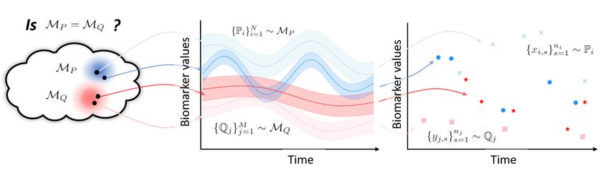
served example or set. See Figure 1 for an illustration of
Hypothesis tests are used to answer questions about a spe- this interpretation for the two sample problem. This set-up
cific dependency structure in data (e.g. independence be- is common in regression problems where one seeks to learn
tween variables, equality of distributions between samples a mapping from distributions to associated labels, see e.g.
etc). They are used in applications across the sciences where [40, 41], but is unexplored in hypothesis testing.
they serve as an essential tool to summarize experimental The goal of this paper is to introduce kernel two-sample and
data and quantify the evidence for discoveries on the rela- kernel independence tests defined on set-valued examples.
tionship of variables of interest, see e.g. [23] for a general
introduction. As a consequence, a growing body of work is We will show that tests defined in this space appropriately
constantly revisiting established modelling assumptions to encode individual-level heterogeneity, are much more flexi-
allow for consistent testing in increasingly heterogeneous ble, do not require heuristic pre-processing of data, and are
data sources. Examples include non-parametric tests formu- found to be more powerful than alternatives. We propose an
lated as distances in Hilbert space, see e.g. [12, 11, 9, 47], approach applicable to any kernel-based test that includes,
Accepted for the 37th Conference on Uncertainty in Artificial Intelligence (UAI 2021).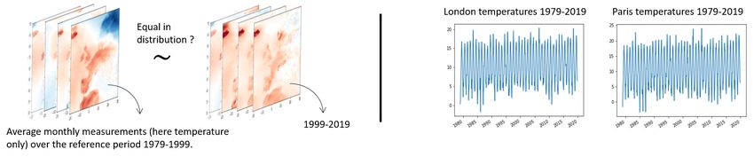
Figure 1: We consider an example from electronic health records to illustrate the proposed approach. Right panel: we observe irregular,
uncertain biomarker measurements over time in two groups of patients (treated and control) colored with different shades of red and blue,
the question being whether these populations have the same trajectory in distribution. Middle panel: we encode the uncertainty in each
patient trajectory by a probability distributions on the space of observations. Left panel: The two-sample problem is to test for equality in
distribution on the space of patient-specific distributions, rather than actual observations. This two-level hierarchy allows for noisy inputs
and irregular input sizes. A description of the notation and more details can be found in Section 3.1.

in addition to two-sample and independence tests described               Each {xi,j }nj=1
                                                                                        i
                                                                                            is a set of ni individual observations xi,j
here, conditional independence tests and three-variable in-              (typically in R ). We assume that {xi,j }nj=1
                                                                                          d                            i
                                                                                                                         are i.i.d sam-
teraction tests.                                                         ples from an unobserved probability distribution Pi . The
The technical challenge to achieve consistency of test deci-             probability distributions {Pi }N i=1 themselves have inherent
sions is that latent distributions on which tests are defined            variability, such as can be expected for example from dif-
are not available (and instead are approximated with each                ferent medical patients. We assume each one of them to
available set of observation). This introduces an additional             be drawn randomly from some unknown meta-distribution
layer of uncertainty that must be bounded to derive well-                MP defined over a set of probability measures P. We il-
defined asymptotic distributions for the proposed test statis-           lustrate this set-up in Figure 1 for the two-sample problem
tics. For this reason, we put emphasis also on the quality               (more details in Section 3.1).
of finite-dimensional approximations of the proposed tests,
with approaches to minimize test statistic variance and to               2.1   EMBEDDINGS OF DISTRIBUTIONS
tune hyperparameters for maximum power.
Our contributions are three-fold:                                        Let X be a measurable space of observations. We use a posi-
                                                                         tive definite bounded and measurable kernel k : X ×X → R
    1. We formally describe tests on set-valued data, and to             to represent distributions Pi on X , and independent sam-
       the best of our knowledge for the first time.                     ples {xi,j }nj=1
                                                                                       i
                                                                                          , as two functions µPi , and µ̂Pi respectively,
                                                                         called kernel mean embeddings [30]. Both are defined in the
    2. We demonstrate the consistency of these tests for the
                                                                         corresponding Reproducing Kernel Hilbert Space (RKHS)
       two-sample and independence testing problems.
                                                                         Hk by,
    3. We validate the proposed tests and optimization rou-                       Z
       tines on simulated experiments that show that one may                                                        1      X
                                                                         µPi :=       k(x, ·)dPi (x),     µ̂Pi :=                 k(x, ·).
       consistently discriminate between hypotheses on data                        X                                ni         ni
                                                                                                                         x∈{xi,j }j=1
       that was previously not amenable to hypothesis testing.
                                                                         To make inference on populations of distributions, the de-
                                                                         siratum however is on defining useful representations of
2     BACKGROUND
                                                                         distributions MP on the space probability measures, rather
                                                                         than on the space of observations. Christmann et al. [6]
The tests presented in this paper are formally defined on dis-
                                                                         showed that one may do so analogously to the definition
tributions. Testing on distributions is the problem of defining
                                                                         of kernels on X by treating mean embeddings µP them-
a test statistic that maps distributions to a scalar that quan-
                                                                         selves as inputs to kernel functions, µP replacing x ∈ X in
tifies the evidence for a hypothesis we might set on the
                                                                         the conventional learning setting as inputs to k, see eq. (2)
relationships in data. However, we do not have access to
                                                                         below.
probability distributions themselves, but rather distributions
are observed only through sets of samples,                               Accounting for variance in embedding approximations.
                                                                         In practice, each set representation µPi is limited to be ap-
                   {x1,j }nj=1
                            1
                               , ..., {xN,j }nj=1
                                               N
                                                  .             (1)      proximated by irregularly sampled observations {xi,j }nj=1i
                                                                                                                                     .
Not all mean embeddings µP are expected to provide the              as the Gaussian kernels, if used in both levels of the embed-
same amount of information about their underlying dis-              ding and defined on a compact metric space the resulting
tribution P. Indeed, the empirical mean embeddings µ̂Pi             embedding is injective (i.e. kernels are characteristic)1 .
                                                         √
converge to their population counterpart at a rate O(1/ ni )
                                                                    The empirical version of the RKHS distance, however, will
(see e.g. Lemma 1 in the Appendix and also [36]) in their set
                                                                    not necessarily be exactly zero even if the distributions
size ni . Rather than assuming access to a uniform sample of
                                                                    do coincide. Some variability is to be expected due to the
distributions {Pi }Ni=1 from MP , like we did with the raw          limited number of samples, and in contrast to conventional
observations {xi,j }nj=1
                       i
                         , we may account for this irregularity
                                                                    kernel tests, in the case considered here also due to the
and uncertainty in approximation by interpreting the set of
                                                                    variability in the estimation of set embeddings. Instead of
distributions as a weighted sample {(Pi , wi )}N i=1 ∼ MP .         testing on an i.i.d. sample {µPi }N   i=1 , we are testing over
Each weight quantifying the accuracy of the approximation
                                                                    the set {µ̂Pi }N
                                                                                   i=1 . There is an additional level of uncertainty
of each distribution with the limited samples available. The
                                                                    which must be accounted for.
corresponding population and empirical mean embedding
in this space may be written as,                                    In practice, tests are constructed such that a certain hypoth-
                                                                    esis is rejected whenever a test statistic exceeds a certain
                                             N
                                                                    threshold away from 0 [23]. Then, short from achieving
        Z                                    X
µM :=         K(µP , ·)dM(P),       µ̂M :=         wi K(µPi , ·).   perfect discrimination between two hypotheses, the goal of
          P                                  i=1
                                                                    hypothesis testing is to derive a threshold such that false
                                                             (2)
                                                                    positives are upper bounded by a design parameter α and
We will make use of the Gaussian kernel between distri-             false negatives are as low as possible.
butions defined K(µP , µQ ) := exp(−||µP − µQ ||2HK /2σ 2 )
[6, 29]. Note that for kernels on X , their RKHS consists of        2.3       RELATED WORK
functions X → R, while the kernel K lives on the space of
distributions on X , P(X ), and its RKHS consists of func-          Distances on sets. As a first observation, note that kernels
tions P(X ) → R. We may use K to learn from samples                 defined on sets directly, as done e.g. by [19], measuring the
that are individual distributions, rather than individual ob-       similarity between sets by the average pairwise point simi-
servations, as described in [6].                                    larities between the sets, are not known to be characteristic.
Relationships with learning on distributions. With this             Attempts have also been made to define kernels on the space
construction (i.e. kernels evaluated on mean embeddings)            of distributions, including probability product kernel [15],
[40] investigated generalization performance in distribu-           the Fisher kernel [14], diffusion kernels [20] and kernels
tional regression: regressing to a real-valued response from        arising from Kullback-Leibler divergences [28], none of
a probability distribution. Results that were subsequently ex-      them known to be characteristic and in this case with the
tended to study distributional regression for causal inference      shortcoming that many of the above are parameterized by a
in [26] and for transfer learning, see e.g. [5]. A technical        family of densities which may or may not hold in data.
contribution of this paper is to extend these results to demon-     Possible extensions to other tests. Deep learning has
strate consistent hypothesis testing on distributions.              emerged as an alternative for defining tests on structured
                                                                    objects. [27] define classifier two-sample tests and [24] use
2.2   HYPOTHESIS TESTING WITH KERNELS                               deep kernels to embed structured objects. Tests in these
                                                                    cases, however, are defined directly on the space of obser-
The advantage for hypothesis testing of mapping distribu-           vations, it is not clear how to input examples of varying
tions M and M0 to functions in an RKHS is that we may               sizes, or how to account for the uncertainty in individual
now say that M and M0 are close if the RKHS distance                observations especially if these change across sets.
||µM − µM0 ||HK is small [9]. This distance depends on              Other connections with hypothesis testing. Accommodat-
the choice of the kernel K and k; a crucial property of the         ing for input uncertainty has connections with robust hy-
embeddings is that for certain kernels the feature map is           pothesis testing. These tests attempt to explicitly enforce
injective. These kernels are called characteristic [37]. Prob-      invariances in test statistics in a certain uncertainty ball to
ability distributions may be distinguished exactly by their         remove irrelevant sources of variation [8, 13]. Other types
images in the RKHS, and also ||µM − µM0 ||HK is zero if             of invariances can also be enforced, for instance [21] use
and only if the distributions coincide [9]. From the statistical    features designed to be invariant to additive noise and use
testing point of view, this coincidence axiom is key as it          distances between those representations for hypothesis test-
ensures consistency of comparisons for any pair of different        ing. One may also use a model-based approach to capture
distributions.                                                            1
                                                                         Theorem 2.2 [6] technically shows that such kernels are uni-
As a key property of the set-up we have introduced, in Theo-        versal, but universal kernels on a compact metric space are known
rem 2.2 [6] demonstrated that for well known kernels, such          to be characteristic, see e.g. Theorem 1 [9].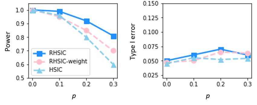
this uncertainty, for instance [4] use Gaussian processes and       follows [9],
compare posterior distributions. More generally, tests in the
functional data analysis literature, such as [46, 31, 44, 35, 7],     MMD2 :=EP,P0 ∼MP K(P, P0 ) + EQ,Q0 ∼MQ K(Q, Q0 )
may be consistently applied on regularly sampled time series                        − 2EP∼MP ,Q∼MQ K(P, Q)                             (4)
data with a strong time-dependence. The set representation
in (1) assumes instead each observation (and time stamp
                                                                    where K is the kernel on distributions given after equation
in the case of time series) to be drawn independently, a                                2
formalism that may be adequate for some problems (e.g.              (2). We denote M
                                                                                   \ MD the empirical estimator of the MMD2
sufficiently sparse and irregular time series as observed in        with expectations replaced by averages, obtained from in-
primary care electronic health records see e.g. [2, 1, 22]          dependent samples {Pi }N                        M
                                                                                             i=1 ∼ MP and {Qj }j=1 ∼ MQ .
and other set-valued data) but not others (e.g. frequently          The proposed statistic is defined by considering approxi-
sampled time series).                                               mate mean embeddings of each distribution and considering
                                                                    the weighted sample of their meta-distribution each of them
                                                                    represents,
3     HYPOTHESIS TESTS ON SETS
                                                                                     N
                                                                               2     X
                                                                     \ :=
                                                                    RMMD                    wPi wPj K(µ̂Pi , µ̂Pj )+
In the following sections, we propose tests to evaluate two
                                                                                    i,j=1
common hypotheses: the two sample problem of testing
                                                                     M                                     N,M
equality of distributions in two samples, and the indepen-           X                                     X
dence problem of testing whether joint distributions in                      wQi wQj K(µ̂Qi , µ̂Qj ) − 2           wPi wQj K(µ̂Pi , µ̂Qj )
                                                                     i,j=1                                 i,j=1
paired samples coincide with the product of their marginals.
For both tests, the exposition mirrors well-known results in        R stands for robust. Assume for now that all weights are
kernel hypothesis testing which we will only briefly describe       fixed wPi = 1/N, wQj = 1/M for all i, j. We return to the
(see [9, 12] for more background). The contribution of this         specification of weights in section 3.3. The asymptotic be-
paper is to show that tests defined with a second level of                            2
                                                                    haviour of M\ MD is well understood [9] and the test itself
sampling are consistent and to show that correctly weighting        is extensively used in many applications [25, 33]. However,
representations according to their set size is most efficient.      these results do not extend trivially if each independent set
Algorithm. We may summarize hypothesis testing in this              exhibits an additional source of variation due to the estima-
context as follows:                                                 tion of the mean embedding. In the following proposition,
                                                                    we bound the contribution of this additional source of varia-
    1. Embed the distributions {Pi }Ni=1 into an RKHS us-           tion and show that under the asymptotic regime where both
       ing approximations of the mean embeddings {µ̂Pi }N
                                                        i=1         the set sizes and number of sets grow larger, asymptotic
       computed with independent samples {xi,j }nj=1
                                                  i
                                                     ∼ Pi .         distributions are well defined.
    2. Define test statistics on this feature representations to    Proposition 1 (Asymptotic distribution). Let two samples
       test for a certain hypothesis or dependency structure in     of data be defined as above and let K be characteristic
       M.                                                           and LK -Lipschitz continuous. Then, under the null and
                                                                    alternative and in the regime of increasing set size ni and
                                                                    increasing sample size n, the asymptotic distributions of
                                                                           2                              2
3.1    THE TWO SAMPLE PROBLEM                                       RMMD
                                                                     \ coincides with that of M    \  MD .
                                                                    Proof. All proofs are given in the Appendix.
Consider a first collection of sets of observations, each i-
th set denoted {xi,s }ns=1
                        i
                            ∼ Pi , for a total of N such sets       In other words, the additional variability due to a second
with distributions {Pi }N i=1 ∼ MP , and define similarly a         level of sampling converges to 0 asymptotically, and thus the
                                                   nj
second collection of sets, each j-th set {yj,s }s=1    ∼ Qj ,       asymptotic distribution coverges to that of the well known
for {Qj }M
         j=1 ∼ MQ . The problem we consider is to test              MMD two sample test of [9].
whether,

      H0 : MP = MQ         or else   H1 : MP 6= MQ           (3)    3.2   THE INDEPENDENCE PROBLEM

holds on the basis of the observations available in each            Independence tests are concerned with the question of
set. We illustrate this problem in Figure 1. The proposed           whether two random variables are distributed independently
test statistic approximates the square of the RKHS distance         of each other. For this problem, we start with a collection of
between densities MP and MQ , also called Maximum                   paired distributions {(Pi , Qi )}N
                                                                                                     i=1 drawn from a joint dis-
Mean Discrepancy (MMD), which may be decomposed as                  tribution we denote MP Q , and denote their marginals MP
and MQ . The hypothesis problem is to determine whether, Proposition 2 (Asymptotic distribution). Let two samples
of data be defined as above and let K be characteristic
H0 : MP Q = MP MQ or else and LK -Lipschitz continuous. Then, under the null and
H1 : MP Q 6= MP MQ (5) alternative and in the regime of increasing set size ni and
increasing sample size n, the asymptotic distributions of
\ coincides with that of HSIC.
RHSIC [
Example. Consider an example from healthcare to illustrate
this problem. [ has been studied in
Independence testing with the HSIC
[12, 47, 16].
• A similar set-up as that given in Figure 1 may
be used to illustrate independence testing with set-
valued data. A common problem is identify de- 3.3 PRACTICAL REMARKS
pendencies between biomarkers, often observed ir-
regularly over time in many patients. For instance We make a number of remarks on the practical application
cholesterol levels {xi,t1 , . . . , xi,tni } and blood pres- of our tests.
sure {yi,t1 , . . . , yi,tni } may be observed over times
t1 , . . . , tni in N individuals i = 1, . . . , N . To formally • Weights for high power. Set sizes in practice may be
test for dependencies between these samples one must limited. In the asymptotic regime of increasing number of
account for the irregularity in observation time and sets but finite set size, the properties of the estimator may
uncertainty in biomarker reads. This can be done by depend on appropriately weighting sets for high power.
considering instead distributions Pi and Qi and testing The proposed weighting scheme addresses this point.
for independence in this space directly. Recall that each individual observation xij is drawn inde-
pendently from their respective distributions Pi . Other fac-
As in the two-sample test, we may quantify the difference tors of variations assumed to be common across sets, the
between distributions using the RKHS distance ||µMP Q − variance of the approximate embedding µ̂Pi is therefore
µMP ⊗µMQ ||2HS . Kernels K, L are assumed characteristic; proportional to 1/ni (i.e. the variation in approximation
|| · ||HS is the norm on the space of HK → HL Hilbert- of mean embeddings is due solely to diverging set sizes).
Schmidt operators, and ⊗ denotes the tensor product, such When mean embeddings have different variances, it is
that (a ⊗ b)c = ahb, ci for a, b, c elements of a Hilbert space. efficient to give less weight to mean embeddings that have
This distance is called the Hilbert Schmidt Independence high variances. By efficient in this context, we mean high-
Criterion (HSIC) [10, 12]. est asymptotic power of tests based on mean embedding
representations of sets.
Two empirical estimators can be written: one assuming ac-
cess to independent samples MP Q and one with indepen- For V -statistics the asymptotic power function is well
dent samples from each of the paired distributions sampled known, and an argument involving the delta method for
from MP Q , differentiable kernels, expanded on in the Appendix, can
be used to determine
P the optimal weights to be given by
[ = Tr (KHLH)/N 2
HSIC wPi := ni / i ni for each i.
\ = Tr (K̂H L̂H) · N 2 • Hyperparameters for high power. With a similar intu-
RHSIC (6)
ition, even though in theory we can expect high power for
for kernel matrices with (i, j) entries Kij = K(Pi , Pj ) = any alternative hypothesis and any choice of kernel, with
hµPi , µPj iHK and Lij = hµQi , µQj iHL for the popula- finite sample size, some kernel hyperparameters will give
higher power than others. The proposed tests optimize
tion version and K̂ij = wPi wPj hµ̂Pi , µ̂Pj iHK and L̂ij =
the choice of kernels by choosing hyperparameters that
wQi wQj hµ̂Qi , µ̂Qj iHL with mean embeddings replaced by
minimize the asymptotic variance under the alternative
their weighted finite sample counterparts for the robust
similarly to [39, 16]. But, in addition, we extend the opti-
alternative. Assume for now that all weights are fixed
mization to tune both the mean embedding to represent
wPi = 1/N, wQj = 1/M for all i, j. The centering matrix
sets and the kernel used for comparisons in Hilbert space.
is defined by H = I − N1 11T and Tr is the trace operator. Please find more details in the Appendix.
Here, similarly to the two sample problem, approximations • Low-dimensional approximations for large scale data.
due to a second level of sampling are well behaved and mir- Testing on distributions as described is often not scalable
ror those of the robust statistic for the two-sample problem. for even to large datasets, as computing each of the entries
In particular, that asymptotic distributions of the RHSIC of the relevant kernel matrices requires defining a high-
and the HSIC coincide in the regime with increasing set dimensional mean embedding. To define test statistics on
size and increasing sample size, making hypothesis testing these representations we further embed the non-linear fea-
\ consistent for the independence problem in
with the RHSIC ture space Hk defined by k into a random low dimensional
equation (5). Euclidean space using their expansion in Hilbert space asa linear combination of the Fourier basis as proposed by • For the independence problem we consider: the HSIC
[34, 32]. If we draw m samples from the Gaussian spec- [12], the Randomized Dependence Coefficient (RDC)
tral measure, we can approximate the Gaussian kernel k [26] and Pearson Correlation Coefficient (PCC).
by,
m
For all kernel-based tests, because their null distributions
2 X are given by an infinite sum of weighted χ2 variables (no
k(x, y) ≈ cos(hωj , xi + bj ) cos(hωj , yi + bj )
m j=1 closed-form quantiles), in each trial we use 400 random
permutations to approximate the null distribution. We give
= hφ(x), φ(y)i more details on the implementation of each of these tests in
the Appendix.
1 , ..., ωm ∼ N (0, γ), b1 , ..., bm ∼ U[0, 2π], and
where ωq
2
φ(x) = m [cos(ω1 x + b1 ), ..., cos(ωm x + bm )] ∈ Rm
[32]. The mean embedding µP = EX∼P φ(X) can then be
4.1 TWO-SAMPLE PROBLEM
approximated with elements in the span of (cos(hωj , xi +
bj ))m
j=1 . By averaging over the available ni samples
in Xi from the distribution Pi , the approximate finite- Experiment design. Each one of the two samples is de-
dimensional embedding is given by, fined by a family of N distributions {Pi }N
i=1 we take to be
Gaussian Pi = η sin(2πt) + N (0, σi + σ). The variabil-
1 X
r
2 ity between the {Pi }N
i=1 is specified by σi , drawn from a
µ̂Pi ,m = (cos(hwj , xi + bj ))m
j=1 ∈ R
m
one-parameter inverse gamma distribution, which mimics
ni m
ni
x∈{xij }j=1 the behaviour of the meta-distribution and the observation
pattern we may observe in heterogeneous data. The differ-
All implementation details, including the above approxima- ence between two populations of sampled distributions is
tions, are given in the Appendix. the mean amplitude η and/or shifts in baseline variance σ.
Two-sample problems become harder whenever these pa-
rameters converge to the same value in the two samples
4 SYNTHETIC DATA EXPERIMENTS and are easier when they diverge. The sampled Gaussian
distributions themselves are not observable and, in turn, we
The purpose of synthetic experiments will be to test power: have access to observations xij ∼ Pi . Each xij is obtained
the rate at which we correctly reject H0 when it is false, as by fixing t to tj ∼ U[0, 1] and subsequently sampling from
we increase the difficulty of the testing problems; and Type the Gaussian.
I error: the rate at which we incorrectly reject H0 when it
is true. The result is two collections of noisy time series with non-
linear dynamics. Each time series, or set of observations, is
In all experiments, α (the target Type I error) is set to 0.05, irregularly sampled with noise levels that vary between sets.
the number of time series is set to N = 500, the number of
observations made on each time series is random between 5 Results. We report performance for the two sample prob-
and 50, and each problem is repeated for 500 trials. lems in the top row of Figure 2. Power is measured in three
experiments: first, as we increase the difference in time se-
Tests for empirical comparisons. To the best of our knowl- ries amplitude (with equal variance σ = 0.1), second as
edge, no existing test naturally accommodates for set-valued we increase the observation variance (with equal amplitude
data with irregular sizes. Our approach to empirical com- η = 1) between the two populations, and third as the dimen-
parisons will be to coerce the data into a fixed dimensional sion of each time series increases (on data sampled with a
vector in a well-defined manner, and evaluate existing tests single dimension with a difference in amplitude equal to
on this representation. To do so, we focus on time-series 0.25 and other dimensions with no difference). Type I error
-like data which we interpolate along the time axis with is shown as a function of the number of samples.
cubic splines and evaluate at a fixed number of time points.
All tests approximately control for type I error at the desired
• The following tests are evaluated for the two-sample prob- threshold. In terms of power, we observe the RMMD to out-
lem. The MMD [9] with hyperparameters optimized for perform across all experiments with an important contrast on
maximum power, two-sample classifier tests [27] which the difference in performance with the MMD. Even though
involve fitting a deep classifier. We considered a recurrent using similar test statistics, the RMMD much more faithfully
neural network with GRU cells for sequential data (C2ST- captures the irregularity and uncertainty of every individual
GRU) and the DeepSets approach of [45] modelling set of observations. RMMD similarly outperforms C2ST-
permutation invariance to be expected in sets (C2ST- based tests, the strongest baselines, with up to a two-fold
Sets). We consider also the Gaussian process-based test increase in power for small differences in amplitude and
(GP2ST) by [4]. variance.Figure 2: Power (higher better) and Type I error (at level 0.05) on synthetic data. The rightmost panel gives type I error with approximate
control at the level α = 0.05 for all methods. Top row: two-sample problem. Bottom row: independence problem. RMMD and RHSIC
are the proposed tests.
4.2 INDEPENDENCE PROBLEM resentations as none of them avoids interpolating between
observations before testing independence which we hypoth-
esize is one reason for their underperformance. This is con-
Experiment design. We aim to construct pairs of distri- sistent with the increasing variance experiment, in this case
butions (Pi , Qi ). Define the mean of each distribution Pi increasing variance worsens interpolation performance.
as fi (t) := βi sin(2πt) + αi t. Differently than in the two-
sample problem, the variability among the {Pi } appears in
the amplitude and trend of the sine function, let these be
βi ∼ U[0.5, 1.5] and αi ∼ U[−0.5, 0.5]. Once these param-
eters are sampled, paired distributions (Pi , Qi ) are given
by Pi = fi (t) + N (0, σ) and Qi = g(fi (t)) + N (0, σ).
Each observation from this pair is obtained as in the two
sample problem by fixing a random t and sampling from 5 TESTING ON LUNG FUNCTION DATA
the resulting distribution.
OF CYSTIC FIBROSIS PATIENTS
The difficulty of the problem is governed by two factors: g
and σ. g determines the dependency between the two func-
tions. In every trial, g(x) is randomly chosen from the set For people with Cystic Fibrosis (CF), mucus in the lungs
of functions {x2 , x3 , cos(x), exp(−x)}. Testing for depen- is linked with chronic infections that can cause permanent
dency is hard also for increasing variance σ of observations, damage, making it harder to breathe [17]. This condition
as this makes the dependent paired samples appear inde- is often measured over time using FEV1% predicted;
pendent. A sample of dependent sets of data using this data the Forced Expiratory Volume of air in the first second of a
generating mechanism is given in the lower rightmost panel forced exhaled breath we would expect for a person without
of Figure 2. CF of the same age, gender, height, and ethnicity [42]. For
example, a person with CF who has FEV1% predicted
Results. Power and type I error are shown in the bottom row
equal to 50% can breathe out half the amount of air as we
of Figure . The bottom row of Figure 2 gives performance re-
would expect from a comparable person without CF. In this
sults for the independence problem. In the first two leftmost
experiment, we work with data from the UK Cystic Fibrosis
panels we evaluate power as we increase the variance of
Trust containing records from 10, 980 patients with approx-
paired time series and as we increase the dimensionality of
imately annual follow ups between 2008 and 2015, with the
each observation for a fixed variance σ = 0.5. The bottom
objective of better understanding the dependence of lung
rightmost plot shows a sample of two dependent noisy time
function over time with other biomarkers. For this problem
series, colored blue and red respectively, for illustration.
we found a significant influence of Body Mass Index (BMI)
The conclusions for this problem mirror the two-sample over time and the number of days under intravenous antibi-
testing experiments, with however a much larger increase otics in a given year; both already known to be associated
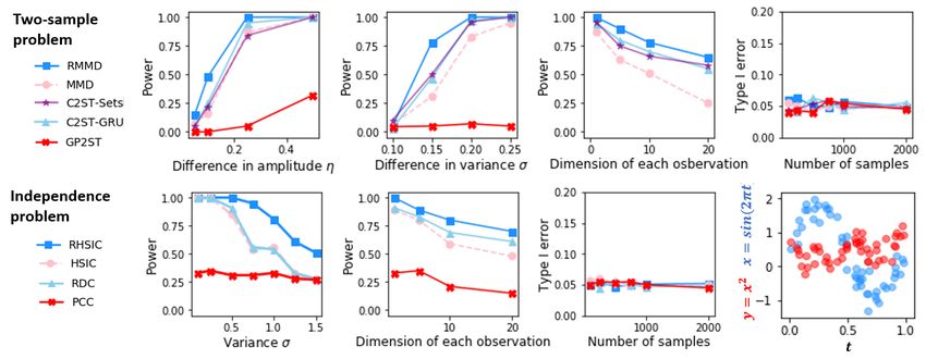
in power over alternatives, all using less flexible data rep- with lung function [43, 18].Figure 3: Illustration of the two-sample problem with global set-valued data versus local time series data.
globe at a given time as a set of data points. Each set sam-
pled from a probability distribution that represents the global
weather pattern of the climate. We follow standard descrip-
tions to define the climate as a collection of these sets ob-
served over a period of 20 years. The problem is to test
for significant differences in climate, represented by the
evolution of bags of (multi-channel) images, over time (see
Figure 3).
Figure 4: Power and Type I error on Cystic Fibrosis data.
Experiment design. The data is publicly available, pro-
vided by the Copernicus Climate Change Service2 . We in-
We use this information to create a set of problems under the clude a total of 12 climate variables identified as essential
alternative H1 with an additional twist. We increase hetero- to characterize the climate3 , including temperature, atmo-
geneity among patients by artificially removing a proportion spheric pressure, observed over monthly periods for the
p of densely sampled patients (here more than 4 record- last 40 years across Europe. The available data thus con-
ings). The problem is to test for independence between a sists of a two streams of sets {xi,j }nj=1
i
and {yi,j }nj=1
i
for
patients two-dimensional trajectory of BMI and antibiotics i = 1, . . . , 144 (12 months over 20 years). The first de-
measurements over time, and their lung function trajectory scribes the climate over the period 1979 − 1999, and the
over time. In this set-up, we expect the information content second set over the period 1999 − 2019. Both contain mea-
of the average patient to decrease, a scenario that lends it- surements xi,j ∈ R12 (yi,j respectively) in approximately
self to an importance-weighted approach (more weight on ni = 250 different locations (approximately because not all
densely sampled trajectories), such as described in section locations are consistently observed over time) which makes
3.3. In this section we test this property, which we found ad- the length of each set irregular. Existing tests would thus
vantageous for higher missingness data patterns, as shown require some form of interpolation which is not trivial over
in Figure 4. In this case, power tends to be higher after space and time in this case.
weighting (RHSIC) versus not weighting (RHSIC-weight). Problem. The problem is to test for the hypothesis of
We report also type I errors, well controlled by all methods, equally distributed climate data over the past 4 decades.
evaluated after shuffling the lung function trajectories be- We conduct 5 different tests: on data from the European,
tween patients, such as to break the associations between African, North American, South American and South-East
BMI and antibiotics, and lung function trajectories. Asian regions.
Results. RMMD rejects the hypothesis of equally dis-
6 TESTING ON CLIMATE DATA tributed climate data over the past 4 decades in Europe
(p-value 0.0002), Africa (p-value 0.0014), and South Amer-
This experiment explores the use of extensive weather data ica (p-value 0.0001) but fails to reject at a level of 0.01
to determine whether the recent rapid changes in climate for North America (p-value 0.016) and South-East Asia
associated with human-induced activities significantly differ (p-value 0.036).
from natural climate variability. A number of variables are In the case of Europe, we note that this result would be
used to monitor the state of the climate including precipi- different if only a particular location was considered (which
tation, wind patterns, and atmospheric composition among could have been a viable reductionist strategy to use existing
others. It depends on the latitude and longitude, and regions tests). For instance, we found that the RMMD applied to
may vary and evolve differently over time [38]. 2
https://climate.copernicus.eu/.
Interpretation as set-valued data. We can think of the 3
https://public.wmo.int/en/programmes/global-climate-
multivariate measurements in different locations across the observing-system/essential-climate-variablesclimate data over the same periods in London and Paris to [6] Andreas Christmann and Ingo Steinwart. Universal
not be significantly different (p-value 0.21). See Figure 3 kernels on non-standard input spaces. In Advances
for the time series of Paris and London temperature data. in neural information processing systems, pages 406–
This experiment demonstrates the potential benefits of using 414, 2010.
more flexible tests that better represent available data to
[7] Livio Corain, Viatcheslav B Melas, Andrey Pepely-
faithfully investigate complex phenomena such as climate
shev, and Luigi Salmaso. New insights on permu-
that involve multiple measurements over time and space.
tation approach for hypothesis testing on functional
data. Advances in Data Analysis and Classification,
7 CONCLUSIONS 8(3):339–356, 2014.
[8] Rui Gao, Liyan Xie, Yao Xie, and Huan Xu. Robust
In this paper we extended the toolkit of applied statisticians hypothesis testing using wasserstein uncertainty sets.
to do hypothesis testing on set-valued data. We have shown In Advances in Neural Information Processing Sys-
that by appropriately representing each set of observations tems, pages 7902–7912, 2018.
in a Hilbert space, kernel-based hypothesis testing may be
applied consistently. Specifically, we introduced tests for [9] Arthur Gretton, Karsten M Borgwardt, Malte J Rasch,
the two-sample and the independence problem, derived their Bernhard Schölkopf, and Alexander Smola. A ker-
asymptotic distributions and provided efficient algorithms nel two-sample test. Journal of Machine Learning
and optimization schemes to analyse a wide range of scenar- Research, 13(Mar):723–773, 2012.
ios in an automatic fashion.
[10] Arthur Gretton, Olivier Bousquet, Alex Smola, and
Bernhard Schölkopf. Measuring statistical dependence
8 ACKNOWLEDGEMENTS with hilbert-schmidt norms. In International confer-
ence on algorithmic learning theory, pages 63–77.
We thank the anonymous reviewers for valuable feedback Springer, 2005.
and the UK Cystic Fibrosis Trust for access to data. All pa- [11] Arthur Gretton, Kenji Fukumizu, Zaid Harchaoui, and
tient data was deidentified. This work was supported by the Bharath K Sriperumbudur. A fast, consistent kernel
Alan Turing Institute under the EPSRC grant EP/N510129/1, two-sample test. In Advances in neural information
the ONR and the NSF grants number 1462245 and number processing systems, pages 673–681, 2009.
1533983.
[12] Arthur Gretton, Kenji Fukumizu, Choon H Teo,
Le Song, Bernhard Schölkopf, and Alex J Smola. A
REFERENCES kernel statistical test of independence. In Advances
in neural information processing systems, pages 585–
[1] Ahmed Alaa and Mihaela van der Schaar. Atten- 592, 2008.
tive state-space modeling of disease progression. In
Advances in neural information processing systems, [13] Gökhan Gül and Abdelhak M Zoubir. Robust hypothe-
2019. sis testing with \α-divergence. IEEE Transactions on
Signal Processing, 64(18):4737–4750, 2016.
[2] Alexis Bellot and Mihaela Van Der Schaar. Flexible
[14] Tommi Jaakkola and David Haussler. Exploiting gener-
modelling of longitudinal medical data: A bayesian
ative models in discriminative classifiers. In Advances
nonparametric approach. ACM Transactions on Com-
in neural information processing systems, pages 487–
puting for Healthcare, 1(1):1–15, 2020.
493, 1999.
[3] Alexis Bellot and Mihaela van der Schaar. Conditional [15] Tony Jebara, Risi Kondor, and Andrew Howard. Prob-
independence testing using generative adversarial net- ability product kernels. Journal of Machine Learning
works. In Advances in Neural Information Processing Research, 5(Jul):819–844, 2004.
Systems, pages 2202–2211, 2019.
[16] Wittawat Jitkrittum, Zoltén Szabó, and Arthur Gretton.
[4] Alessio Benavoli and Francesca Mangili. Gaussian An adaptive test of independence with analytic kernel
processes for bayesian hypothesis tests on regression embeddings. In Proceedings of the 34th International
functions. In Artificial intelligence and statistics, pages Conference on Machine Learning-Volume 70, pages
74–82, 2015. 1742–1751. JMLR. org, 2017.
[5] Gilles Blanchard, Aniket Anand Deshmukh, Urun Do- [17] Eitan Kerem, Joseph Reisman, Mary Corey, Gerard J
gan, Gyemin Lee, and Clayton Scott. Domain general- Canny, and Henry Levison. Prediction of mortality in
ization by marginal transfer learning. arXiv preprint patients with cystic fibrosis. New England Journal of
arXiv:1711.07910, 2017. Medicine, 326(18):1187–1191, 1992.[18] Eitan Kerem, Laura Viviani, Anna Zolin, Stephanie [30] Krikamol Muandet, Kenji Fukumizu, Bharath Sripe-
MacNeill, Elpis Hatziagorou, Helmut Ellemunter, rumbudur, and Bernhard Schölkopf. Kernel mean em-
Pavel Drevinek, Vincent Gulmans, Uros Krivec, and bedding of distributions: A review and beyond. arXiv
Hanne Olesen. Factors associated with fev1 decline preprint arXiv:1605.09522, 2016.
in cystic fibrosis: analysis of the ecfs patient registry.
European Respiratory Journal, 43(1):125–133, 2014. [31] Victor M Panaretos, David Kraus, and John H Mad-
docks. Second-order comparison of gaussian random
[19] Risi Kondor and Tony Jebara. A kernel between sets functions and the geometry of dna minicircles. Journal
of vectors. In Proceedings of the 20th International of the American Statistical Association, 105(490):670–
Conference on Machine Learning (ICML-03), pages 682, 2010.
361–368, 2003.
[32] Ali Rahimi and Benjamin Recht. Random features
[20] John Lafferty and Guy Lebanon. Diffusion kernels for large-scale kernel machines. In Advances in neu-
on statistical manifolds. Journal of Machine Learning ral information processing systems, pages 1177–1184,
Research, 6(Jan):129–163, 2005. 2008.
[21] Ho Chung Law, Christopher Yau, and Dino Sejdinovic.
[33] Anant Raj, Ho Chung Leon Law, Dino Sejdinovic,
Testing and learning on distributions with symmetric
and Mijung Park. A differentially private kernel two-
noise invariance. In Advances in Neural Information
sample test. In Joint European Conference on Machine
Processing Systems, pages 1343–1353, 2017.
Learning and Knowledge Discovery in Databases,
[22] Changhee Lee and Mihaela Van Der Schaar. Tempo- pages 697–724. Springer, 2019.
ral phenotyping using deep predictive clustering of
disease progression. In International Conference on [34] Walter Rudin. Fourier analysis on groups, volume
Machine Learning, pages 5767–5777. PMLR, 2020. 121967. Wiley Online Library, 1962.
[23] Erich L Lehmann and Joseph P Romano. Testing [35] Łukasz Smaga and Jin-Ting Zhang. Linear hypothesis
statistical hypotheses. Springer Science & Business testing with functional data. Technometrics, 61(1):99–
Media, 2006. 110, 2019.
[24] Feng Liu, Wenkai Xu, Jie Lu, Guangquan Zhang, [36] Bharath K Sriperumbudur, Kenji Fukumizu, Arthur
Arthur Gretton, and DJ Sutherland. Learning deep Gretton, Bernhard Schölkopf, Gert RG Lanckriet, et al.
kernels for non-parametric two-sample tests. arXiv On the empirical estimation of integral probability
preprint arXiv:2002.09116, 2020. metrics. Electronic Journal of Statistics, 6:1550–1599,
2012.
[25] James R Lloyd and Zoubin Ghahramani. Statistical
model criticism using kernel two sample tests. In [37] Bharath K Sriperumbudur, Kenji Fukumizu, and
Advances in Neural Information Processing Systems, Gert RG Lanckriet. Universality, characteristic kernels
pages 829–837, 2015. and rkhs embedding of measures. Journal of Machine
[26] David Lopez-Paz, Philipp Hennig, and Bernhard Learning Research, 12(Jul):2389–2410, 2011.
Schölkopf. The randomized dependence coefficient.
[38] Thomas Stocker. Introduction to climate modelling.
In Advances in neural information processing systems,
Springer Science & Business Media, 2011.
pages 1–9, 2013.
[27] David Lopez-Paz and Maxime Oquab. Revisiting clas- [39] Dougal J Sutherland, Hsiao-Yu Tung, Heiko Strath-
sifier two-sample tests. In International Conference mann, Soumyajit De, Aaditya Ramdas, Alex Smola,
on Learning Representations, 2016. and Arthur Gretton. Generative models and model
criticism via optimized maximum mean discrepancy.
[28] Pedro J Moreno, Purdy P Ho, and Nuno Vasconcelos. arXiv preprint arXiv:1611.04488, 2016.
A kullback-leibler divergence based kernel for svm
classification in multimedia applications. In Advances [40] Zoltán Szabó, Arthur Gretton, Barnabás Póczos, and
in neural information processing systems, pages 1385– Bharath Sriperumbudur. Two-stage sampled learning
1392, 2004. theory on distributions. In Artificial Intelligence and
Statistics, pages 948–957, 2015.
[29] Krikamol Muandet, Kenji Fukumizu, Francesco Din-
uzzo, and Bernhard Schölkopf. Learning from distri- [41] Zoltán Szabó, Bharath K Sriperumbudur, Barnabás
butions via support measure machines. In Advances in Póczos, and Arthur Gretton. Learning theory for distri-
neural information processing systems, pages 10–18, bution regression. The Journal of Machine Learning
2012. Research, 17(1):5272–5311, 2016.[42] David Taylor-Robinson, Margaret Whitehead, Finn
Diderichsen, Hanne Vebert Olesen, Tania Pressler,
Rosalind L Smyth, and Peter Diggle. Understand-
ing the natural progression in% fev1 decline in pa-
tients with cystic fibrosis: a longitudinal study. Thorax,
67(10):860–866, 2012.
[43] Jeffrey S Wagener, Michael J Williams, Stefanie J Mil-
lar, Wayne J Morgan, David J Pasta, and Michael W
Konstan. Pulmonary exacerbations and acute declines
in lung function in patients with cystic fibrosis. Jour-
nal of Cystic Fibrosis, 17(4):496–502, 2018.
[44] George Wynne and Andrew B Duncan. A kernel
two-sample test for functional data. arXiv preprint
arXiv:2008.11095, 2020.
[45] Manzil Zaheer, Satwik Kottur, Siamak Ravanbakhsh,
Barnabas Poczos, Russ R Salakhutdinov, and Alexan-
der J Smola. Deep sets. In Advances in neural infor-
mation processing systems, pages 3391–3401, 2017.
[46] Jin-Ting Zhang. Statistical inferences for linear models
with functional responses. Statistica Sinica, pages
1431–1451, 2011.
[47] Qinyi Zhang, Sarah Filippi, Arthur Gretton, and Dino
Sejdinovic. Large-scale kernel methods for indepen-
dence testing. Statistics and Computing, 28(1):113–
130, 2018.You can also read