ATTRICI v1.1 - counterfactual climate for impact attribution
←
→
Page content transcription
If your browser does not render page correctly, please read the page content below
Geosci. Model Dev., 14, 5269–5284, 2021
https://doi.org/10.5194/gmd-14-5269-2021
© Author(s) 2021. This work is distributed under
the Creative Commons Attribution 4.0 License.

ATTRICI v1.1 – counterfactual climate for impact attribution
Matthias Mengel, Simon Treu, Stefan Lange, and Katja Frieler
Potsdam Institute for Climate Impact Research (PIK), Member of the Leibniz Association,
P.O. Box 60 12 03, 14412 Potsdam, Germany

Correspondence: Matthias Mengel (matthias.mengel@pik-potsdam.de)

Received: 15 May 2020 – Discussion started: 30 June 2020
Revised: 29 June 2021 – Accepted: 29 June 2021 – Published: 20 August 2021

Abstract. Attribution in its general definition aims to quan-     the observed trend in climate to the magnitude of individ-
tify drivers of change in a system. According to IPCC Work-       ual impact events. Attribution of climate impacts to anthro-
ing Group II (WGII) a change in a natural, human or man-          pogenic forcing would need an additional step separating an-
aged system is attributed to climate change by quantifying        thropogenic climate forcing from other sources of climate
the difference between the observed state of the system and       trends, which is not covered by our method.
a counterfactual baseline that characterizes the system’s be-
havior in the absence of climate change, where “climate
change refers to any long-term trend in climate, irrespec-
tive of its cause” (IPCC, 2014). Impact attribution following     1   Introduction
this definition remains a challenge because the counterfac-
tual baseline, which characterizes the system behavior in the     Global mean temperature (GMT) has recently surpassed 1 ◦ C
hypothetical absence of climate change, cannot be observed.       warming above pre-industrial levels (IPCC, 2018). The im-
Process-based and empirical impact models can fill this gap       pact of the realized change in climate has also started to be-
as they allow us to simulate the counterfactual climate im-       come detectable in natural, human or managed systems such
pact baseline. In those simulations, the models are forced by     as freshwater resources, terrestrial water systems, coastal
observed direct (human) drivers such as land use changes,         systems, oceans, food production systems, the economy,
changes in water or agricultural management but a counter-        human health, security and livelihoods (IPCC, 2014). The
factual climate without long-term changes. We here present        causal chain from climate change to climate impacts is of-
ATTRICI (ATTRIbuting Climate Impacts), an approach to             ten complex and intertwined with additional drivers, such as
construct the required counterfactual stationary climate data     changes in management that alter climate-induced changes
from observational (factual) climate data. Our method identi-     in crop yields (Butler et al., 2018; Iizumi et al., 2018; Zhu
fies the long-term shifts in the considered daily climate vari-   et al., 2019) and land use changes adding to climate-driven
ables that are correlated to global mean temperature change       changes in biodiversity (Hof et al., 2018).
assuming a smooth annual cycle of the associated scaling co-         Attribution in its most general definition aims to quantify
efficients for each day of the year. The produced counter-        the drivers of change in a system. The systems and drivers
factual climate datasets are used as forcing data within the      considered in attribution studies vary between disciplines. In
impact attribution setup of the Inter-Sectoral Impact Model       climate science, the “classical” attribution framework refers
Intercomparison Project (ISIMIP3a). Our method preserves          to the attribution of changes in the climate system to anthro-
the internal variability of the observed data in the sense that   pogenic forcing (Hegerl et al., 2010; WGI contribution to
factual and counterfactual data for a given day have the same     IPCC, 2013) (“climate attribution”; see first arrow in Fig. 1).
rank in their respective statistical distributions. The associ-   It addresses the following question: what is the contribution
ated impact model simulations allow for quantifying the con-      of anthropogenic emissions of greenhouse gases and aerosols
tribution of climate change to observed long-term changes         or land use changes to observed changes in climatic vari-
in impact indicators and for quantifying the contribution of      ables, most prominently temperature and precipitation? As
                                                                  the response of the climate system to these forcings is often

Published by Copernicus Publications on behalf of the European Geosciences Union.
5270                                                                                                M. Mengel et al.: ATTRICI v1.1

                                                                        change refers to any long-term trend in climate, irrespective
                                                                        of its cause” (IPCC, 2014, chap. 18.2.1).
                                                                           While in principle changes in natural, human and man-
                                                                        aged systems could also be attributed to anthropogenic cli-
                                                                        mate forcing (“impact attribution to anthropogenic climate
                                                                        forcing”, first and second arrow in Fig. 1, Pall et al., 2011;
                                                                        Schaller et al., 2016; Mitchell et al., 2016), we focus on “im-
                                                                        pact attribution to climate change” as described in the WGII
                                                                        definition and introduce a climate dataset that can be used
                                                                        as input to climate impact models to characterize the sys-
Figure 1. Differences between drivers and affected systems in attri-    tem’s behavior in the absence of climate change (second ar-
bution research. Climate attribution (first arrow) is a focus of IPCC   row in Fig. 1). The dataset is derived from the observed re-
WGI (IPCC, 2013), and (climate) impact attribution is a focus of        alization of climate, excluding the analysis how climate vari-
IPCC WGII (IPCC, 2014, chap. 18). The methodology and data
                                                                        ability could produce alternative realizations of factual or
presented here facilitate the use of (process-based) impact models
                                                                        counterfactual climate. The attribution approach is thus de-
to attribute observed changes in human, managed and natural sys-
tems to climate change (second arrow). The additional step of attri-    terministic and not probabilistic, focusing on the separation
bution to anthropogenic climate forcing (first and second arrow) is     of climate change from direct human influences as potential
not addressed here.                                                     drivers of changes in the impacted systems. Concerning the
                                                                        internal variability within impacted systems, impact models
                                                                        to date largely do not resolve such variability and model a de-
veiled by the chaotic nature of the climate system, climate at-         terministic response to external drivers. Our approach would
tribution usually builds on probabilistic approaches compar-            however allow for probabilistic attribution to climate change
ing an entire ensemble of climate model simulations includ-             once impact models resolve internal variability.
ing anthropogenic forcings against a counterfactual ensemble               The method proposed here is designed to generate a sta-
excluding these forcings as, e.g., generated within DAMIP               tionary climate without long-term changes. The statistical
(Gillett et al., 2016) to separate forced changes from inter-           model used to produce this counterfactual climate removes
nal variability. Climate attribution can refer to observed long-        the long-term change correlated with (but not necessarily
term trends (WGI contribution to IPCC, 2013, chap. 10) or               caused by) large-scale climate change, represented by GMT
individual events (Trenberth et al., 2015; NAS, 2016; Stott             change instead of a simple temporal trend (see Methods).
et al., 2016). Given the probabilistic setting, results are of-         The method preserves the internal variability of the observed
ten formulated as statements such as “anthropogenic climate             time series by additively (e.g., for temperature) or multiplica-
forcing has increased the probability of occurrence of the ob-          tively (e.g., for precipitation) removing a long-term trend,
served trend or the intensity or duration of a specific extreme         such that a particularly warm or dry day compared to the
event”. In a non-probabilistic framework the intensity of an            long-term trend remains a particularly warm or dry day in the
observed event can be attributed to the observed realization            counterfactual climate. In this regard, the approach is similar
of climate change by comparing the event magnitude in the               to the subtraction of a climate trend done by Diffenbaugh
observed time series to the magnitude of the same event in a            and Burke (2019) to attribute historical changes in economic
detrended version of the observed time series (quantification           growth or to attribute changes in land area burned by wild-
of the “contribution of the observed trend to event magni-              fires (Abatzoglou and Williams, 2016). However, while both
tude”, Diffenbaugh et al., 2017). This type of attribution to           studies subtract the anthropogenic warming derived from cli-
climate change does not address the reasons of the observed             mate model simulations, we subtract the realized long-term
climate trend.                                                          trend of the data irrespective of its cause (see WGII defini-
   In addition to climate attribution, research on impact attri-        tion).
bution addresses the following question: to what degree are                The stationary climate dataset can then be used as input
observed changes in natural, human and managed systems                  to climate impact models for impact attribution to climate
induced by observed changes in climate (Fig. 1, second ar-              change, as illustrated in Fig. 2. In a first step the climate im-
row)? In the Working Group II (WGII) contribution to the                pact model forced by observed climate and socio-economic
IPCC AR5, an entire chapter was dedicated to the topic in-              drivers has to demonstrate being able to reproduce the ob-
cluding the following definition: an impact of climate change           served changes in natural, human and managed systems as
is “detected” if the observed state of the system differs from          measured by an impact indicator (comparison of black and
a counterfactual baseline that characterizes the system’s be-           blue solid lines in Fig. 2). The attribution of the observed
havior in the absence of changes in climate (IPCC, 2014,                changes in natural, human and managed systems is built on
chap. 18.2.1), and “attribution” is the quantification of the           a high explanatory power of the factual simulations. Then, in
contribution of climate change to the observed change in the            a second step, that factual simulation can be compared to a
natural, human or managed system. In both cases “climate                counterfactual simulation, forced by counterfactual climate

Geosci. Model Dev., 14, 5269–5284, 2021                                                  https://doi.org/10.5194/gmd-14-5269-2021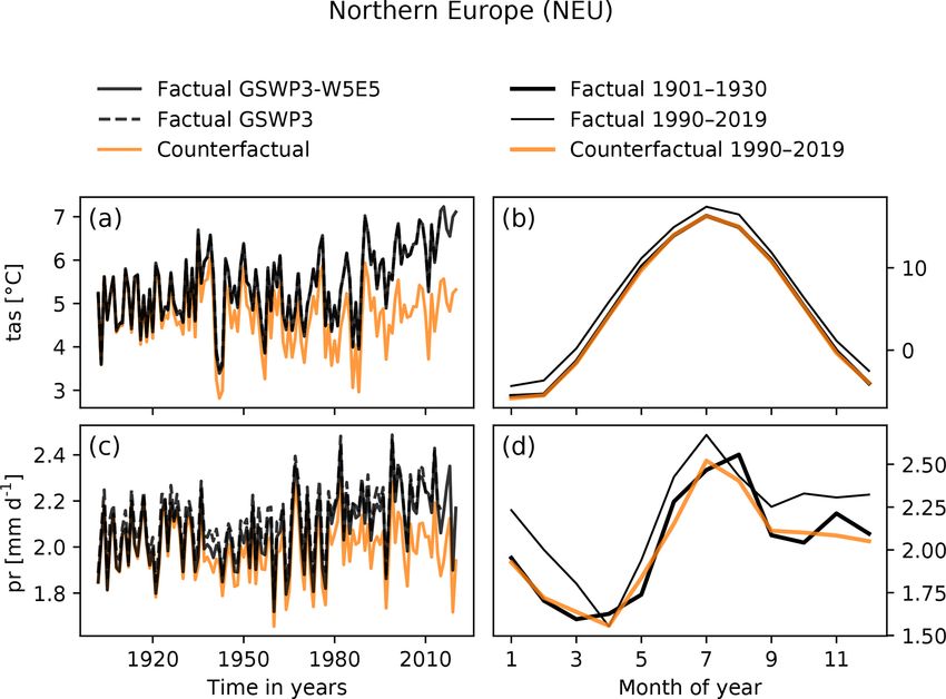
M. Mengel et al.: ATTRICI v1.1                                                                                                      5271

                                                                         pact attribution framework could then be used to approxi-
                                                                         mate the contribution of climate change to observed trends
                                                                         in reported damages. Using process-based climate impact
                                                                         models, this contribution can be explicitly separated from
                                                                         changes in damages driven by changes in exposure or vul-
                                                                         nerability. In this regard it goes beyond available approaches
                                                                         of damage attribution that simply estimate the contribution
                                                                         of anthropogenic climate forcing to observed damages by
                                                                         multiplying the fraction of attributable risk associated with
                                                                         weather extremes by the observed damage (Frame et al.,
                                                                         2020). In the same way, it could improve the attribution of
                                                                         health impacts (Mitchell et al., 2016).
Figure 2. Attribution of impact event magnitude and trends in im-           In this paper we introduce a detrending method tai-
pact indicators to trend in climate. First, in an evaluation step it     lored to support impact attribution and illustrate its ap-
has to be demonstrated that historical impact observations (black        plication to one of the observational climate datasets pro-
line) can be explained by the process understanding as represented       vided within ISIMIP3a (https://protocol.isimip.org/protocol/
in the applied impact model and available knowledge about his-           ISIMIP3a, last access: 4 August 2021; see Sect. 2 below).
torical climate and socio-economic forcings. To this end, the fac-       The quality of the associated impact attribution studies will
tual simulations forced by historical climate and socio-economic         critically depend on the quality of that observational dataset.
forcings (solid blue line) are compared to the impact observations
                                                                         Deficits in the observational data may lead to artifacts in the
(solid black line). Secondly, in the attribution step the impact model
                                                                         derived historical trends. For the dataset used here, we iden-
is driven by counterfactual climate while all other drivers are kept
equal to the factual simulation (counterfactual simulation; solid or-    tify some of those artifacts. Since it is expected that other ar-
ange line). A comparison between factual and counterfactual simu-        tifacts will be found for other observational datasets, impact
lations allows for the attribution of long-term changes (e.g., trends)   attribution studies should ideally be based on a range of dif-
in the impact indicator to trends in climate (contribution to trend,     ferent observational datasets to facilitate a quantification of
CT). In addition, the contribution of climate change to the magni-       the contribution of observational climate data uncertainty to
tude of individual events (impact event attribution) can be deter-       the uncertainty of the attribution results. This is also planned
mined as the difference between the simulated factual event magni-       within ISIMIP3a. For the dataset considered here and poten-
tude and the counterfactual impact event magnitude (CE).                 tial additional ones we propose a collection of control plots
                                                                         that should be used to scan the observational climate data
                                                                         for artifacts in preparation of each individual impact attribu-
but otherwise the same input as in the factual simulation.               tion study. While we provide the control plots for a set of
Such a comparison allows for a quantification of the con-                large-scale world regions and all climate variables covered
tribution of climate change to both the observed trend in the            by our observational climate dataset, they should be adjusted
impact indicator (CT in Fig. 2) and the observed magnitude               to the regions and variables of interest in an impact attribu-
of an individual impact event (CE in Fig. 2). This assumes               tion study as part of the analysis of the factual impact simu-
that the climate impact model calibrated to perform well in              lation (Fig. 2). Low-quality factual climate forcing data are
the factual simulation performs robustly also with counter-              expected to result in a low-quality reproduction of observed
factual climate input data.                                              variations in the impact indicators of interest. If that is the
    Process-based impact models such as those taking part in             case, the simulation setup outlined here does not allow for
the ISIMIP project (http://www.isimip.org, last access: 4 Au-            an attribution of the observed changes in impacts to climate
gust 2021) are ideal tools to address impact attribution as              change.
they generally describe the response of natural, human or
managed systems not only to climate but also direct (human)
drivers. For example, crop models can simulate the response              2   Data
of crop yields to changes in land use, irrigation patterns, fer-
tilizer input and crop varieties (Lobell et al., 2011; Challi-           For ISIMIP3a, we construct counterfactual climate data for
nor et al., 2014; Minoli et al., 2019). Similarly, hydrologi-            the global observational dataset GSWP3-W5E5. This dataset
cal models can be used to simulate how dam construction                  has daily temporal and 0.5◦ spatial resolution and consists of
and water withdrawal affect river discharge (Veldkamp et al.,            two parts: W5E5 v2.0 for the period 1979–2019 and GSWP3
2017, 2018). In addition, those models allow for a process-              v1.09 homogenized with W5E5 for the period 1901–1978.
based representation of the extent of, e.g., river floods and            In the following, we describe these two parts as well as why
droughts that can be combined with maps of asset distribu-               and how they were combined for ISIMIP3a.
tion and empirical damage functions to estimate the direct                  The GSWP3 v1.09 dataset is from the third phase of
economic damages induced by weather extremes. The im-                    the Global Soil Wetness Project (GSWP3), an ongoing land

https://doi.org/10.5194/gmd-14-5269-2021                                                   Geosci. Model Dev., 14, 5269–5284, 2021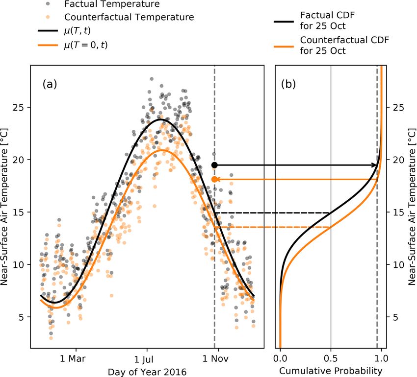
5272                                                                                          M. Mengel et al.: ATTRICI v1.1

model intercomparison project, which shares its experiment        shortwave radiation. Since those estimates are only avail-
protocol with “land-hist” of the Land Surface, Snow and Soil      able for 1983–2007, bias-adjusted daily values were com-
moisture Model Intercomparison Project (LS3MIP; van den           puted as the sum of a rescaled monthly mean value and a
Hurk et al., 2016) and covers the years 1901–2014 (Kim,           rescaled daily anomaly from the monthly mean, with the
2017). It is a dynamically downscaled and bias-adjusted ver-      rescaling done such that, for the 1983–2007 time period, both
sion of the 20th Century Reanalysis (20CR; Compo et al.,          the monthly mean climatology and the anomaly standard-
2011) and has been used as a meteorological forcing dataset       deviation climatology matched the respective SRB estimates.
in several climate impact assessments such as those carried       Wind speed was bias-adjusted at the monthly timescale over
out in ISIMIP2a (e.g., Müller Schmied et al., 2016; Chang et      land using mean monthly climatologies from the Climatic
al., 2017; Schewe et al., 2019; Padrón et al., 2020) as well as   Research Unit (CRU) CL2.0 dataset (New et al., 2002). The
in broader modeling studies (e.g., Krinner et al., 2018; Tang-    bias adjustment was done by monthly rescaling such that
damrongsub et al., 2018; Tokuda et al., 2019). GSWP3 is           the 1961–1990 mean monthly climatology matched that of
also provided for the impact model evaluation task within         CRU CL2.0. Temperature, pressure and humidity were bias-
ISIMIP3a.                                                         adjusted at the 3-hourly timescale using the WATCH forcing
   20CR assimilates subdaily surface pressure and sea-level       data methodology (Weedon et al., 2014) and monthly mean
pressure observations and uses monthly sea-surface tem-           temperatures plus monthly mean diurnal temperature ranges
perature (SST) and sea-ice distributions from the Hadley          from the CRU TS3.23 dataset (Harris et al., 2014), which
Centre Sea Ice and Sea Surface Temperature dataset                covers the full 1901–2014 time period.
(HadISST; Rayner et al., 2003) as lower boundary con-                 As a consequence of its derivation, the quality of the
ditions. To produce GSWP3, the first of the 56 mem-               GSWP3 data varies over time. It varies in line with vari-
bers of the 20CR ensemble was dynamically downscaled              ations in the availability of the pressure, SST and sea-ice
to T238 (about 0.5◦ ) spatial resolution using the incre-         observations used to produce 20CR (Compo et al., 2011;
mental correction of a single member (ICS) method of              Rayner et al., 2003) as well as with variations in the avail-
Yoshimura and Kanamitsu (2013) and the Scripps Institu-           ability of the precipitation and temperature observations used
tion of Oceanography (SIO)/Experimental Climate Predic-           to bias-adjust GSWP3 (Schneider et al., 2014; Weedon et
tion Center (ECPC) Global Spectral Model (GSM) with               al., 2014). Examples of temporal inhomogeneities in GSWP3
spectral nudging (Yoshimura and Kanamitsu, 2008) and ver-         that are relevant for this study include artificial drying trends
tically weighted damping coefficients (Hong and Chang,            over northwest China and the Tibetan Plateau over the first
2012). The ICS method additively adjusts the prognostic           half of the 20th century (Fig. 10) that are inherited from
fields of a single ensemble member such that at the monthly       GPCC (Chen and Frauenfeld, 2014) and spurious trends in
timescale each adjusted field is identical to the correspond-     shortwave radiation and wind speed over Alaska, Northern
ing ensemble mean field while all higher-frequency parts of       Canada and Greenland over the first half of the 20th century
the fields are retained. Hence, the adjusted fields represent     (Figs. 9 and S12 in the Supplement), which are related to ar-
the 20CR best estimates at the monthly timescale while they       tificial extratropical cyclone trends in 20CR over that time
do not suffer from the increase in synoptic variability over      period (Wang et al., 2013). Generally, the quality of 20CR,
time found in the 20CR ensemble mean (Compo et al., 2011)         and hence GSWP3, becomes relatively stable around mid-
that is due to a decrease in the ensemble spread over time,       century over the Northern Hemisphere, earlier over Europe
which in turn reflects the increase in available observational    and later over the Southern Hemisphere, in line with varia-
constraints (Yoshimura and Kanamitsu, 2013).                      tions in the availability of pressure observations for data as-
   The downscaled 3-hourly data were then bilinearly inter-       similation in the reanalysis (Compo et al., 2011).
polated from T238 to a regular 0.5◦ latitude–longitude grid.          The W5E5 v2.0 dataset (Lange et al., 2021) was com-
In addition, selected variables (precipitation, surface down-     piled to support the bias adjustment of climate input data car-
welling shortwave and longwave radiation, near-surface            ried out within ISIMIP3b and covers the years 1979–2019. It
wind speed, near-surface air temperature, surface air pres-       combines the WFDE5 v2.0 dataset (WATCH Forcing Data
sure, and near-surface specific humidity) were bias-adjusted      methodology applied to ERA5 reanalysis data; Cucchi et al.,
with different methods and observational reference datasets.      2020) over land with data from the latest version of the Eu-
Precipitation was bias-adjusted at the monthly timescale us-      ropean Reanalysis (ERA5; Hersbach et al., 2020) over the
ing an undercatch-corrected version of the Global Precipita-      ocean. WFDE5 is a meteorological forcing dataset based on
tion Climatology Centre (GPCC) Full Data Monthly Product          ERA5. For the variables included, it is a spatially aggregated
Version 7 (Schneider et al., 2014). The bias adjustment was       (to 0.5◦ ) and bias-adjusted version of ERA5. Compared to
done by rescaling all monthly mean values to the GPCC esti-       20CR used for GSWP3, many more observations were used
mates. Radiation was bias-adjusted at the daily timescale us-     for data assimilation in ERA5, including precipitation ob-
ing Surface Radiation Budget (SRB; Stackhouse et al., 2011)       servations (Hersbach et al., 2020). That is why we consider
primary-algorithm estimates of daily mean values from SRB         ERA5 to better represent reality than 20CR for 1979 on-
release 3.1 for longwave radiation and SRB release 3.0 for        wards. Similarly, WFDE5 is considered to better represent

Geosci. Model Dev., 14, 5269–5284, 2021                                            https://doi.org/10.5194/gmd-14-5269-2021
M. Mengel et al.: ATTRICI v1.1 5273
reality than GSWP3, in particular with respect to day-to-day
variability for variables that were bias-adjusted using only
monthly mean values in both datasets, such as temperature
and precipitation.
Since W5E5 is considered the more realistic dataset but
only covers 1979–2019, it was extended backward in time
to generate GSWP3-W5E5 for ISIMIP3a. In this extended
dataset, GSWP3 data for 1901–1978 were homogenized with
W5E5 data using the ISIMIP2BASD v2.5 quantile mapping
method (Lange, 2019, 2021). The resulting GSWP3-W5E5
data are identical to the original W5E5 data from 1979 on-
wards but different from the original GSWP3 data before
1979. The goal of the homogenization was to smooth the
transition from one dataset to the other in 1978/1979. To that
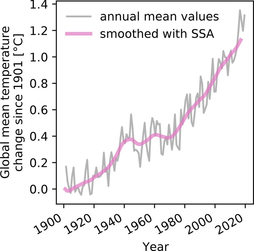
end, for every climate variable and grid cell individually, the Figure 3. Time series of GMT change since 1901 derived from
original GSWP3 time series for 1901–2004 were quantile- GSWP3-W5E5 near-surface air temperature data. Shown are an-
mapped to time series which have the same trends but whose nual mean GMT change (gray) and GMT change smoothed by SSA
with a smoothing window of 10 years (pink). The smoothed GMT
distributions match those of the corresponding W5E5 data
change is used as the predictor of regional climate change in our
over the 1979–2004 reference period. The resulting, homog-
detrending model (denoted by T in the text).
enized GSWP3 data for 1901–1978 were then used to ex-
tend W5E5 backward in time. The preservation of trends im-
plies that differences between trends in GSWP3 and W5E5
data were not homogenized. Consequently, some inhomo- We go beyond this very basic approach by (i) using global
geneities at the 1978/1979 transition remain. This problem mean temperature change instead of time as a potentially
particularly affects surface downwelling shortwave radiation powerful predictor of regional changes in climate, (ii) al-
over northern Europe and the Mediterranean Basin (Fig. 8) lowing for non-normal distributions of the unexplained ran-
as discussed further in the results section. dom year-to-year fluctuations of data per day of the year, and
(iii) ensuring a smooth variation of estimated model parame-
ters from one day of the year to the other.
3 Methodology The use of GMT change, T , as the predictor of regional
climate change is motivated by the classical pattern scaling
Assuming that “climate change refers to any long-term trend
approach (Santer et al., 1990; Mitchell, 2003), with newer
in climate, irrespective of its cause” (IPCC, 2014, chap. 18),
approaches including additional predictors such as a distinc-
we here present a method to generate time series of station-
tion between land and sea to improve accuracy (Herger et
ary climate data from observational daily data by removing
al., 2015). Here, T is GMT change since 1901 smoothed by
the long-term trend while preserving the internal day-to-day
singular spectrum analysis (SSA, Ghil et al., 2002) with a
variability. In the following, we first describe the general
smoothing window of 10 years (Fig. 3). The smoothing of the
characteristics of our approach followed by a more detailed
predictor is applied because we only want to remove long-
formal description of the method. Then we introduce the set
term trends from the regional climate time series. Natural
of global and regional evaluation plots we recommend to re-
climate variability on shorter timescales due to phenomena
gionally adjust and consider within each attribution study us-
such as the El Niño–Southern Oscillation is retained.
ing the counterfactual data generated here or when applying
Using T as the predictor means that we remove long-term
the detrending approach to other observational climate data.
trends in regional climate to the extent that those are cor-
3.1 Detrending method related with GMT change, but irrespective of the cause of
global warming. The success of the detrending is evaluated
A very basic detrending approach would fit a linear temporal by a number of control measures described in Sect. 3.3.
trend for all data of each day of the year assuming normally For each day of the year t the detrending is done with
distributed residuals and remove the estimated trends from quantile mapping (Wood et al., 2004; Cannon et al., 2015;
the data for each day of the year separately. In this approach Lange, 2019) from the factual distribution A (T , t) to the
the trend estimates would not only vary according to system- counterfactual distribution A (T = 0, t). The dependence of
atic variations in trends from one day of the year to the other A on T is modeled via the expected value µ of the distribu-
but also randomly fluctuate from one day of the year to the tion, using a generalized linear model (GLM) or beta regres-
next one in terms of the uncertainties associated with the in- sion (Ferrari and Cribari-Neto, 2004) with a link function g
dividual estimates. defined by g (µ (T , t)) = c0 (t) + c1 (t) T . The link function
g is used to account for climate variables that can only be
https://doi.org/10.5194/gmd-14-5269-2021 Geosci. Model Dev., 14, 5269–5284, 2021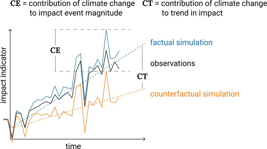
5274                                                                                                     M. Mengel et al.: ATTRICI v1.1

                                                                                                                  (intercept)
positive (in that case, g (x) = ln (x)) or can only take val-           standard deviation of 1.0 for a0                    ; a standard devia-
ues between 0 and 1 (in that case, g (x) = ln (x/ (1 − x))).                                         (intercept)
                                                                        tion of 1/ (2k − 1) for ak               , k = 1, . . ., 4; and a standard
In all other cases g (x) = x. See Table 1 for an overview of                                      (slope)
                                                                        deviation of 0.1 for ak           , k = 0, . . ., 4. Our choice of pri-
which distributions and link functions are used for the dif-                      (intercept)
ferent climate variables, and see Sect. 3.2 for further details.        ors for ak            is based on the assumption that the first
For variables modeled by a Gaussian distribution, the vari-             mode with a period of 1 year explains the largest part of
ance σ 2 of A is assumed to stay constant for each day of               the annual cycle and higher-order modes have decreasing in-
the year; i.e., σ 2 does not vary with T but only depends on            fluence. However this is only a prior assumption; i.e., if the
t. For non-Gaussian distributions, the variance is assumed to           data show different patterns, they can still be captured by our
                                                                                       (constant)                                        (intercept)
change with the expected value. In that case we assume the              model. For ak             we use the same priors as for ak                   .
shape of the distribution to stay constant for each day of the          We use the same priors for the parameters bk . We technically
year.                                                                   implemented the model fitting by use of the pymc3 python
   We use harmonics for the representation of the annual cy-            package (Salvatier et al., 2016). Before the regression, all
cle, i.e., the dependence of the coefficients c0 (t) and c1 (t)         time series are normalized to simplify the Bayesian model
on the day of the year t. Specifically, we use                          parameter estimation. To restore the original units, the nor-
                          Xn                                            malization is reversed after detrending.
g (µ (T , t)) = a0 (T ) +       a (T ) cos (kωt)
                             k=1 k
                                                                           The overall intention of our approach is to find appropri-
                                                                        ate parameter values such that A (T , t) captures long-term
   + bk (T ) sin (kωt)                                            (1)
                                                                        trends in the variables that can be removed by setting T to
                                                      2π
to model the dependence of µ on T and t. Here, ω = 365.25               zero. This is important because the counterfactual distribu-
and n = 4 Fourier modes are used to model the annual cy-                tions are then defined by A (T = 0, t). As an example, the
cle. The GMT-change dependence of the Fourier coefficients              factual µ (T , t) and the counterfactual µ (T = 0, t) as well as
ak , bk is modeled linearly,                                            the associated daily values of one particular tas time series
                                                                        are shown in Fig. 4. The difference between the expected
            (slope)         (intercept)                                 values of distribution A (T , ·) (black line) and A (T = 0, ·)
ak (T ) = ak          T + ak              ; k = 0, 1, . . ., n,   (2)
                                                                        (orange line) is due to a vertical shift that is composed of a
and similarly for b1 , b2 , . . ., bn .                                 linear increase with T captured by a0 and a change in the am-
   The distribution parameters that only depend on t are mod-           plitude and phase of the annual cycle captured by the Fourier
eled using                                                              coefficients ak and bk , k > 0. The counterfactual daily data
              (constant)
                           Xn            (constant)
                                                                        are generated by quantile mapping; i.e., an observed value
ln (ν (t)) = a0          +        k=1 k
                                       a            cos (kωt)           x that corresponds to a certain quantile of the factual distri-
       (constant)                                                       bution A (T , t) is mapped to the counterfactual value x 0 that
   + bk             sin (kωt) ,                                   (3)
                                                                        corresponds to the same quantile of the counterfactual distri-
where ω and n have the same values as in Eq. (1), and ν                 bution A (T = 0, t). We illustrate this for an observed value
represents σ for the Gaussian distribution, k for the gamma             x that corresponds to the 95th percentile of the factual dis-
distribution, α for the Weibull distribution and φ for the beta         tribution in Fig. 4: we first obtain the cumulative probability
distribution (see Table 1 and Sect. 3.2).                               of the factual (i.e., observed) temperature (large black dot
    By limiting the number of Fourier modes to four we re-              in panel a) from the factual cumulative distribution function
duce the number of coefficients to be estimated and ensure a            (CDF; black line in panel b). We then obtain the counter-
smooth variation of the long-term trend in µ over the course            factual temperature (large orange dot in panel a) from the
of the year but still capture seasonal to sub-seasonal patterns         counterfactual CDF (orange line in panel b).
such as monsoon season onsets. Setting n = 4 in Eq. (1) leads
to a total of 18 slope and intercept parameters to describe the         3.2     Model choices for each climate variable
expected value µ in terms of T and t. Setting n = 4 in Eq. (3)
                                                                        3.2.1    Near-surface air temperature, surface air
means that nine parameters are used to describe the depen-
                                                                                 pressure and surface downwelling longwave
dence of σ , k, α and φ on t.
                                                                                 radiation
    We use a Bayesian approach to estimate all of these param-
eters. This requires the specification of prior distributions of        We use the Gaussian distribution to model these variables as
the model parameters. Similar to regularization techniques in           their values are far from their physical lower bound of zero.
frequentist approaches, the prior allows us to focus the model
fitting on plausible parameter values. This is particularly im-
portant for numeric stability when the logit and logarithm
link functions are applied. We use a zero-centered Gaussian
prior for all parameters and all climate variables because we
normalize the data before parameter estimation. We use a

Geosci. Model Dev., 14, 5269–5284, 2021                                                     https://doi.org/10.5194/gmd-14-5269-2021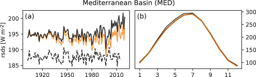
M. Mengel et al.: ATTRICI v1.1                                                                                                           5275

Table 1. Climate variables covered by ISIMIP3a counterfactual climate datasets. Listed are each variable’s short name and unit as well as
the statistical distribution and link function used for detrending it. Also specified is the dependence of the distribution parameters on GMT
change, T , and day of the year, t, as used in our GLM. The variables tasrange and tasskew are auxiliary variables used to detrend tasmin and
tasmax.

        Variable                             Short name     Unit           Statistical distribution            Link function
        Daily mean near-surface              tas            K              Gaussian with mean value            g (µ) = µ
        air temperature                                                    µ (T , t) and standard deviation
                                                                           σ (t)
        Daily near-surface temperature       tasrange       K              Gamma with mean value               g (µ) = ln (µ)
        range                                                              µ (T , t) and shape k (t)
        Daily near-surface temperature       tasskew        1              Gaussian with mean value            g (µ) = µ
        skewness                                                           µ (T , t) and standard deviation
                                                                           σ (t)
        Precipitation                        pr             kg m−2 s−1     For wet or dry day: Bernoulli       g (p) = ln (p/ (1 − p))
                                                                           with      dry-day     probability
                                                                           p (T , t)
                                                                           For intensity of precipitation on   g (µ) = ln (µ)
                                                                           wet days: gamma with mean
                                                                           value µ (T , t) and shape k (t)
        Surface downwelling shortwave        rsds           W m−2          Gaussian with mean value            g (µ) = µ
        radiation                                                          µ (T , t) and standard deviation
                                                                           σ (t)
        Surface downwelling longwave         rlds           W m−2          Gaussian with mean value            g (µ) = µ
        radiation                                                          µ (T , t) and standard deviation
                                                                           σ (t)
        Surface air pressure                 ps             Pa             Gaussian with mean value            g (µ) = µ
                                                                           µ (T , t) and standard deviation
                                                                           σ (t)
        Near-surface wind speed              sfcwind        m s−1          Weibull with shape α (t) and        g (β) = ln (β)
                                                                           scale β (T , t)
        Near-surface relative humidity       hurs           %              Beta with mean value                g (µ) = ln (µ/ (1 − µ))
                                                                           µ (T , t) and dispersion φ (t)
        Near-surface specific humidity       huss           kg kg−1        Derived from hurs, ps and tas
        Daily minimum near-surface air       tasmin         K              Derived from tas, tasrange and tasskew
        temperature
        Daily maximum near-surface air       tasmax         K              Derived from tas, tasrange and tasskew
        temperature

3.2.2    Daily minimum and maximum near-surface air                      use the gamma distribution to model tasrange since it has a
         temperature                                                     lower bound at zero. The expected value is modeled accord-
                                                                         ing to Eq. (1). The skewness of the diurnal near-surface tem-
                                                                         perature cycle, tasskew, is modeled by a Gaussian distribu-
They provide a measure of the diurnal temperature cycle in
                                                                         tion. While theoretically bounded, tasskew is never close to
the daily resolved dataset. We do not estimate counterfac-
                                                                         its bounds of zero and one. This justifies the Gaussian model
tual time series for tasmin and tasmax directly to avoid large
                                                                         choice.
relative errors in the daily temperature range as pointed out
by Piani et al. (2010). Instead we construct counterfactuals
for the auxiliary variables tasrange = tasmax − tasmin and
tasskew = (tas − tasmin)/tasrange that then determine the
tasmin and tasmax counterfactuals (Piani et al., 2010). We

https://doi.org/10.5194/gmd-14-5269-2021                                                     Geosci. Model Dev., 14, 5269–5284, 2021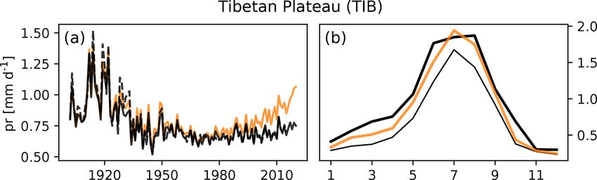
5276                                                                                               M. Mengel et al.: ATTRICI v1.1

                                                                       climate variables. These inconsistencies are small by design
                                                                       since the new wet days are the least wet of all counterfactual
                                                                       wet days.

                                                                       3.2.4    Surface downwelling shortwave radiation

                                                                       Physically bound to positive numbers, the limit is only
                                                                       reached in the special case of the polar night. We thus use
                                                                       a Gaussian distribution to model rsds. If quantile mapping
                                                                       leads to negative values, we use the original value instead.

                                                                       3.2.5    Near-surface wind speed

                                                                       We use a Weibull distribution to model surface wind speed.
                                                                       The distribution has a shape parameter α and a scale pa-
                                                                       rameter β, which both need to be positive. The expected
                                                                       value of the Weibull distribution is given by β0 (1 + 1/α)
                                                                       with the gamma function 0. We model the scale parameter
                                                                       β by Eq. (1) using the natural logarithm as the link function.
                                                                       We handle the shape parameter similar to the standard devia-
Figure 4. Illustration of detrending with quantile mapping sensitive   tion of the Gaussian distribution, being independent of GMT
to the annual cycle. Panel (a) shows the factual (black points) and    change but varying with t.
counterfactual (orange points) daily mean near-surface air tempera-
ture data for the year 2016 of GSWP3-W5E5 for a single grid cell       3.2.6    Near-surface relative humidity
in the Mediterranean region at 43.25◦ N, 5.25◦ E. In panel (a), the
black and orange lines show the temporal evolution of the expected     Near-surface relative humidity hurs is positive and less than
value µ of the factual and the counterfactual distribution. In panel   or equal to one. We assume hurs to follow a beta distribu-
(b), the black and orange lines show the factual and counterfactual    tion. Its expected value is allowed to vary with T and t.
cumulative distribution function (CDF) for a single day (25 Octo-      The associated coefficients are estimated using a beta regres-
ber 2016). The large points on the dashed vertical line in panel (a)   sion model (Ferrari and Cribari-Neto, 2004) and Eq. (1) for
highlight the factual (large black point) and counterfactual (large
                                                                       the expected value, while the dispersion parameter, φ, is as-
orange point) value on 25 October. They correspond to the 95th
                                                                       sumed to only vary with t.
percentile in their respective distributions.
                                                                       3.2.7    Near-surface specific humidity
3.2.3   Precipitation                                                  The counterfactual for huss is derived from counterfactual
                                                                       tas, ps and hurs using the equations of Buck (1981) as de-
We use a mixed Bernoulli–gamma distribution (Gudmunds-                 scribed in Weedon et al. (2010).
son et al., 2012) for precipitation; i.e., the distribution of wet
versus dry days is described by a Bernoulli distribution with          3.3     Evaluation method
p describing the probability of dry days, while the intensity
of precipitation on wet days is assumed to follow a gamma              To evaluate the detrending method and the counterfactual
distribution. A day is considered dry if the amount of pre-            GSWP3-W5E5 data, we use the difference between multi-
cipitation is below 0.1 mm d−1 . Wet days are all days where           year averages of each climate variable over the beginning of
the threshold is exceeded. We describe the gamma distribu-             the time period (1901–1930) and multi-year averages over
tion by its expected value and a shape parameter k. We as-             the end of the time period (1990–2019) as a measure of the
sume that the expected value, p, of the Bernoulli distribution         trend. We compare this trend measure between the observed
and the expected value of the gamma distribution vary with             data and the counterfactual data, for which it should be close
T and t, while the shape parameter k of the gamma distri-              to zero (Figs. 5 and 6). In addition, we propose plotting the
bution is assumed to only vary with t. If the probability of           entire time series for regionally averaged annual (or seasonal)
dry days, pfactual , of the factual distribution A (T , t) is larger   mean values for both the original and the counterfactual cli-
than the probability of dry days, pcounterfactual , of the coun-       mate data. Here, we do so for annual regional averages over
terfactual distribution A (T = 0, t), dry days are turned into         21 world regions (Giorgi and Francisco, 2000), see left pan-
wet days at random with probability pfactual − pcounterfactual         els of Figs. 7–10 and Supplement figures, but propose ad-
by assigning them a small precipitation amount above the               justing the regions and season for each attribution study in-
wet-day threshold. This random conversion of dry days into             dividually according to its focus. For our specific observa-
wet days may result in physical inconsistencies with other             tional dataset we add annual regional averages of the original

Geosci. Model Dev., 14, 5269–5284, 2021                                                https://doi.org/10.5194/gmd-14-5269-2021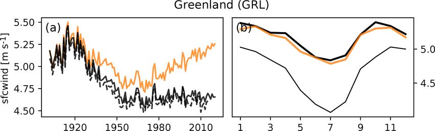
M. Mengel et al.: ATTRICI v1.1                                                                                                5277

GSWP3 data to check if the homogenization of GSWP3 with             age time series (Fig. 7c). There is a seasonality in the long-
W5E5 has introduced artificial trends in the factual GSWP3-         term trend with almost no change in April and August in con-
W5E5 data. To evaluate the performance of the detrending            trast to positive trends in the other months (compare thick to
method for each day of the year we propose to compare the           thin black line in Fig. 7d). Our approach successfully cap-
1990–2019 regional mean climatology of the counterfactual           tures this seasonal variation of the trend. The annual cycle of
data to the 1901–1930 regional mean climatology of the fac-         the counterfactual data in the period 1990–2019 (orange line)
tual data for each region of interest (right panels of Figs. 7–10   matches the annual cycle of the factual data in the beginning
and Supplement figures).                                            of the century 1901–1930 (thick black line).

                                                                    4.3   Shortwave radiation, Mediterranean Basin (MED)
4     Results
                                                                    There is a considerable offset between the GSWP3 and
The counterfactual dataset evaluated in the following is free       W5E5 data in the overlapping 1979–2014 period (see dif-
to download through the ISIMIP data portal (https://data.           ference between dashed and solid black line in Fig. 8). In
isimip.org/search/climate_scenario/counterclim/, last access:       addition, the GSWP3 data do not show a trend over the en-
4 August 2021) along with the underlying original data. Our         tire time period 1901–2014, whereas there is a positive trend
method strongly reduces the observed difference between             in the 1979–2019 W5E5 data. The harmonization has shifted
multi-year averages over the beginning of the century (1901–        the original GSWP3 data but did not introduce a trend by de-
1930) and the end of the observational period (1990–2019)           sign of the quantile mapping method used for it (see Sect. 2).
for most locations and variables (Figs. 5 and 6). The remain-       This results in inhomogeneous decadal trends in the GSWP3-
ing differences are largest for precipitation over the Tibet re-    W5E5 data and a jump at the 1978/1979 transition. This
gion and for wind speed over Greenland. In the following we         change in the characteristics of the shortwave radiation in
exemplarily zoom into these regions to resolve the temporal         GSWP3-W5E5 is an artifact introduced by the different char-
evolution of the regionally averaged factual and counterfac-        acteristics of the GSPW3 and W5E5 data and not related to
tual data (Figs. 7–10, left panels) and evaluate the detrending     GMT change. Thus, in this region the trend in the factual rsds
for each day of the year (Figs. 7–10, right panels). We start       time series is not reliable enough to derive a meaningful no-
with temperature and precipitation in northern Europe where         climate-change counterfactual rsds time series. Annual short-
the detrending works well and then focus on regions where           wave radiation over northern Europe is affected in a similar
the factual data show artifacts that may make them inade-           way (Fig. S21).
quate for impact attribution within the proposed setup.
                                                                    4.4   Wind speed, Greenland (GRL)
4.1    Temperature, northern Europe (NEU)
                                                                    The factual datasets show spurious trends in wind speed over
There is essentially no difference between the GSWP3 data           Alaska, northern Canada and Greenland over the first half of
and the GSWP3-W5E5 data in the period 1979–2014 where               the 20th century (regions GRE and ALA, Figs. 9 and S16),
the original GSWP3 and W5E5 data overlap. Our approach              which are related to artificial extratropical cyclone trends
successfully removes the long-term trend from the observed          in the 20CR reanalysis over that time period (Wang et al.,
time series of regionally averaged annual temperature data          2013). Shortwave radiation in those regions is affected in a
(Fig. 7a) and for each day of the year (Fig. 7b). By construc-      similar way (Figs. S15 and S17). Our detrending method is
tion, the detrending retains the year-to-year variability; i.e.,    unable to distinguish spurious trends from real trends. It finds
hot days stay hot and cold days stay cold. The counterfactual       a correlation between GMT change and the spurious trends
1990–2019 averages for individual days of the year match            and produces counterfactual data that have a spurious posi-
the seasonal evolution of the factual data at the beginning         tive trend over the second half of the 20th century (Fig. 9a).
of the century (1901–1930) as intended. In northern Europe,         Such counterfactual time series are clearly not reliable.
temperatures for each day of the year have changed relatively
uniformly throughout the year (Fig. 7b).                            4.5   Precipitation, Tibetan Plateau (TIB)

4.2    Precipitation, northern Europe (NEU)                         Over the first half of the 20th century the GSWP3-W5E5 pre-
                                                                    cipitation data show a strong drying trend over the TIB region
The GSWP3 data are offset to slightly higher values of pre-         that is assumed to be artificial and inherited from the under-
cipitation compared to the GSWP3-W5E5 data in the period            lying GPCC dataset (Sect. 2). Since the trend is not related
1979–2014 where the original GSWP3 and W5E5 data over-              to global warming, it is not well captured by our detrending
lap. The homogenization method of the GSWP3-W5E5 data               model. Consequently, the average counterfactual precipita-
transfers this offset to the period 1901–1979, leading to a         tion at the end of the observational period does not match the
more consistent dataset. Our approach successfully removes          average factual data at the beginning of the period (Figs. 5h
the long-term trend from the observed annual regional aver-         and 10b). The detrending leads to a positive trend over the

https://doi.org/10.5194/gmd-14-5269-2021                                              Geosci. Model Dev., 14, 5269–5284, 2021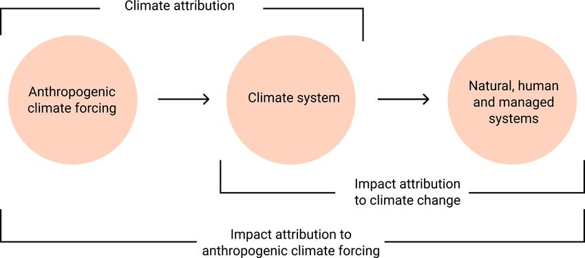
5278                                                                                                M. Mengel et al.: ATTRICI v1.1

Figure 5. Differences between multi-year averages over the late (1990–2019) and early (1901–1930) time period for the factual (left) and
counterfactual (right) GSWP3-W5E5 dataset. Results are shown for tas, tasmin, tasmax, pr and rsds (from top to bottom). Rectangles show
the 21 world regions from Giorgi and Francisco (2000). Note that the color scale is capped for precipitation; i.e., values below −2 mm d−1
and above 2 mm d−1 are displayed in dark blue and dark red, respectively.

second half of the century, while the factual data do not show         evolving drivers. Impact attribution as defined in the intro-
such a trend. Since the observational data for the first half of       duction aims to quantify the role of climate change versus
the century are considered unreliable, they are also not fit to        the other drivers of change. Impact attribution needs a com-
derive a meaningful no-climate-change counterfactual.                  parison of the observed state of the considered system to
   We present further plots covering all variables and Giorgi          its hypothetical, counterfactual state without climate change.
regions in the Supplement. Given potential artifacts in the            The reason for the change in climate trends and a separation
factual data, the associated plots have to be analyzed when            of anthropogenically forced changes from climate variability
planning a regional attribution study.                                 are not necessarily required. Thus, a simplified methodology
                                                                       that detrends observational data is sufficient without the need
                                                                       for probabilistic climate model simulations. The proposed
5   Discussion                                                         design of the counterfactual climate forcing data and the as-
                                                                       sociated impact simulation framework mean a restriction to
The attribution of changes in the climate system to anthro-            “impact attribution to climate change” instead of “impact at-
pogenic interference with the climate system is a mature re-           tribution to anthropogenic climate forcing”. The latter is nec-
search field (IPCC, 2013; Gillett et al., 2016; NAS, 2016;             essary to, for example, attribute a fraction of an impact to a
Stott et al., 2016). Less work has been done on the attri-             greenhouse gas emitter and support climate litigation (Mar-
bution of changes in natural, human and managed systems                janac et al., 2017; Burger et al., 2020). Thus the counterfac-
affected by climate change in combination with other time-

Geosci. Model Dev., 14, 5269–5284, 2021                                                  https://doi.org/10.5194/gmd-14-5269-2021
M. Mengel et al.: ATTRICI v1.1 5279 Figure 6. Same as Fig. 5 but for rlds, ps, sfcwind, hurs and huss. Note that the color scale is capped for wind at −0.5 and 0.5 m s−1 and for hurs at −12 % and 12 %. Values below and above those bounds are displayed in dark blue and dark red, respectively. tual climate data generated here are not intended to replace the basic IPCC AR5 WGII definition utilizing the strength climate simulations with counterfactual greenhouse gas forc- of impact models to address the important question of to ings such as the histNAT CMIP6 experiments’ (Gillett et al., what degree climate change is already affecting natural, hu- 2016) large climate model ensembles that are required to at- man and managed systems. So far the contribution of cli- tribute changes in climate or impacts to anthropogenic emis- mate change to long-term historical changes in human, nat- sions. ural or managed systems is often addressed by model simu- Climate impact models can be considered as ideal tools lation where direct human interventions are fixed while only to address impact attribution as they are usually designed to climate is allowed to change according to historical obser- represent the response of impact indicators to climate dis- vations (e.g., Sauer et al., 2021). However, this alternative turbances but also account for direct human interventions definition may also lead to different results and does not al- such as agricultural management changes, water abstraction low for the attribution of the magnitude of individual impact or flood protection measures. Within the model, individual events to climate change as described in Fig. 2. drivers can be controlled, and a factual run (observed climate Attribution draws a causal connection and quantifies the change + observed direct human interventions, Fig. 2 blue change due to the cause. An important part of the attribution line) can be compared to a counterfactual run (counterfactual work is thus to ensure that the cause–effect relationship is climate + observed direct human interventions, Fig. 2 orange correctly captured in the model. This requires careful analy- line). sis and model evaluation to show that the change estimated By providing climate forcing data for counterfactual cli- by an impact model is a reliable estimate of the real-world mate impact runs, we facilitate impact attribution following change. Simulated changes need to agree with observed https://doi.org/10.5194/gmd-14-5269-2021 Geosci. Model Dev., 14, 5269–5284, 2021
5280                                                                                                 M. Mengel et al.: ATTRICI v1.1

                                                                         Figure 9. Same as Fig. 7 but for wind speed over Greenland (GRL).

Figure 7. Panels (a) and (c) show annual regional mean time series
                                                                         Figure 10. Same as Fig. 7 but for precipitation over the Tibetan
of factual GSWP3-W5E5 data (solid black line), factual GWSP3
                                                                         Plateau (TIB).
data (dashed black line) and counterfactual GSWP3-W5E5 data (or-
ange line) for near-surface air temperature (a) and precipitation (c)
over northern Europe (NEU). Panels (b) and (d) show multi-year re-
                                                                         tual observational climate data that particularly affect the first
gional mean climatologies for near-surface air temperature (b) and
precipitation (d) of factual and counterfactual GSWP3-W5E5 data          half of the century and prevent impact attribution in the pro-
for NEU. To obtain the counterfactual annual cycle (orange line),        posed framework.
our method aims to map the late factual (thin black line) to the early      Our detrending approach does not guarantee the mainte-
factual (thick black line) annual cycle.                                 nance of physical consistency of different climate variables
                                                                         in the counterfactual datasets in terms of, e.g., energy clo-
                                                                         sure or water budgets. However, the applied quantile map-
                                                                         ping preserves ranks, which means that relatively high values
                                                                         before the mapping are also relatively high after the mapping
                                                                         and similarly for relatively low values. Statistically speak-
                                                                         ing, univariate quantile mapping independently applied to all
                                                                         climate variables preserves the multivariate rank distribution
                                                                         (the copula) over all variables. In that sense the statistical
                                                                         dependence between variables is preserved by our detrend-
Figure 8. Same as Fig. 7 but for shortwave radiation over the            ing method, and the risk of producing physically inconsis-
Mediterranean Basin (MED).                                               tent counterfactual climate data is at least limited. This is
                                                                         critical for the attribution of the extreme event magnitude
                                                                         to observed climate trends (see introduction) because several
changes, and it needs to be ruled out whether this agreement             climate variables can contribute to impact extremes.
is due to confounding factors that drive observed changes but               Here, we deliberately excluded the question of what drives
are not part of the model simulations. The ISIMIP3a histori-             climate change, i.e., the attribution of changes in the climate
cal simulations serve to address these points and demonstrate            system to greenhouse gas emissions, as it often implies a fo-
the explanatory power of impact models as an integral part of            cus on this aspect and less attention is paid to the separa-
the attribution work.                                                    tion of climate change from direct human interventions as
   Our method ultimately builds on the correlation between               drivers of observed changes in natural, human and managed
a regional climate variable and decadal GMT change to re-                systems. The restriction of the research question to “impact
move long-term trends in the regional climate variables with-            attribution to climate change in general” makes the assess-
out implying causality. It is well possible that changes in              ments independent of climate simulations and their poten-
regional climate variables have other reasons than global                tial limitation in reproducing processes relevant for historical
warming such as local effects of land use changes and aerosol            climate change. Instead, the restricted framework is directly
emissions as well as regional characteristics of large-scale             linked to impact model evaluation and the question of how
decadal climate oscillations. However, our study shows that              well we understand the observed changes in human, natu-
GMT change is generally a powerful predictor allowing for                ral and managed systems. This question can most directly be
generating stationary counterfactual climate data. Major de-             addressed by the factual impact simulations proposed here
trending failures seem to be related to artifacts in the fac-            rather than with impact simulations based on simulated his-

Geosci. Model Dev., 14, 5269–5284, 2021                                                   https://doi.org/10.5194/gmd-14-5269-2021
M. Mengel et al.: ATTRICI v1.1 5281
torical climate. In addition, as opposed to large ensembles European Union H2020 SC5-01-2014 (CRESCENDO, grant no.
of climate model simulations, such a dataset is easily inte- 641816). Simon Treu received funding from the European Union
grated into an impact model intercomparison project such as H2020 LC-CLA-03-2018 (RECEIPT, grant no. 820712).
ISIMIP, which includes models of very different computa-
tional costs. In this way the approach allows for an explo- The publication of this article was funded by the
Open Access Fund of the Leibniz Association.
ration of structural uncertainty in climate impact attribution,
based on a multi-impact-model ensemble, combined with a
variety of damage functions where appropriate.
Review statement. This paper was edited by Juan Antonio Añel and
With the methods and data presented here, we aim to reviewed by two anonymous referees.
advance the field of impact attribution and reveal past and
present societal and environmental sensitivities to climate
change. Getting a better understanding of the drivers of ob-
served changes in natural, human and managed systems will
help us to better estimate future risks related to ongoing
References
global warming and develop adequate adaptation measures.
Abatzoglou, J. T. and Williams, A. P.: Impact of anthropogenic cli-
mate change on wildfire across western US forests, P. Natl. Acad.
Code and data availability. The source code underlying
Sci. USA, 113, 11770–11775, 2016.
the analysis presented in the paper (v1.1.0) is archived at
Buck, A. L.: New Equations for Computing Vapor Pressure and En-
https://doi.org/10.5281/zenodo.5032065 (Mengel et al., 2021a).
hancement Factor, J. Appl. Meteorol., 20, 1527–1532, 1981.
The source code to produce the figures as appearing in the paper
Burger, M., Wentz, J., and Horton, R.: The Law and Science of
(v1.1.0) is archived at https://doi.org/10.5281/zenodo.5036701
Climate Change Attribution, Columbia Journal of Environmental
(Mengel and Treu, 2021). All code is open to use under the GPL
Law, 45, 57–240, https://doi.org/10.7916/cjel.v45i1.4730, 2020.
license. The presented counterfactual climate dataset is archived at
Butler, E. E., Mueller, N. D., and Huybers, P.: Peculiarly pleasant
https://doi.org/10.5281/zenodo.5036364 (Mengel et al., 2021b) and
weather for US maize, P. Natl. Acad. Sci. USA, 115, 11935–
based on v1.1.0 of the source code.
11940, 2018.
Cannon, A. J., Sobie, S. R., and Murdock, T. Q.: Bias Correction of
GCM Precipitation by Quantile Mapping: How Well Do Methods
Supplement. The supplement related to this article is available on- Preserve Changes in Quantiles and Extremes?, J. Climate, 28,
line at: https://doi.org/10.5194/gmd-14-5269-2021-supplement. 6938–6959, 2015.
Challinor, A. J., Watson, J., Lobell, D. B., Howden, S. M., Smith, D.
R., and Chhetri, N.: A meta-analysis of crop yield under climate
Author contributions. MM, ST, SL and KF developed the concept. change and adaptation, Nat. Clim. Chang., 4, 287–291, 2014.
ST and MM implemented the methods, wrote the code and pro- Chang, J., Ciais, P., Wang, X., Piao, S., Asrar, G., Betts, R., Cheval-
duced the data. All authors wrote the paper. lier, F., Dury, M., François, L., Frieler, K., Ros, A. G. C., Hen-
rot, A.-J., Hickler, T., Ito, A., Morfopoulos, C., Munhoven, G.,
Nishina, K., Ostberg, S., Pan, S., Peng, S., Rafique, R., Reyer,
Competing interests. The authors declare that they have no conflict C., Rödenbeck, C., Schaphoff, S., Steinkamp, J., Tian, H., Viovy,
of interest. N., Yang, J., Zeng, N., and Zhao, F.: Benchmarking carbon fluxes
of the ISIMIP2a biome models, Environ. Res. Lett., 12, 045002,
https://doi.org/10.1088/1748-9326/aa63fa, 2017.
Disclaimer. Publisher’s note: Copernicus Publications remains Chen, L. and Frauenfeld, O. W.: A comprehensive evaluation of pre-
neutral with regard to jurisdictional claims in published maps and cipitation simulations over China based on CMIP5 multimodel
institutional affiliations. ensemble projections: CMIP5 PRECIPITATION IN CHINA, J.
Geophys. Res., 119, 5767–5786, 2014.
Compo, G. P., Whitaker, J. S., Sardeshmukh, P. D., Matsui, N., Al-
lan, R. J., Yin, X., Gleason, B. E., Vose, R. S., Rutledge, G.,
Acknowledgements. We thank Hyungjun Kim for helping us to ex-
Bessemoulin, P., Brönnimann, S., Brunet, M., Crouthamel, R. I.,
plain the making of the GSWP3 dataset. We thank Anne Gädeke
Grant, A. N., Groisman, P. Y., Jones, P. D., Kruk, M. C., Kruger,
and Christoph Menz for beta testing our counterfactual data. We are
A. C., Marshall, G. J., Maugeri, M., Mok, H. Y., Nordli, Ø., Ross,
grateful to Benjamin Schmidt’s early contributions to the code. We
T. F., Trigo, R. M., Wang, X. L., Woodruff, S. D., and Worley, S.
thank the two anonymous reviewers for their helpful comments on
J.: The Twentieth Century Reanalysis Project, Q. J. Roy. Meteor.
the initial version of this paper.
Soc., 137, 1–28, 2011.
Cucchi, M., Weedon, G. P., Amici, A., Bellouin, N., Lange, S.,
Müller Schmied, H., Hersbach, H., and Buontempo, C.: WFDE5:
Financial support. This research has been supported by the bias-adjusted ERA5 reanalysis data for impact studies, Earth
German Federal Ministry of Education and Research (BMBF, Syst. Sci. Data, 12, 2097–2120, https://doi.org/10.5194/essd-12-
grant no. 01LS1711A). Stefan Lange received funding from the 2097-2020, 2020.
https://doi.org/10.5194/gmd-14-5269-2021 Geosci. Model Dev., 14, 5269–5284, 2021You can also read