Estimation of fire-induced carbon emissions from Equatorial Asia in 2015 using in situ aircraft and ship observations
←
→
Page content transcription
If your browser does not render page correctly, please read the page content below

Atmos. Chem. Phys., 21, 9455–9473, 2021
https://doi.org/10.5194/acp-21-9455-2021
© Author(s) 2021. This work is distributed under
the Creative Commons Attribution 4.0 License.

Estimation of fire-induced carbon emissions from Equatorial Asia in
2015 using in situ aircraft and ship observations
Yosuke Niwa1,2 , Yousuke Sawa2,a , Hideki Nara1 , Toshinobu Machida1 , Hidekazu Matsueda2,b , Taku Umezawa1 ,
Akihiko Ito1 , Shin-Ichiro Nakaoka1 , Hiroshi Tanimoto1 , and Yasunori Tohjima1
1 National Institute for Environmental Studies, Tsukuba, Japan
2 Meteorological  Research Institute, Tsukuba, Japan
a now at: Japan Meteorological Agency, Tokyo, Japan
b now at: Dokkyo University, Soka, Japan

Correspondence: Yosuke Niwa (niwa.yosuke@nies.go.jp)

Received: 4 December 2020 – Discussion started: 23 December 2020
Revised: 5 May 2021 – Accepted: 20 May 2021 – Published: 23 June 2021

Abstract. Inverse analysis was used to estimate fire carbon       1   Introduction
emissions in Equatorial Asia induced by the big El Niño
event in 2015. This inverse analysis is unique because it ex-
tensively used high-precision atmospheric mole fraction data      Equatorial Asia, which includes Indonesia, Malaysia, Papua
of carbon dioxide (CO2 ) from the commercial aircraft obser-      New Guinea and the surrounding areas (Fig. 1) has experi-
vation project CONTRAIL. Through comparisons with in-             enced extensive biomass burning, especially during drought
dependent shipboard observations, especially carbon monox-        conditions induced by El Niño and the Indian Ocean dipole
ide (CO) data, the validity of the estimated fire-induced car-    (Field et al., 2009). This biomass burning has emitted a sig-
bon emissions was demonstrated. The best estimate, which          nificant amount of carbon, mainly in the form of carbon diox-
used both aircraft and shipboard CO2 observations, indicated      ide (CO2 ), into the atmosphere (Page et al., 2002; Patra et
273 Tg C for fire emissions from September–October 2015.          al., 2005; van der Werf et al., 2008). Much of these fire-
This 2-month period accounts for 75 % of the annual total fire    induced carbon emissions in Equatorial Asia came from peat-
emissions and 45 % of the annual total net carbon flux within     land, which has a remarkably high carbon density. Since the
the region, indicating that fire emissions are a dominant driv-   peatland in Equatorial Asia accounts for a significant portion
ing force of interannual variations of carbon fluxes in Equa-     of the global peatland (Page et al., 2011), the region has a
torial Asia. Several sensitivity experiments demonstrated that    distinct role in the global carbon cycle despite its small ter-
aircraft observations could measure fire signals, though they     restrial coverage.
showed a certain degree of sensitivity to prior fire-emission        In 2015, the extreme El Niño, accompanied by a pos-
data. The inversions coherently estimated smaller fire emis-      itive anomaly of the Indian Ocean dipole, induced se-
sions than the prior data, partially because of the small con-    vere drought and devastating biomass burning in Equato-
tribution of peatland fires indicated by enhancement ratios       rial Asia. This was one of biggest El Niño events in the
of CO and CO2 observed by the ship. In future warmer cli-         last 30 years, rivalling the well-known major El Niño in
mate conditions, Equatorial Asia may experience more se-          1997/1998 (L’Heureux et al., 2017; Santoso et al., 2017).
vere droughts, which risks releasing a large amount of carbon     Page et al. (2002) estimated that the biomass burning in 1997
into the atmosphere. Therefore, the continuation of aircraft      emitted a massive amount of carbon into the atmosphere,
and shipboard observations is fruitful for reliable monitoring    ranging between 810 and 2570 Tg C.
of carbon fluxes in Equatorial Asia.                                 Compared to 1997, more observations were available in
                                                                  2015, and several studies used those observations to esti-
                                                                  mate the fire-induced carbon emissions. Field et al. (2016)
                                                                  reported that the annual total carbon emissions induced by

Published by Copernicus Publications on behalf of the European Geosciences Union.
9456                              Y. Niwa et al.: Estimation of fire-induced carbon emissions from Equatorial Asia in 2015

                                                                    2008; Crisp, 2015) and obtained a CO2 emissions estimate of
                                                                    748 Mt CO2 (equivalent to 204 Tg C) from July to November
                                                                    2015, which covers the beginning and end of the fire season.
                                                                    Their estimate was 35 % and 30 % smaller than the MODIS-
                                                                    based emission estimates of GFED4s and GFAS v1.2, re-
                                                                    spectively. This lower estimate is more consistent with the
                                                                    estimate of Huijnen et al. (2016) than that of Yin et al. (2015).
                                                                       Thus, the estimates of the fire-induced carbon emissions
                                                                    in Equatorial Asia for 2015 are still uncertain, though they
                                                                    are consistently much smaller than those of 1997. As dis-
                                                                    cussed by Field et al. (2009, 2016) and Yin et al. (2016),
                                                                    a nonlinear sensitivity of the fire emissions to the climate
                                                                    conditions contributed to the notable discrepancy of the fire-
                                                                    emission amount between 1997 and 2015. However, the un-
                                                                    derlying mechanisms are unclear, and further investigation
                                                                    and a more accurate emissions estimate are required. Impor-
                                                                    tantly, the previous studies mainly relied on satellite data of
Figure 1. Locations of the observations obtained by CONTRAIL        atmospheric CO2 or CO. These estimates have possible er-
(magenta) and NIES VOS (blue) for November 2014–January 2016.       rors because satellite data are not well retrieved when there
Pentagons and hexagons in grey denote the icosahedral grids of      are smoke or clouds. Heavy smoke occurred from the fires
NICAM (the grid interval is ∼ 112 km); those filled in orange in-   in 2015 (Field et al., 2016). Furthermore, cumulus clouds are
dicate Equatorial Asia, the target region of this study.
                                                                    frequent over Equatorial Asia, although convective activity
                                                                    decreases during the dry season.
                                                                       In this study, we estimated carbon emissions in Equato-
the fires in 2015 was 380 Tg C, which was based on the              rial Asia for 2015 using in situ atmospheric observations
Global Fire Emissions Database version 4s (GFED4s; Mu               by aircraft and ship. The observational data were obtained
et al., 2011; Randerson et al., 2012; Giglio et al., 2013;          from the commercial aircraft observation project Compre-
van der Werf et al., 2017). The GFED4s data are derived             hensive Observation Network for TRace gases by AIrLiner
from active fire data from the Moderate Resolution Imaging          (CONTRAIL; Machida et al., 2008) and the National Insti-
Spectroradiometers (MODIS) onboard the Terra and Aqua               tute for Environmental Studies (NIES) Volunteer Observing
satellites. Huijnen et al. (2016) estimated the emissions to        Ship (VOS) Programme (Tohjima et al., 2005; Terao et al.,
be 289 Tg C by combining total column carbon monoxide               2011; Nakaoka et al., 2013; Nara et al., 2011, 2014, 2017).
(CO) data from the satellite Measurements of Pollution in           Because of the in situ measurements, the observational data
the Troposphere (MOPITT) with emission factors estimated            provide much higher accuracy than the satellite observations
from local measurements of smoke. In their estimate, the fire-      used in previous studies. The moderate distance of the ob-
induced CO emission data from the Global Fire Assimilation          servational locations from the source areas (i.e. in the free
System (GFAS v1.2; Kaiser et al., 2012) were modified to be         troposphere or offshore) should ensure enough spatial rep-
consistent with the MOPITT CO observations, resulting in            resentativeness of the observations in the inverse analysis.
a downward shift from the original estimate of GFAS v1.2.           Given the sparse ground-based observations in Equatorial
Yin et al. (2016) also used the column CO data from MO-             Asia, these programmes provide valuable opportunities to in-
PITT for estimating the carbon emissions in Equatorial Asia.        vestigate the fire-induced emissions in the region. The long-
They used multi-tracer (CO, methane and formaldehyde) in-           term aircraft observation (the predecessor of CONTRAIL)
verse analysis data (Yin et al., 2015) and estimated 122 Tg         observed CO2 and CO mole fraction variations associated
of fire-emitted CO for 2015. With a prescribed ratio of the         with El Niño over the western Pacific since 1993 (Matsueda
emission factors between total carbon and CO, this number           et al., 2002, 2019). Its occasional flights to Singapore (Mat-
leads to 510 Tg C for the total carbon emissions.                   sueda and Inoue, 1999) and a campaign flight over Australia
   The total carbon emission estimates of the above stud-           and Indonesia (Sawa et al., 1999) captured pronounced ele-
ies were obtained from the fire-related data of MODIS and           vations of CO from the Equatorial fires in 1997. Furthermore,
atmospheric CO mole fractions of MOPITT and not from                Nara et al. (2017) observed prominent CO2 and CO enhance-
observations of atmospheric CO2 , which is the major con-           ments from the peatland fires in Equatorial Asia in 2013 by
stituent of emitted carbon. Heymann et al. (2017) first used        NIES VOS.
atmospheric CO2 mole fraction data to estimate the fire-               To link the atmospheric observations to surface carbon
induced carbon emissions in Equatorial Asia for 2015. They          fluxes, we performed an inverse analysis of atmospheric CO2
used the column-averaged dry-air mole fraction of CO2 from          using the Nonhydrostatic Icosahedral Atmospheric Model
the Orbiting Carbon Observatory-2 satellite (Crisp et al.,          (NICAM; Tomita and Satoh, 2004; Satoh et al., 2008, 2014)-

Atmos. Chem. Phys., 21, 9455–9473, 2021                                               https://doi.org/10.5194/acp-21-9455-2021
Y. Niwa et al.: Estimation of fire-induced carbon emissions from Equatorial Asia in 2015                                   9457

based Inverse Simulation for Monitoring CO2 (NISMON-               2.1.2    NIES VOS programme
CO2 ) (formerly NICAM-TM 4D-Var; Niwa et al., 2017a,
b). The inversion system uses the NICAM-based transport            The NIES VOS programme has been conducting atmo-
model (NICAM-TM; Niwa et al., 2011). Using the same at-            spheric and surface ocean observations in the Pacific Ocean
mospheric transport model, Niwa et al. (2012) performed a          using commercial cargo vessels (Tohjima et al., 2005; Terao
CO2 inverse analysis and demonstrated a strong constraint          et al., 2011; Nakaoka et al., 2013; Nara et al., 2011, 2014,
of the CONTRAIL data for Equatorial Asia. In this study,           2017). The observation network ranges from Japan to North
we estimated surface fluxes at a higher resolution using a         America, Oceania (Australia and New Zealand), and South-
more sophisticated inversion method than that of Niwa et           east and Equatorial Asia. In 2015, the vessel Fujitrans World
al. (2012), namely the four-dimensional variational (4D-Var)       (owned by the Kagoshima Senpaku Co., Ltd., Kagoshima,
method (Niwa et al., 2017a). The 4D-Var estimates fluxes at        Japan) was used for observations in Southeast and Equato-
a model grid resolution to address flux signals from spatially     rial Asia. Onboard the ship, an in situ measurement system
limited phenomena such as biomass burning. We newly im-            continuously observed atmospheric mole fractions of green-
plemented CO into the inverse system to evaluate combus-           house gases and other related atmospheric species (Nara et
tion sources. In our inverse analysis, we predominantly used       al., 2017). In this study, in addition to CO2 , atmospheric
atmospheric CO2 observations from CONTRAIL and evalu-              CO data were used for the proxy of fire-induced emissions.
ated the inversion results using independent CO2 and CO ob-        The ship normally travels once a month, but for 2015 ob-
servations from NIES VOS. Finally, we performed an inverse         servational data were obtained in January and from May to
analysis using both the CONTRAIL and NIES VOS CO2 ob-              November. It takes approximately two weeks to travel around
servations to enhance the reliability of the inverse analysis.     Southeast and Equatorial Asia. In this study, we used 1 h in-
                                                                   terval data that passed careful quality control. Using ancil-
                                                                   lary data of the cruising speed and mole fractions of related
2     Methods                                                      species (e.g. ozone), the quality control excluded mole frac-
                                                                   tion data of CO2 and CO that were judged as the ship’s ex-
2.1     Observations                                               haust and contaminated by local ports.
In this inverse analysis, we only used the CONTRAIL and            2.2     Inverse analysis
NIES VOS data, because they are predominant in the area
we focused on. Here, we briefly describe those observations        2.2.1    Inversion system and transport model
and further information can be found in the literatures cited
therein                                                            Similar to previous inversions (e.g. Baker et al., 2006;
                                                                   Chevallier et al., 2010; Rödenbeck, 2005), the inverse analy-
2.1.1    CONTRAIL                                                  sis of this study is based on Bayesian estimation (e.g. Rayner
                                                                   et al., 1996; Enting, 2002). The cost function is defined as
The CONTRAIL data were obtained from in situ CO2
                                                                            1              1
measurements by continuous CO2 measurement equipment               J (δx) = δx T B−1 δx + (M (x 0 + δx) − y)T
(CME), which is installed onboard the Boeing 777-200ER                      2              2
and -300ER of Japan Airlines (Machida et al., 2008; Sawa                  × R−1 (M (x 0 + δx) − y) ,                          (1)
et al., 2012; Umezawa et al., 2018). For the analysis pe-
                                                                   where δx is the control vector, including parameters to be
riod from November 2014 to January 2016, the total number
                                                                   optimised, y represents the vector of observations and x 0
of CONTRAIL-CME data exceeds 1.3 million, comprising
                                                                   denotes the basic model state of the parameters. The matri-
10 s interval data from ascending or descending sections and
                                                                   ces B and R are the prescribed error covariance for δx and
1 min interval data from cruising sections. In the analysis,
                                                                   the model–observation mismatch, respectively. The opera-
we only used data in the free troposphere, derived by ex-
                                                                   tor M(.) describes the forward simulation, including linear
cluding data in the stratosphere and the planetary boundary
                                                                   spatio-temporal interpolation to each observational location
layer identified by thresholds of two potential vorticity units
                                                                   and time. In this inverse analysis, x 0 and δx comprise pre-
(PVUs; 1 PVU = 10−6 m2 s−1 K kg−1 ) and Ri = 0.25 (Ri is
                                                                   scribed surface CO2 flux data and deviations from them, re-
the bulk Richardson number), respectively (Sawa et al., 2008,
                                                                   spectively, and the operator M(.) represents the atmospheric
2012). This data filtering is needed because the signals of sur-
                                                                   transport. Atmospheric mole fraction observations of CO2
face fluxes are efficiently attenuated in the stratosphere, and
                                                                   are inputs to the vector y.
lower altitude data could be affected by local emissions from
                                                                      In this study, we used the 4D-Var method to obtain an
a neighbouring city or an airport (Umezawa et al., 2020).
                                                                   optimal vector δx that minimises the cost function. In this
After filtering, the number of observations is still as large
                                                                   method, an optimal parameter vector is sought by iterative
as 1.1 million. In particular, the observational coverage for
                                                                   calculations using the gradient of the cost function,
Equatorial Asia is noteworthy, which is predominantly the re-
sult of high-frequency flights between Japan and Singapore.        ∇Jδx = B−1 δx + MT R−1 (M (x 0 + δx) − y) ,                (2)

https://doi.org/10.5194/acp-21-9455-2021                                             Atmos. Chem. Phys., 21, 9455–9473, 2021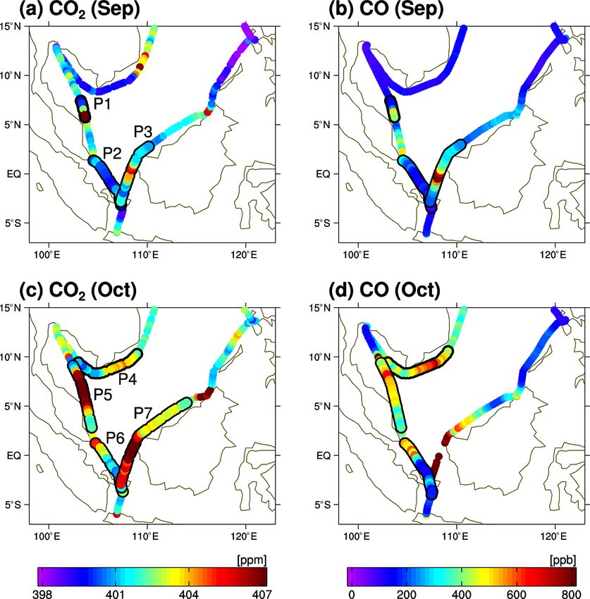
9458                             Y. Niwa et al.: Estimation of fire-induced carbon emissions from Equatorial Asia in 2015

where MT is the transpose of the tangent linear operator M
(in this study, Mδx ≈ M(δx) because of the linearity of the
problem). The MT calculation requires an adjoint model.
   The inversion system NISMON is specifically designed
for the inverse analysis of an atmospheric constituent (Niwa
et al., 2017a, b). In the system, the forward model of
NICAM-TM simulates atmospheric mole fractions from
given surface fluxes, and its adjoint model calculates the sen-
sitivities of fluxes against atmospheric mole fractions (Niwa
et al., 2017b). Specifically, the continuous adjoint model was
chosen for the adjoint calculation, assuring monotonicity of
tracer concentrations and sensitivities at the expense of mi-
nor nonlinearity (Niwa et al., 2017b). The optimisation cal-
culation uses the quasi-Newtonian algorithm of the Precon-
ditioned Optimizing Utility for Large-dimensional analyses        Figure 2. Schematic diagram of the CO2 –CO forward/adjoint cal-
(POpULar; Fujii and Kamachi, 2003; Fujii, 2005; Niwa et           culations in NICAM-TM.
al., 2017a).
   The atmospheric transport model NICAM-TM adopts an
                                                                  The atmospheric three-dimensional data of OH were derived
icosahedral grid system with hexagon- or pentagon-shaped
                                                                  from the TransCom-CH4 project (Spivakovsky et al., 2000;
grids (Fig. 1) that are produced by the recursive division of
                                                                  Patra et al., 2011). In the model, the contribution of oxidation
an icosahedron. All the model simulations were performed at
                                                                  from biogenic volatile organic compounds (BVOCs) to CO
a horizontal resolution of glevel-6 (n of glevel-n denotes the
                                                                  is not considered yet, but direct CO emissions from vegeta-
number of divisions of an icosahedron, representing the level
                                                                  tion are given at the Earth’s surface. Although the oxidations
of the model horizontal resolution). The averaged grid in-
                                                                  of CH4 and BVOCs are significant sources of atmospheric
terval of glevel-6 is 112 km, sufficiently resolving the major
                                                                  CO, we treated the former very simply and did not consider
archipelagos in Equatorial Asia (Fig. 1). For forward and ad-
                                                                  the latter. Therefore, we did not input CO observations to the
joint simulations of atmospheric transport, archived meteoro-
                                                                  inverse analysis. In the inversion, the biomass burning emis-
logical data drive NICAM-TM, which is an offline calcula-
                                                                  sions of CO, which were predominant in Equatorial Asia,
tion. The meteorological data were prepared in advance from
                                                                  were modified along with those of CO2 , as described in the
the simulation of the parent model NICAM, whose wind
                                                                  next section.
fields are nudged towards Japanese 55-year reanalysis data
(JRA-55; Kobayashi et al., 2015; Harada et al., 2016) (see        2.2.3   Flux model
Niwa et al., 2017b for a detailed description of the archived
meteorological data). Other model settings can be found in        As described in Fig. 2, we introduced scaling factors to sur-
Niwa et al. (2017b).                                              face fluxes, which is another updated feature of the inversion
                                                                  system from Niwa et al. (2017a). The surface CO2 flux input
2.2.2   Implementation of CO                                      to the model, fCO2 , is described as

In this study, we newly implemented a CO function in              fCO2 (x, t) = (1 + 1afos (x, t)) ffos (x, t)
the above inversion system to use CO as a proxy for fire-                    − (1 + 1aGPP (x, t)) fGPP (x, t)
induced emissions. It also considers oxidation from CO to
CO2 , which could have measurable effects on CO2 obser-                      + (1 + 1aRE (x, t)) fRE (x, t)
vations near fires. Figure 2 shows a schematic diagram for                   + (1 + 1afire (x, t)) ffire (x, t)
the forward and adjoint simulations of NICAM-TM, includ-                     + focn (x, t) + 1focn (x, t) ,                   (3)
ing CO. This CO function considers only the chemical reac-
tion with hydroxyl radicals (OH). The OH fields are given         where x and t indicate flux location and time, and f repre-
as input data; hence, the model does not have nonlinear           sents prescribed flux data, whose subscripts of fos, GPP, RE,
chemical reactions and thus retains its linearity, which is as-   fire and ocn denote flux components of fossil fuel combus-
sumed in the inverse analysis theory. Furthermore, the ox-        tion and cement production, gross primary production (GPP)
idation from methane (CH4 ) to CO with OH is also con-            and respiration (RE) of the terrestrial biosphere, biomass
sidered. For simplicity, however, the atmospheric mole frac-      burning and ocean, respectively. Note that a positive value
tion of CH4 was set at a globally constant value of 1844 ppb      indicates a flux towards the atmosphere. Each flux compo-
(= 10−9 mol−1 ), which was derived from the global an-            nent could have different temporal resolutions (e.g. monthly,
nual mean mole fraction for 2015, reported by the World           daily), and flux values are linearly interpolated in time to
Data Center for Greenhouse Gases (WDCGG; WMO, 2018).              each model time step. Datasets used for each flux component

Atmos. Chem. Phys., 21, 9455–9473, 2021                                             https://doi.org/10.5194/acp-21-9455-2021
Y. Niwa et al.: Estimation of fire-induced carbon emissions from Equatorial Asia in 2015                                      9459

are described in the following section. Their coefficients of       tion (Niwa et al., 2017a). Similarly, 80 % and 100 % errors
1afos , 1aGPP , 1aRE and 1afire are scaling factors for cor-        for fire emissions were introduced for Equatorial Asia and
responding flux components, of which the values could be            the rest of the world, respectively, but without spatial error
varied at each model grid. We did not apply the scaling fac-        correlations. Note that the fire errors for Equatorial Asia are
tor to the ocean flux but introduced the deviation of the pre-      practically larger than 80 %, because the 3 d temporal cor-
scribed flux 1focn because the ocean flux has both negative         relation inflates the errors. We put a 10 % error on the fos-
and positive values and its spatio-temporal flux phase could        sil fuel emissions in Equatorial Asia. For the monthly ocean
not be modified when introducing a scaling factor. Note that        flux errors, we used the standard deviation of the long-term
the other flux components should have all positive values.          data (1990–2016) and introduced a spatial error correlation
The phases of spatio-temporal variations of terrestrial bio-        of 3000 km. Table 1 shows each parameter.
sphere flux (e.g. seasonal cycle) could be modified because
GPP and RE are separately optimised. The above scaling fac-         2.2.5   Prescribed flux dataset
tors and 1focn were the parameters to be optimised in the
inverse analysis.                                                   For ffos and focn in Eq. (3), we used monthly mean data of
   For the surface CO flux, we considered fossil fuel, vegeta-      fossil fuel and cement production emissions from the Car-
tion and biomass burning emissions. For the biomass burning         bon Dioxide Information Analysis Center (CDIAC) (Andres
emissions, we imposed a common scaling factor with that of          et al., 2016) and of air–sea CO2 flux from the Japan Mete-
CO2 . Therefore, in the inversion, the biomass burning emis-        orological Agency (Takatani et al., 2014; Iida et al., 2015),
sions of CO was modified along with that of CO2 . The modi-         respectively. Here, the fossil fuel emissions data for 2015
fication of the biomass burning emissions could also be made        were produced from the latest gridded CDIAC data for 2013
by signals transported via atmospheric CO that should have          by scaling with the global total value for 2015 that is pre-
oxidised to CO2 (Fig. 2).                                           liminarily reported by Le Quéré et al. (2015). For fGPP and
   In Eq. (3), the temporal resolution of a flux-scaling fac-       fRE , we used 3-hourly data to resolve the distinct diurnal cy-
tor could be different from that of its corresponding flux and      cles of terrestrial biosphere flux. These fGPP and fRE were
be different by region (Table 1). In this study, we set a daily     originally based on monthly mean data from the Carnegie–
temporal resolution for the scaling factors of GPP, RE and          Ames–Stanford Approach (CASA) model (Randerson et al.,
biomass burning emissions in Equatorial Asia so that the in-        1997) but were modified according to the inversion of Niwa
version could exploit the full information of those surface         et al. (2012). They were further downscaled in time to 3-
fluxes from the observations. For the rest of the region, we        hourly with 2 m temperature and downward shortwave radi-
set monthly temporal resolutions. For the scaling factor of         ation data from JRA-55 using the method of Olsen and Ran-
fossil fuel emissions, we set an annual temporal resolution         derson (2004).
for Equatorial Asia, and we did not optimise the flux for the          In the inversion of Niwa et al. (2012), the classical low-
rest of the region, i.e. the modification factor was set to 0.      resolution inversion method (e.g. Enting, 2002) was used, in
We set a monthly temporal resolution for the deviation of the       which the global terrestrial area was divided into 31 regions,
ocean flux.                                                         and the scaling factors for those regions were optimised. Fur-
                                                                    thermore, the inversion used both surface and CONTRAIL
2.2.4   Error covariance matrices                                   data for 2006–2008, and the mean flux data of those three
                                                                    years were used in this study. Therefore, such an integrated
As in the case for the different flux temporal resolutions, we      flux could produce consistent atmospheric mole factions with
constructed the flux error covariance matrix B for Equato-          the observations from the surface to the upper troposphere,
rial Asia and the rest of the world separately. Table 1 sum-        although some discrepancies could arise because of the dif-
marises the standard errors and error correlations that were        ferent analysis period. In this study, these fluxes were op-
introduced into the diagonal and off-diagonal elements of           timised based on the CONTRAIL data from the study year
B, respectively. For GPP and RE, we assume 40 % error for           and further flux information was exploited using the 4D-Var
daily fluxes in Equatorial Asia and 10 % for monthly fluxes         high-resolution (model grid level) inversion with a specific
in the rest of the world, which means 0.16 and 0.01 for the         focus on Equatorial Asia.
diagonal elements of B. The higher standard error for Equa-            For the biomass burning flux of ffire , we used four datasets
torial Asia allows observations to modify surface fluxes suf-       and performed independent inversions to evaluate sensitivi-
ficiently. Nevertheless, a 3 d temporal error correlation was       ties to the biomass burning data (Table 2). The first is the
introduced to stabilise flux estimates. The smaller standard        mean of the GFED4s and GFAS v1.2 (noted as GG). The sec-
error for the rest of the world had to constrain the surface        ond and third are from GFED4s (GD) and GFAS v1.2 (GS),
flux to the prior because we did not use enough observations        respectively. The fourth is made by excluding emissions in
to cover the globe. Furthermore, for stabilisation, a spatial er-   Equatorial Asia from GG (NO). For NO, we replaced the
ror correlation length scale of 1000 km was introduced. The         biomass burning term of Eq. (3) by (0+1afire (x, t))ffire (x, t)
above error correlations were defined by the Gaussian func-         in Equatorial Asia, where ffire is the same as GG.

https://doi.org/10.5194/acp-21-9455-2021                                             Atmos. Chem. Phys., 21, 9455–9473, 2021
9460                                Y. Niwa et al.: Estimation of fire-induced carbon emissions from Equatorial Asia in 2015

Table 1. Temporal resolution, standard error and error correlation of each flux component, which were separately configured for Equatorial
Asia and the rest of the world. Note that the ocean flux was optimised by its absolute value and the others by their scaling factors; therefore,
the monthly standard deviation (SD) of the long-term data was used for the ocean flux error and ratios were used for the other flux errors. n/a
means not applicable.

                         Flux           Temporal resolution          Standard error     Error correlation (space/time)
                         component      Eq. Asia     Rest        Eq. Asia     Rest      Eq. Asia       Rest
                         fos            Annual       n/a         10 %         n/a       None/None      n/a
                         GPP, RE        Daily        Monthly     40 %         10 %      None/3 d       1000 km/None
                         fire           Daily        Monthly     80 %         100 %     None/3 d       None/None
                         ocn            n/a          Monthly     n/a          SD        n/a            3000 km

Table 2. Observation and prior fire-emission data for each inverse          where 1a and 1f ocn represent all the modification scal-
analysis experiment.                                                        ing factors and ocean flux deviations of Eq. (3), respec-
                                                                            tively, and 1c denotes the modification to the global offset.
  Experiment     Observation            Fire prior                          Thus, its corresponding basic state vector x 0 is described as
  name                                                                      x 0 = (1, . . ., 1, f ocn , 0)T . Note that the forward model calcu-
  C_GG           CONTRAIL               (GFAS + GFED) / 2                   lation started from a reasonable spatial gradient, which was
  C_GD           CONTRAIL               GFED                                prepared in advance by a spin-up calculation. At the begin-
  C_GS           CONTRAIL               GFAS                                ning of the 4D-Var iterative calculation, all the elements of
  C_NO           CONTRAIL               No fire in Equatorial Asia          δx were set to zero as the initial estimates.
  CV_GG          CONTRAIL, VOS          (GFAS + GFED) / 2                      The target period for this study is the whole year of 2015.
                                                                            However, in the inverse calculation, two extra months were
                                                                            added before the target period to attenuate the errors in the
                                                                            initial mole fraction fields before the beginning of 2015,
   For CO, the same biomass burning datasets from GFED4s                    which was inevitable because of the global unique parameter
and GFAS v1.2 were used. Note that both the datasets use                    described above (1c). Nevertheless, the initial mole fraction
similar emission factors of CO2 and CO based on Akagi et                    fields are consistent with observations to some extent, as they
al. (2011); in particular, the same emission factor from Chris-             were prepared by the inversion flux of Niwa et al. (2012).
tian et al. (2003) was applied to peatland, from which a large              This makes the two-month inversion spin-up reasonable. Fur-
part of the fires arise in Equatorial Asia (van der Werf et al.,            thermore, one more month was also added after the target pe-
2017). The rest of the CO fluxes from fossil fuel use and veg-              riod to well constrain the fluxes at the end of 2015. Therefore,
etation were derived from the Emission Database for Global                  the inverse calculation period consists of 15 months from
Atmospheric Research (EDGAR) version 4.3.2 (Janssens-                       November 2014 to January 2016.
Maenhout et al., 2019) and the process-based model of ter-
restrial ecosystems, the Vegetation Integrative SImulator for               2.3   Notation of sensitivity tests
Trace gases (VISIT; Ito and Inatomi, 2012; Ito, 2019), re-
spectively. In the VISIT simulation, CO emissions are es-                   As described in Sect. 2.2.5, we performed inversion analy-
timated with the scheme of Guenther (1997) but using an                     ses with four biomass burning datasets (GG, GD, GS and
emission factor by Tao and Jain (2005). The emission rates                  NO). We only used the CONTRAIL data, but with GG, we
are estimated by light, temperature, vegetation leaf amount                 additionally performed an inversion using the NIES VOS
and seasonality, and the scheme has been calibrated with ob-                data and CONTRAIL to leverage all available observations,
servational data. For EDGAR v4.3.2, we used emission data                   denoting C_ and CV_ as prefixes, respectively. Thus, we
from 2012 (the latest data available) for the simulation of                 have five inversion results (C_GG, C_GD, C_GS, C_NO and
2015.                                                                       CV_GG) (Table 2). Note that although they used different
                                                                            biomass burning data, prior flux errors for biomass burning
2.2.6   Initial mole fraction field and analysis period                     (Table 1) were commonly used. It is true even for C_NO
                                                                            whose practical prior uncertainty in Equatorial Asia is 80 %
In addition to the flux-scaling factors, the model parameter                of GG.
vector includes the global offset of atmospheric mole frac-
tions. Therefore, δx of Eqs. (1) and (2) is constructed as

                    T
δx = 1a, 1f ocn , 1c ,                                           (4)

Atmos. Chem. Phys., 21, 9455–9473, 2021                                                        https://doi.org/10.5194/acp-21-9455-2021
Y. Niwa et al.: Estimation of fire-induced carbon emissions from Equatorial Asia in 2015                                    9461

3     Results                                                     fire-induced CO tracers (the fire emissions of GG were used
                                                                  here), we found that the fires in Borneo and Sumatra con-
In this section, we first describe spatio-temporal features of    tributed almost every notable mole fraction elevation except
the CONTRAIL and NIES VOS observational data with sup-            for 17 September and 15–16 October, both of which might
plemental model analyses. Then, we show the inversion re-         be contributed by the fossil fuel emissions in Jakarta (Fig. 6).
sults and demonstrate their validity by comparing posterior       As highlighted by the grey shades in Fig. 6, seven of those
mole fractions of CO and CO2 with the NIES VOS data.              events contributed by the fires are designated by P1, P2, ...,
                                                                  P7 in this study. These events will be used for evaluating
3.1    Observational features                                     the inverse analysis, especially for fire-emission features, as
                                                                  described in Sect. 3.2.2. Note that mole fraction data from
As shown in Fig. 3, the CONTRAIL aircraft flew to Sin-            13–15 September and 11–14 October were excluded before
gapore 209 times during 2015. These high-frequency ob-            the analysis. During these periods, some data were not cor-
servations show a small but distinct seasonal cycle of CO2        rectly obtained because the signals were too large and out of
mole fractions around Equatorial Asia, with double peaks in       the measurable range. Furthermore, the NIES VOS ship trav-
April–May and December, and a minimum in June–October,            elled slowly or stayed around the Malacca Straits, resulting
depending on altitudes and latitudes. Furthermore, the CON-       in contamination by the ship’s own exhaust.
TRAIL aircraft frequently observed additional highly ele-            Figure 7 shows sensitivities of the CONTRAIL and NIES
vated mole fractions below 3 km altitude over Singapore           VOS observations against surface CO2 fluxes, i.e. footprints,
(Fig. 3a, lower panel), which could be attributable to local      for September and October 2015, calculated by the adjoint
or regional emissions in Equatorial Asia. The model with          model of NICAM-TM (Niwa et al., 2017b). The CON-
the prior flux data produced similar mole fraction eleva-         TRAIL footprints represent sensitivities of observations ob-
tions; however, their timing and magnitudes were sometimes        tained during ascending or descending flights over Singapore
different from the observations (Fig. 3b). A further model        (i.e. the data shown in the lower panel of Fig. 4a). For both
analysis with prior biomass burning data suggested that fire      September and October, the calculated footprints indicate
contributions to the observed mole fraction elevations were       that the CONTRAIL observations could provide significant
limited mostly to the latter period of the dry season from        constraints on flux estimates for Equatorial Asia, especially
mid-August to the beginning of November (Fig. 4b). Nev-           Borneo (Fig. 7a and b). These widespread footprint features
ertheless, a model simulation that separately calculated CO2      are because the data were obtained in the free troposphere,
mole fractions from other different sources (fossil fuel emis-    which is an advantage of aircraft observations in terms of
sions, terrestrial biosphere and ocean fluxes, and oxidation      representativeness. Figure 7 also suggests that the constraint
of CO) indicated that these fire contributions are dominant       is stronger during October than September because the num-
in the CO2 mole fraction variations over Singapore for this       ber of data is larger in October (Figs. 3 or 4). Compared to
period. In the other seasons, the model showed almost no          CONTRAIL, the NIES VOS footprints are restricted to the
contributions from fire emissions (not shown). In particular,     ocean (Fig. 7c and d) because the observations were made
the model showed a distinct fire contribution at the end of       within the marine boundary layer. Another contributing fac-
September, which elevated mole fractions up to the upper tro-     tor is the weak wind fields, which are typical in the tropics.
posphere by ∼ 4 ppm. In the observations, although similar        Nevertheless, there are some sensitivities of the NIES VOS
mole fraction elevations are found in the upper troposphere,      observations on the coasts of the islands, with which the sig-
its magnitude is smaller (∼ 2 ppm). Furthermore, the obser-       nificantly large fire emissions elevated the mole fractions of
vation shows a slightly later peak that lasted until the begin-   atmospheric CO2 and CO (Figs. 5 and 6).
ning of October (Fig. 4a). After that, the observations also
captured elevated mole fraction events from mid-October on-       3.2     Inversion results
ward. However, the prior model estimate showed smaller
fire contributions in October than in September (Fig. 4b),        3.2.1    Posterior fluxes
although the simulated total CO2 mole fractions were com-
parable to the observations (Fig. 3b), indicating that non-fire   In this study, we investigate surface fluxes by the sum of
emissions (e.g. from terrestrial biosphere respiration and fos-   CO2 and CO fluxes, defined as a carbon flux. Furthermore,
sil fuel emissions) had a certain level of contribution during    we evaluate the carbon flux separately for the total net flux
this period.                                                      and biomass burning emissions. Note that the total net flux
   Figure 5 shows CO2 and CO mole fractions observed              includes terrestrial biosphere fluxes, biomass burnings emis-
along the track of the NIES VOS around Equatorial Asia.           sions and fossil fuel emissions.
The NIES VOS observations in both September and Oc-                  Table 3 summarises the total net and fire carbon fluxes
tober 2015 captured coincident elevations of CO2 and CO           of Equatorial Asia estimated by the five sets of inversions.
mole fractions in the east of the Malay Peninsula and west        The prior biomass burning emissions of GG, GD and GS are
of Borneo. By performing a transport simulation of tagged         consistently 300 Tg C for September–October, which consti-

https://doi.org/10.5194/acp-21-9455-2021                                            Atmos. Chem. Phys., 21, 9455–9473, 2021
9462                                Y. Niwa et al.: Estimation of fire-induced carbon emissions from Equatorial Asia in 2015

Figure 3. CO2 mole fractions in the free troposphere around Equatorial Asia (note that data in the boundary layer and stratosphere are
excluded; see the main text) observed by CONTRAIL (a) and their corresponding prior (GG) (b) and posterior (C_GG) (c) model values
deviated from the observations. Each upper panel presents a time–latitude cross section from cruising mode data (∼ 11 km above sea level)
within the longitude range of 90–130◦ E and the lower panel shows a time–altitude cross section from ascending and descending data over
Singapore. Note that the data in the upper panels are not only from the Singapore flights but from all flights within the range. For the
visualisation, the data are all 5 d running means. Note also that an additional offset of 1.93 ppm is added to the prior mole fractions so that
the resulting global offset equals the posterior one. On the righthand side, correlation coefficients and root mean square difference (RMSD)
(ppm) between the simulated and observed mole fractions are noted for each time–latitude and time–altitude cross section.

tutes ∼ 80 % of the annual total fire emissions and amounts               September–October and all months in 2015, respectively.
to more than 80 % of the total net flux we prescribed as the              These numbers are in better agreement with the previous
prior (355–360 Tg C) for September–October. By inversion,                 top-down estimates of Huijnen et al. (2016) (227 Tg C for
all experiments, other than C_NO, estimated smaller total                 September–October and 289 Tg C for the annual total) and
net fluxes than prior data by ∼ 10 % (304–324 Tg C), and                  Heymann al. (2017) (204 Tg C for July–November) than that
they were mostly contributed by the smaller estimates of fire             of Yin et al. (2016) (510 Tg C for the annual total). Fur-
emissions (256–277 Tg C). Interestingly, even when prior fire             thermore, the fire-induced carbon emissions of 273 Tg C for
emissions were excluded in Equatorial Asia (C_NO), high                   September–October are also consistent with an aerosol-based
fire emissions of 122 Tg C were retrieved for September–                  study by Kiely et al. (2019), the best estimate of which is
October, indicating that the CONTRAIL data measure fire-                  247 Tg C as the sum of CO2 and CO emissions for Equa-
emission signals. However, the estimate is half of the others,            torial Asia but not including eastern areas (e.g. Papua New
indicating some dependency of the inversion on the prior fire             Guinea). Field et al. (2016) pointed out that the fire emis-
emissions.                                                                sions estimated by GFED for Equatorial Asia in 2015 are
   Our conceivably best estimate of CV_GG, which used                     higher than the annual fossil fuel emissions of Japan. Our es-
both the CONTRAIL and NIES VOS data, amounts to                           timate is smaller than that of GFED but still comparable to
273 and 362 Tg C for fire-induced carbon emissions from

Atmos. Chem. Phys., 21, 9455–9473, 2021                                                      https://doi.org/10.5194/acp-21-9455-2021
Y. Niwa et al.: Estimation of fire-induced carbon emissions from Equatorial Asia in 2015                                           9463

Figure 4. The same as Fig. 3, but for 15 August–15 November. The
model simulations here show only fire contributions.                Figure 6. Time series of CO mole fractions obtained by the in situ
                                                                    NIES VOS measurement (black) for September (a) and October (b)
                                                                    and corresponding simulation results by NICAM-TM with prior
                                                                    CO emissions data (red). These time series depict the data limited
                                                                    within the range of 95–125◦ E and 10◦ S–15◦ N consistently with
                                                                    Fig. 5b and d. Model simulations only from fire emissions in Suma-
                                                                    tra and Borneo are denoted by blue and cyan colours, respectively.
                                                                    Grey shades with P# indicate the fire-induced elevated mole fraction
                                                                    events.

                                                                    Table 3. Total net flux and fire emissions of carbon from Equatorial
                                                                    Asia for September–October 2015. Figure 1 defines the geograph-
                                                                    ical region of Equatorial Asia. Note that the total net flux includes
                                                                    terrestrial biosphere fluxes, biomass burnings emissions and fossil
                                                                    fuel emissions. Annual flux values for 2015 are also noted in paren-
                                                                    theses. The prior fluxes with the four biomass burning emissions are
                                                                    presented as well as the posterior fluxes of the five inversions.

                                                                                             Total net flux   Fire emissions
                                                                                                    (Tg C)           (Tg C)
                                                                               Prior (GG)        357 (677)         299 (388)
                                                                               Prior (GD)        360 (685)         301 (396)
                                                                               Prior (GS)        355 (669)         296 (379)
                                                                               Prior (NO)         59 (289)              0 (0)
Figure 5. Mole fractions of CO2 (a, c) and CO (b, d) along the                 C_GG              324 (613)         277 (363)
cruise tracks of NIES VOS for September (a, b) and October (c, d)              C_GD              304 (598)         256 (343)
2015. Data enclosed by black lines with P# represent designated                C_GS              320 (604)         265 (348)
fire-induced high mole fraction events (see also Fig. 6).                      C_NO              211 (451)         122 (131)
                                                                               CV_GG             322 (608)         273 (362)

the latest Japanese inventory (338 Tg C yr−1 for 2018; GIO
and MOE, 2020).                                                     of biomass burnings. However, the total emissions estimate is
   Figures 8 and 9 show the CO2 flux distributions for              smaller than the prior by 31 Tg (Fig. 8c). In October, the dif-
September and October, respectively. Here, we present the           ferences between prior and posterior fluxes of C_GG were
posterior fluxes of C_GG and C_NO only, but those of the            moderate, with a net difference of 2.7 Tg (Fig. 9c). In fact,
other inversions show similar distribution features to C_GG.        these flux changes are small compared with the differences
In September, C_GG estimated high emissions in Southeast            between GFED and GFAS (GFED minus GFAS is 92 and
Sumatra and south of Borneo, where the fire emissions dom-          −87 Tg C for September and October, respectively), indicat-
inated in the prior flux (Fig. 8), supporting prior knowledge       ing that the simulated mole fractions from the prior flux of

https://doi.org/10.5194/acp-21-9455-2021                                              Atmos. Chem. Phys., 21, 9455–9473, 2021
9464                               Y. Niwa et al.: Estimation of fire-induced carbon emissions from Equatorial Asia in 2015

Figure 7. Sensitivity of surface CO2 flux against the observations (e.g. footprints) of CONTRAIL over Singapore (a, b) and NIES VOS (c, d)
for September (a, c) and October (b, d) 2015.

Figure 8. Prior (a) and posterior (b: C_GG, e: C_NO) surface CO2 flux distributions averaged for September 2015. Differences between
prior and posterior fluxes (c, f) and prior fire emissions (d) are also shown. Note that the prior estimate of (a) was used both for C_GG and
C_NO, while the prior fire estimate of (d) was used only for C_GG.

Atmos. Chem. Phys., 21, 9455–9473, 2021                                                     https://doi.org/10.5194/acp-21-9455-2021
Y. Niwa et al.: Estimation of fire-induced carbon emissions from Equatorial Asia in 2015                                       9465

Figure 9. Same as Fig. 8, but for October 2015.

C_GG were overall consistent with the CONTRAIL obser-
vations.
   As shown in Table 3, even when the fire emissions were
excluded from the prior, the inversion estimated notable fire
emissions (C_NO) in both September and October (Figs. 8e
and 9e). Furthermore, the locations of the estimated fire
emissions are well coincident with those of prior fire emis-
sions in Southeast Sumatra and south of Borneo. They were
to some extent guided by the higher prior flux errors that were
derived from the fire-emission data (the uncertainty was set
as 80 % of GG), which was confirmed by another sensitivity
test without prior uncertainty of fire emissions (not shown).
Nevertheless, this result confirms that the CONTRAIL data
have information about biomass burning emissions.
   Figure 10 shows temporal variations of the total net carbon
flux in Equatorial Asia. Here, the posterior fluxes of C_GG
and CV_GG are shown (panel a) and the difference from
each prior is presented as 1 (panel b). Note that the time se-    Figure 10. Time series of posterior total net carbon fluxes (a) and
ries of 1 is smoother because 1 is the parameter optimised        their differences from prior (1) (b) for 2015. Posterior fluxes of
by the inversion with a 3 d temporal correlation scale. This      C_GG (blue) and CV_GG (red) and their prior flux (grey) are pre-
temporal correlation works as a smoother. The differences         sented.
between the two posterior fluxes are marginal, indicating a
limited effect of adding the NIES VOS data to the CON-
TRAIL data because the number of CONTRAIL data is over-              Figure 11 exhibits temporal variations of fire emissions
whelming and the footprint of CONTRAIL covers Equato-             during the fire season. In Equatorial Asia, although the tim-
rial Asia much more extensively in space (Fig. 7). Compared       ings of the emission peaks presented by GFED and GFAS are
to the prior flux, the posterior fluxes have a smaller peak at    coincident with each other, their magnitudes are significantly
the beginning of September, whereas they show larger peaks        different. GFED has larger peaks than GFAS in September,
from the end of September to the beginning of October. In         whereas it has smaller ones in October (Fig. 11a). Generally,
the latter part of October, the prior and posterior fluxes are    the posterior fire emissions, except for C_NO, fall within the
similar.                                                          range of both prior emission estimates. In September, the
                                                                  posterior estimates are consistent and their magnitudes are
                                                                  closer to GFAS than GFED. In October, however, notable

https://doi.org/10.5194/acp-21-9455-2021                                            Atmos. Chem. Phys., 21, 9455–9473, 2021
9466 Y. Niwa et al.: Estimation of fire-induced carbon emissions from Equatorial Asia in 2015
ulated for CONTRAIL have shown much better agreement
with the observations than the prior ones, demonstrating that
the inverse analyses were reasonably well performed. Com-
pared to the simulation results of the prior fluxes, the poste-
rior mole fractions have greater correlation coefficients and
smaller root mean square differences from the observations
(see the numbers at the righthand side of Fig. 3). In the fol-
lowing, we will compare the model with the CO2 and CO ob-
servations of NIES VOS, which were left independent of the
inversions, except for CV_GG. As demonstrated by Fig. 2,
the posterior CO flux includes the fire emissions modified
according to the modification of CO2 fire emissions. To elu-
cidate carbon fluxes in Equatorial Asia, the NIES VOS data
used here are limited in the neighbouring region (95–125◦ E
and 10◦ S–15◦ N).
In the comparative analysis of CO2 observations, an ad-
ditional offset of 1.93 ppm is added to the prior CO2 mole
fractions so that the resulting global offset becomes equiva-
lent to the posterior ones, i.e. 1c of Eq. (4) is 1.93 ppm (note
that there is almost no difference in the global offset among
Figure 11. Time series of posterior and prior fire carbon emissions the five inversions). Because the initial global offset was arbi-
over the fire season (mainly, September–October) of 2015. The pos-
trarily given, the comparison analysis of CO2 should exclude
terior fluxes of C_GG (blue solid), C_GD (orange solid), C_GS
the effect of the improvement in the global offset to better
(cyan solid) and C_NO (magenta solid) are shown. Prior data of
GFED (black dotted) and GFAS (grey dotted) are also shown. understand the inversion effects.
Figure 12 demonstrates how the posterior mole fractions
of CO2 and CO were improved from the prior ones. Compar-
discrepancies occur among the posterior emissions, which ing the posterior results with the prior ones, we found better
is contributed by different emission estimates for Sumatra consistency with the NIES VOS observation, which is true
rather than Borneo according to the breakdown of the poste- for both CO2 and CO. This is especially true for Septem-
rior estimates (Fig. 11b and c). In October, GFAS has higher ber; all inversions, except CV_GG, reduced the root mean
emissions than GFED on both islands and its degree is more square difference (RMSD) of CO2 from 2.14–2.62 to 2.05–
prominent in Sumatra. These different prior fire-emission 2.09 ppm, whereas those of CO were reduced from 92–211
estimates might have contributed to the large discrepancy to 80–111 ppb. These results indicate the validity of the in-
among posterior estimates. versions that used the CONTRAIL CO2 observations. Mean-
As shown in Fig. 7, the CONTRAIL footprint covers Bor- while, the RMSDs of both CO2 and CO were not necessar-
neo better than Sumatra, and the sensitivity is larger in Oc- ily reduced for October. This is attributable to insufficient
tober than in September. In practice, however, the constraint representativeness of surface fluxes or atmospheric transport,
on fire emissions has a different feature, as seen in the notice- which can be inferred from the larger RMSDs and the smaller
able spread of fire-emission estimates in October (Fig. 11c). correlations in October than those of September. Neverthe-
Note that the spread of estimates, including C_NO, is small less, the experiment without the prior fire emissions (C_NO)
in Sumatra at the end of September (Fig. 11b). In this pe- exhibited smaller RMSDs with the posterior CO2 and CO
riod, the observational data and model analysis indicated that fluxes for both September and October. Furthermore, the im-
strong fire signals reached Singapore, although its timing, as provement in the correlation coefficients is remarkable (in
suggested by the model, was slightly earlier (Fig. 4b). For September from 0.43 to 0.56 for CO2 and from 0.34 to 0.81
this event, the inversion successfully optimised the fire emis- for CO, whereas in October from 0.29 to 0.49 for CO2 and
sions in Sumatra with strong constraints by the observations, from −0.18 to 0.49 for CO). The other inversions, except for
even from the no-fire prior (C_NO), resulting in the later- CV_GG, did not improve the correlation coefficients signif-
shifted peak with the consistent magnitude of 4–5 Tg C d−1 icantly. In both months, CV_GG showed the best scores for
(Fig. 11b). CO2 , which is reasonable because it used the CO2 observa-
tions of NIES VOS. Note, however, that CV_GG used only
3.2.2 Posterior mole fractions the CO2 observations but not those of CO. Therefore, the
RMSD reduction of CO for September by CV_GG (from 136
In this section, we evaluate the simulated atmospheric CO2 to 103 ppb) demonstrates some improvement in fire emis-
and CO mole fractions from the posterior fluxes. First, as sions. Therefore, it is better to use both the CONTRAIL and
shown in Fig. 3, the posterior mole fractions of CO2 sim- NIES VOS observations for flux estimations; however, the
Atmos. Chem. Phys., 21, 9455–9473, 2021 https://doi.org/10.5194/acp-21-9455-2021Y. Niwa et al.: Estimation of fire-induced carbon emissions from Equatorial Asia in 2015 9467
Figure 12. Correlation coefficient (a, b) and root mean square difference (RMSD) (c, d) between the observed and simulated NIES VOS
CO2 (a, c) and CO (b, d) mole fractions. The NIES VOS data used here are limited within the range of 95–125◦ E and 10◦ S–15◦ N for
September (light blue) and October (light green) 2015. The model simulations are derived from each posterior flux (C_GG, C_GD, C_GS,
C_NO and CV_GG) (filled bar) and its corresponding prior flux (open bar). To consider the initial global offset error, we added 1.93 ppm to
every prior value so that the prior initial global offset becomes equivalent to the posterior one.
impact of NIES VOS is limited for the total carbon fluxes in
Equatorial Asia (Table 3 and Fig. 10).
For each elevated mole fraction event defined by Figs. 5
and 6, we calculated an enhancement ratio of 1CO / 1CO2
from the reduced major axis regression, as done by Nara et
al. (2017). For all peaks, except P1 and P2, every correla-
tion between CO2 and CO variations is statistically signif-
icant (p < 0.05) for both the observations and simulations.
For P1 and P2, some simulated results could not have signif-
icant correlations; therefore, we combined the two events so
that every correlation was statistically significant (combin-
ing P1 and P2 would be reasonable because the Sumatra fires
contributed to both; see Fig. 6). The enhancement ratios for
those events could provide implications for emission ratios
between CO and CO2 . Note that the simulated ratios are de- Figure 13. Observed and simulated enhancement ratios of
rived from the posterior fluxes, but the overall feature does 1CO / 1CO2 (solid line) and observed correlation coefficients be-
not change when the prior fluxes are used because the fire- tween 1CO and 1CO2 (grey bar) for each elevated mole fraction
event defined by Figs. 5 and 6. The observed enhancement ratios
emission ratios between CO and CO2 were unchanged by
are coloured in black. The simulated values were derived from pos-
the inversion. Figure 13 depicts the observed and simulated terior CO and CO2 fluxes of C_GG (magenta), C_GD (red), C_GS
enhancement ratios and the observed correlation coefficients (blue), C_NO (green) and CV_GG (cyan).
for each event. The figure shows that the observed ratio has a
significantly large variation from 0.034 to 0.169 ppb ppb−1 .
Interestingly, the higher ratios were obtained from events that the simulated ratios have substantial spreads among the dif-
were likely contributed to by the Borneo fires (P3, P6 and P7; ferent inversions, especially for P6 (0.080–0.145 ppb ppb−1 )
see also Fig. 6). The model reproduced a pattern similar to and P7 (0.123–0.182 ppb ppb−1 ), and the observed ratios are
the observed one. However, for the events from September to almost at the highest level of the simulated spreads. This is
early October (P1 and P2, P3 and P4), the model coherently discussed further in the following section.
overestimated the enhancement ratios. The model and obser-
vations, respectively, show 0.067–0.104 and 0.038 ppb ppb−1
for P1 and P2, 0.139–0.165 and 0.117 ppb ppb−1 for P3, and
0.115–0.133 and 0.066 ppb ppb−1 for P4. In the latter events,
https://doi.org/10.5194/acp-21-9455-2021 Atmos. Chem. Phys., 21, 9455–9473, 20219468 Y. Niwa et al.: Estimation of fire-induced carbon emissions from Equatorial Asia in 2015
4 Discussion biomass burnings from other terrestrial fluxes. To separate
fire-induced and other terrestrial fluxes, it would be helpful
This study used high-precision in situ observations of CO2 to to incorporate CO observations simultaneously with CO2 ob-
estimate carbon fluxes in contrast to studies that used satel- servations into the inverse analysis; however, the availability
lite observations of CO (Huijnen et al., 2016; Yin et al., of in situ CO observations (Novelli et al., 2003) is limited,
2016). Therefore, we obtained the total net carbon flux that especially for Equatorial Asia. A joint CO2 –CO inversion is
included biomass burning emissions, terrestrial biosphere left for a future study.
photosynthesis and respiration, and fossil fuel emissions. The second limitation is the dependency of the inverse
The estimated total net carbon flux amounts to 322 Tg C analysis results on the prior estimate. We found that our in-
for September–October (CV_GG), 85 % of which is con- verse calculations had a significant sensitivity to prior fire-
tributed by fire emissions (Table 3), indicating that flux vari- emission data. The posterior fluxes were similar when GFED
ations of terrestrial photosynthesis and respiration under se- or GFAS data were used as the prior. However, when the
vere drought were not as large as those of the biomass burn- prior fire emissions were excluded (i.e. C_NO), the poste-
ing emissions in 2015. This result indicates that biomass rior flux had much lower values, indicating that we can-
burning emissions are the main driving force of interannual not fully constrain the fluxes with CONTRAIL alone and
variations of carbon fluxes in Equatorial Asia, which is a that prior fire-emission data should be as accurate as possi-
unique feature of the carbon fluxes in this region compared ble. The relatively small sensitivity to the difference between
with other tropical regions. Carbon fluxes in the tropics are GFED and GFAS was because the original GFED and GFAS
considered to have significant sensitivities to climate vari- data are comparable. Nevertheless, the well-constrained flux
ations, especially to El Niño, with major driving forces of at the end of September in Sumatra (Fig. 11) tells us that
terrestrial biosphere flux changes in response to temperature we could obtain a sufficient constraint from CONTRAIL
and precipitation changes (Yang and Wang, 2000; Zeng et when the time and location of the observations coincide with
al., 2005; Wang et al., 2013). the timing of airflow rich in emission signals. Such an air-
As described in Sect. 2.2, we used a common scaling fac- flow dependency could be reduced by making the observa-
tor for CO2 and CO fire fluxes; therefore, the ratio of the tions denser in space and time. To this end, the CONTRAIL
emission factors (CO / CO2 ) was fixed to that of prior fire- project continues its efforts to improve data coverage.
emission data (GFED and GFAS) and burned carbon mass Finally, model transport errors would be the third limita-
was modified by the inverse analysis. It is likely that the tion. Figures 3 and 4 show that even after the inversion, the
spatial pattern of fire-emission ratios was reasonably repre- model could not sufficiently reproduce high mole fractions
sented because the model reproduced the observed variation near the surface, suggesting some limitation of the model.
in the enhancement ratio that might be caused by the differ- Compared to the wind data obtained from the CONTRAIL
ence in their origins (Figs. 6 and 13). However, as shown aircraft, the speed and direction of winds over Singapore
in Fig. 13, the model overestimated the enhancement ratios were well simulated in the model (not shown). Therefore,
from September to early October, irrespective of its origin representative errors that include both model transport and
(Borneo or Sumatra). Meanwhile, it was not the case for the fluxes could be one cause. A higher resolution model is de-
latter period, although the simulated ranges were large, in- sirable and is left for a future study with advanced computa-
dicating that the temporal change of the fire-emission ratio, tional resources.
i.e. a decrease of combustion efficiency, might not be well In this study, we tried a regionally focused inversion us-
represented in the fire-emission data. Typical fire-emission ing different flux parameter settings for Equatorial Asia and
ratios of CO / CO2 are 0.2–0.3 mol mol−1 for peatlands and the rest of the world (Table 1), which gave a sufficient de-
0.1 mol mol−1 for tropical forests, respectively (Akagi et al., gree of freedom to fluxes in Equatorial Asia, while strongly
2011; Huijnen et al., 2016; Stockwell et al., 2014). There- constraining fluxes to the prior ones in the rest of the world.
fore, the observed smaller enhancement ratio infers that the This inversion approach would be acceptable only when prior
contribution of fires (or smouldering) in dried peatlands was fluxes can produce comparable spatio-temporal variations of
smaller in the early fire period than expected. This might atmospheric CO2 with observations, which was confirmed
have partially resulted in the smaller-than-prior estimates of using the previous inversion flux of Niwa et al. (2012). Fur-
the fire-induced carbon emissions (Table 3) because peat- thermore, Niwa et al. (2012) found that CONTRAIL data
lands have a high carbon density and are dominant sources could independently constrain the fluxes in Equatorial Asia
of carbon (Page et al., 2002). Nevertheless, the uncertainty itself, supporting the validity of separating fluxes in Equato-
is high, as demonstrated by the large model spreads, espe- rial Asia from those in the other regions. Nevertheless, the
cially for the latter period, and we need more observations inversion flux used as the prior in this study was optimised
for robust estimations of the fire-emission ratio. for different years, which introduced a certain level of uncer-
We noted that the inverse analysis of this study has sev- tainty. In a future analysis, an effort for reducing uncertain-
eral limitations. First, we employed only CO2 observations in ties will be made by performing a global inverse analysis by
the inverse analysis, which does not allow us to distinguish combining ground-based stations and CONTRAIL data.
Atmos. Chem. Phys., 21, 9455–9473, 2021 https://doi.org/10.5194/acp-21-9455-2021You can also read