The Atlantic's freshwater budget under climate change in the Community Earth System Model with strongly eddying oceans
←
→
Page content transcription
If your browser does not render page correctly, please read the page content below
Ocean Sci., 17, 729–754, 2021
https://doi.org/10.5194/os-17-729-2021
© Author(s) 2021. This work is distributed under
the Creative Commons Attribution 4.0 License.

The Atlantic’s freshwater budget under climate change in the
Community Earth System Model with strongly eddying oceans
André Jüling, Xun Zhang, Daniele Castellana, Anna S. von der Heydt, and Henk A. Dijkstra
Institute for Marine and Atmospheric research Utrecht (IMAU), Utrecht University, Utrecht, the Netherlands

Correspondence: André Jüling (a.juling@uu.nl)

Received: 23 July 2020 – Discussion started: 18 August 2020
Revised: 15 January 2021 – Accepted: 2 February 2021 – Published: 28 May 2021

Abstract. We investigate the freshwater budget of the At-           tion carries about 1.5 PW of heat northwards at 26.5◦ N in the
lantic and Arctic oceans in coupled climate change simula-          Atlantic (Johns et al., 2011), and hence its strength and spa-
tions with the Community Earth System Model and compare             tial expression significantly affect local surface temperature
a strongly eddying setup with 0.1◦ ocean grid spacing to a          and precipitation (Palter, 2015). The potential tipping char-
non-eddying 1◦ configuration typical of Coupled Model In-           acter of the AMOC is expressed through large and abrupt
tercomparison Project phase 6 (CMIP6) models. Details of            changes in AMOC strength (Srokosz et al., 2012; Weijer
this budget are important to understand the evolution of the        et al., 2019), for which evidence exists in the palaeo record
Atlantic Meridional Overturning Circulation (AMOC) under            (Lynch-Stieglitz, 2017). In models of the AMOC, such tran-
climate change. We find that the slowdown of the AMOC               sitions can occur due to the existence of multiple equilibria,
in the year 2100 under the increasing CO2 concentrations of         where several AMOC states can coexist under the same forc-
the Representative Concentration Pathway 8.5 (RCP8.5) sce-          ing conditions. Such multiple equilibria of the AMOC have
nario is almost identical between both simulations. Also, the       been found in a hierarchy of ocean–climate models (Stom-
surface freshwater fluxes are similar in their mean and trend       mel, 1961; Rahmstorf et al., 2005; Hawkins et al., 2011;
under climate change in both simulations. While the basin-          Toom et al., 2012; Mecking et al., 2016). They occur due
scale total freshwater transport is similar between the simu-       to the presence of positive feedbacks, the most prominent
lations, significant local differences exist. The high-ocean-       one being the salt advection feedback (Peltier and Vettoretti,
resolution simulation exhibits significantly reduced ocean          2014). Subtle changes to the freshwater budget can modify
state biases, notably in the salt distribution, due to an im-       the AMOC response to perturbations which is why the cor-
proved circulation. Mesoscale eddies contribute considerably        rect simulation of the oceanic freshwater budget in the Arctic
to the freshwater and salt transport, in particular at the bound-   and Atlantic is important (Behrens et al., 2013).
aries of the subtropical and subpolar gyres. Both simulations          The Atlantic is a net evaporative basin resulting in the
start in the single equilibrium AMOC regime according to            saltiest subtropical surface waters of all the major oceans. At
a commonly used AMOC stability indicator and evolve to-             the Atlantic’s southern boundary, which we take to coincide
wards the multiple equilibrium regime under climate change,         with the southern tip of Africa at 34◦ S, relatively salty sur-
but only the high-resolution simulation enters it due to the re-    face waters together with fresh Antarctic Intermediate Wa-
duced biases in the freshwater budget.                              ter (AAIW) are imported in the upper 1000 m. This north-
                                                                    ward transport amounts to approximately 17 Sv at 26.5◦ N
                                                                    (Moat et al., 2020; Smeed et al., 2018; Frajka-Williams et al.,
                                                                    2019). At high northern latitudes, the surface waters are
1   Introduction                                                    transformed into North Atlantic Deep Water (NADW) which
                                                                    returns southwards and is exported at 34◦ S. A lower, weaker
One of the important tipping elements in the climate system         overturning cell exists in which cold Antarctic Bottom Wa-
(Lenton et al., 2008) is the Atlantic Meridional Overturning        ter enters the South Atlantic at the bottom and returns just
Circulation (AMOC). This component of the ocean circula-

Published by Copernicus Publications on behalf of the European Geosciences Union.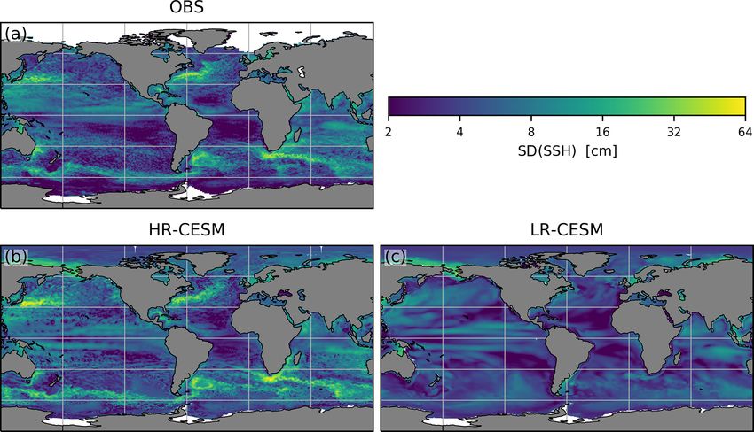
730                                                 A. Jüling et al.: The Atlantic’s freshwater budget under climate change

above with the NADW. Salt also enters the South Atlantic          and detail the computations of the different transport com-
from the southwest Indian Ocean via Agulhas leakage in the        ponents in Appendix B. Positive FovS values indicate that
form of eddies shed off the Agulhas retroflection (McDon-         the AMOC imports freshwater which constitutes a negative
agh et al., 1999). From the north, approximately 0.8 Sv of        feedback as a positive AMOC strength perturbation would
relatively fresh Pacific water enters the Arctic Ocean via the    be damped by an enhanced freshwater import into the North
Bering Strait where it further freshens primarily due to river    Atlantic, suppressing deep water formation. A negative FovS
discharge from the large Arctic catchment area (Woodgate          value, on the other hand, would induce an amplification of an
and Aagaard, 2005). Together with freshwater in the form of       AMOC perturbation (Huisman et al., 2010). Observational
sea ice, relatively fresh seawater enters the Atlantic from the   estimates of FovS are negative suggesting multiple AMOC
north. In the Strait of Gibraltar, relatively fresh surface wa-   equilibria in the present-day climate (Weijer et al., 2019).
ters flow into the strongly evaporative Mediterranean Sea and     The models of CMIP3 and CMIP5 tend to have positive FovS
saltier waters return into the Atlantic at depth. The merid-      values due to a salinity bias at 34◦ S, where the upper wa-
ional asymmetry of the precipitation pattern of the Intertrop-    ter masses are too fresh and the deep southward return flow
ical Convergence Zone (ITCZ) results in salinity differences      is too salty (Drijfhout et al., 2011; Weaver et al., 2012; Liu
between the North and South Atlantic. The wind-driven sub-        et al., 2014; Mecking et al., 2017). Once this bias is ac-
tropical and subpolar gyres recirculate water primarily hor-      counted for, FovS values for most models lie within the range
izontally and advect any zonal salinity gradient also in the      of observations (Mecking et al., 2017). Under increasing ra-
meridional direction.                                             diative forcing, CMIP3 models exhibit a negative FovS trend
   As atmospheric temperatures rise under increasing green-       (Drijfhout et al., 2011), but no consistent sign in this trend is
house gas concentrations, the hydrological cycle generally        found in CMIP5 models (Weaver et al., 2012).
strengthens, making dry regions drier and wet regions wet-           Refining the grid spacing from 1◦ typical of CMIP5 and
ter, amplifying sea surface salinity patterns (Held and So-       CMIP6 ocean model components to 0.1◦ resolves the internal
den, 2006; Skliris et al., 2020). The AMOC is projected to        Rossby radius of deformation over large parts of the ocean
weaken under climate change due to buoyancy flux changes          (Hallberg, 2013). This enables the development of eddies,
as heat flux and net precipitation patterns change (Stocker       filaments, and fronts through mixed barotropic/baroclinic in-
et al., 2013). The heat flux changes are the dominant driver      stabilities and the simulation of other mesoscale ocean fea-
of AMOC strength reduction, and there is evidence that this       tures such as currents at the western boundary and through
slowdown is already underway (Gregory et al., 2005; Cae-          narrow straits. We use the terminology “strongly eddying”
sar et al., 2018). In order to judge how fast the AMOC can        for ocean grids with 0.1◦ horizontal grid spacing as these
change and whether it could collapse abruptly, one needs to       are neither just eddy-permitting (typically 0.25◦ ) nor fully
assess the AMOC stability and in particular the strength of       mesoscale turbulence resolving (Moreton et al., 2020). These
the positive feedbacks. In Coupled Model Intercomparison          high-resolution ocean models constitute the only consistent
Project phase 5 (CMIP5) models, no transition to a different      method to estimate eddy contributions to ocean variability
statistical equilibrium state is found up to the year 2100 un-    and the mean climate state and generally result in signif-
der any of the climate change scenarios (Cheng et al., 2013),     icantly reduced ocean biases (Kirtman et al., 2012; Small
and it remains unclear whether the AMOC is already in or          et al., 2014). The eddy freshwater transport is comparable in
will shift into a multiple equilibrium regime, which would        magnitude to the mean transport at the poleward and equa-
allow such transitions (Gent, 2018).                              torward boundaries of the subtropical gyres (Treguier et al.,
   Many studies have linked the freshwater budget, through        2012, 2014). Some of this transport will be captured by eddy
the salt advection feedback, to the response of the AMOC          parameterizations in low-resolution simulation, but other ef-
under surface freshwater perturbations (Rahmstorf, 1996;          fects, such as the advection of salt by Agulhas rings, cannot
de Vries, 2005; Dijkstra, 2007; Mecking et al., 2017; Liu         be captured adequately.
et al., 2017). The existence of a multiple equilibrium regime        Relatively few studies have investigated the AMOC be-
is connected to the sign of the divergence of the advective       havior in strongly eddying ocean models (Weijer et al.,
AMOC induced Atlantic freshwater transport 6 (or 1Mov in          2012; den Toom et al., 2014; Brunnabend and Dijkstra,
Liu et al., 2017) which exactly marks the separation of the       2017; Hirschi et al., 2020). The improved simulation of over-
unique and multiple equilibrium regimes when atmospheric          flows over sills in high-resolution models significantly re-
feedbacks are negligible (Dijkstra, 2007). As the northern        duces deep water density biases which leads to improved
boundary freshwater transport is minor, this divergence is of-    simulation of deep convection. The pathway of the North
ten approximated by its southern boundary component only,         Atlantic Current and the formation sites of North Atlantic
referred to as Mov (de Vries, 2005), Fov (Hawkins et al.,         Deep Water are more realistic at high resolution (Hirschi
2011), or FovS (Weijer et al., 2019). We will use FovS here       et al., 2020). A comparison of the AMOC response between
as we use F to denote freshwater fluxes in general and Fov        10 Geophysical Fluid Dynamics Laboratory (GFDL) mod-
for the latitudinally dependent overturning component in par-     els under a 1 % yr−1 CO2 increase scenario showed that in
ticular. We define freshwater relative to a salinity of S0 = 35   coarse-resolution models, the AMOC declines between 16 %

Ocean Sci., 17, 729–754, 2021                                                          https://doi.org/10.5194/os-17-729-2021
A. Jüling et al.: The Atlantic’s freshwater budget under climate change                                                      731

and 45 %, and the eddy-permitting and strongly eddying con-       face freshwater fluxes are thus modeled as virtual salt fluxes.
figurations are at the lower end of these percentages with        The high-resolution (“HR”) simulation was performed with
13 % and 16 %, respectively (Winton et al., 2014). The POP        a 0.1◦ ocean horizontal grid spacing on a tripolar grid, while
ocean model showed qualitatively similar AMOC responses           the low-resolution (“LR”) simulation was conducted with 1◦
to surface freshwater perturbations between strongly eddy-        ocean horizontal grid spacing with a displaced dipole grid.
ing (0.1◦ ) and non-eddying (1◦ ) model configurations (Wei-      Tracer diffusing subgrid-scale processes are parameterized
jer et al., 2012; den Toom et al., 2014; Brunnabend and Di-       by the Gent–McWilliams scheme (Gent and McWilliams,
jkstra, 2017) but with a dependence on the location of the        1990) in the 1◦ simulation and by biharmonic diffusion in
perturbation. However, whether ocean model resolution af-         the 0.1◦ case, which is strongly eddying.
fects the AMOC response to forcing systematically remains            Both control simulations use constant year-2000 atmo-
an open question (Gent, 2018), although there is evidence         spheric greenhouse gas concentrations forcing (notably
from eddy-permitting models that the AMOC mean state,             [CO2 ] = 367 ppm, [CH4 ] = 1760 ppb). The HR-CESM sim-
in particular the sites of deep water formation, controls the     ulation continues from a National Center for Atmospheric
response (Jackson et al., 2020). A suite of high-resolution       Research (NCAR) simulation of several decades which itself
ocean-only hindcasts with the Nucleus for European Mod-           was initialized from a motionless ocean with a present-day
elling of the Ocean (NEMO) model at 1/12◦ show that the           estimate of the ocean’s temperature and salinity distribution.
stability indicator FovS is negative (Deshayes et al., 2013) in   The LR-CESM simulation was similarly continued from an
contrast to coarse-resolution coupled models (Mecking et al.,     NCAR-provided initial state. The climate change simulations
2017). The NEMO model thus shows a reduced bias in FovS ,         are following the CO2 concentration of the highest Represen-
but it remains unclear how much of the bias reduction is due      tative Concentration Pathway (RCP8.5) of CMIP5 used in
to the use of restoring boundary conditions within the ocean-     the Fifth Assessment Report of the Intergovernmental Panel
only setup and how much is due to an improved mean state          on Climate Change (Stocker et al., 2013) but do not in-
of the ocean circulation.                                         clude other greenhouse gas increases or land use changes.
   As coarse-resolution models exhibit biases in their mean       We name the present-day control simulation CTRL and the
state and lack mesoscale processes, the simulated sensitiv-       climate change simulation RCP. In 2100, the radiative forc-
ity to forcing may be inadequate and the strength of the salt     ing of CO2 alone is 6.9 W m−2 , or 80 % of the 8.5 W m−2
advection feedback may be affected. We investigate the ef-        of the RCP8.5 scenario (van Vuuren et al., 2011). Not pre-
fect of improving the ocean model resolution on the Atlantic      scribing land use changes has no effect on the global mean
freshwater budget and its sensitivity by analyzing present-       surface temperature in the RCP8.5 scenario (Davies-Barnard
day control and high-CO2 concentration pathway simula-            et al., 2014). Compared to the mean warming in 2100 of
tions in two configurations of the Community Earth System         the two RCP8.5 CESM1/CAM5 simulations submitted to
Model: one with an ocean model grid spacing of 0.1◦ and           CMIP5 at 4.4 ◦ C (Meehl et al., 2013; time series avail-
the other with 1◦ . The following section (Sect. 2) describes     able at https://climexp.knmi.nl/CMIP5/Tglobal/, last access:
these model simulations and provides a model–observation          30 April 2021), our LR-CESM RCP simulation warmed only
comparison of the control simulations. Section 3 presents the     2.9 ◦ C, or 66 % of the RCP8.5 value. The reduced warming
results, including changes to the AMOC, the Atlantic fresh-       until 2100 is both because of the aforementioned reduced ra-
water and salt budgets, and the effects on AMOC stability,        diative forcing but also because our simulation started from
under the climate change scenario. The results are summa-         a nearly equilibrated, and hence relatively warm, year-2000
rized and discussed in Sect. 4.                                   control simulation. The main characteristics of the model
                                                                  simulations are summarized in Table 1.
                                                                     There are additional differences between the model con-
2     Model simulations and model–observation                     figurations apart from the horizontal ocean model resolution.
      comparison                                                  The 0.1◦ POP2 model grid has 42 levels to 6000 m, while
                                                                  the LR-POP2 grid has 60 levels to 5500 m. In contrast to
2.1    CESM simulations                                           the HR-CESM ocean grid with its partial bottom cells and
                                                                  explicitly resolved overflows, the LR-CESM grid is defined
We analyze four simulations with the Community Earth Sys-         with complete bottom cells and uses overflow parameteriza-
tem Model version 1 (CESM1; Hurrell et al., 2013), car-           tions, e.g., between the Nordic Seas and the Atlantic (Smith
ried out at the Academic Computing Center in Amsterdam            et al., 2010). In the 0.1◦ POP2 model, the explicitly mod-
(SURFsara); see, e.g., van Westen and Dijkstra (2017). The        eled Nordic Seas overflows compare favorably to observa-
CESM components are CAM5 (Community Atmosphere                    tions (Ypma et al., 2019). The Mediterranean outflow is not
Model version 5), POP2 (Parallel Ocean Program 2), CICE           parameterized in the 1◦ POP2 grid but is modeled with a
(Los Alamos Sea Ice Model), and CLM (Community Land               widened Strait of Gibraltar. Ultimately, the effect of the dif-
Model), which are coupled by the CESM1 coupler. The               ferent vertical resolutions is hard to disentangle as the hor-
ocean model formulation is volume conserving, and sur-            izontal mixing is represented very differently. Further, the

https://doi.org/10.5194/os-17-729-2021                                                          Ocean Sci., 17, 729–754, 2021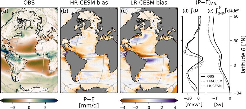
732 A. Jüling et al.: The Atlantic’s freshwater budget under climate change
Table 1. Overview of the CESM simulations used, their ocean and atmosphere grid, and the model version, as well as the year at which the
RCP simulations are branched off the CTRL simulations.
Setup Ocean grid Atmosphere grid CESM version Start of RCP [year]
HR-CESM 0.1◦ tripole, 42 levels to 6000 m tx0.1v2 0.47◦ ×0.63◦ f05 1.0.4 200
LR-CESM 1◦ dipole, 60 levels to 5500 m gx1v6 0.9◦ ×1.25◦ f09 1.1.2 500
CESM versions and atmosphere resolution differ between perature dataset (HadISST) 1990–2019 climatology (Rayner
the HR-CESM (version 1.0.4) and the LR-CESM simula- et al., 2003), the bias of the CTRL simulations with respect
tions (version 1.1.2). The newer version employs a differ- to that climatology, and the linear SST trends of the RCP
ent dynamical core in the atmosphere model (CAM5.2 ver- simulations. The HR-CESM (LR-CESM) simulation global
sus CAM5.0), and some parameterization schemes are up- mean SST is about 0.51(0.86) K too warm with a RMSE of
dated. In contrast to the improvement in ocean model reso- 0.99(1.39) K compared to the HadISST dataset. Some warm
lution, however, halving the atmospheric grid spacing from bias is to be expected as the simulations are subjected to con-
1 to 0.5◦ is not resolving new essential physical processes. stant year-2000 radiative forcing and not the transiently in-
Therefore, no significant changes are expected between the creasing historical forcing. In the HR-CESM Atlantic, the sea
0.5◦ CAM5.0 HR-CESM and 1◦ CAM5.2 LR-CESM sim- surface is slightly too cold equatorward of 30◦ and too warm
ulations’ atmospheres due their resolved physics apart from poleward of these latitudes with the exception of the South
coupling to different ocean boundary conditions. Atlantic near the African coast. The LR-CESM SST biases
are stronger with warm biases in the South Atlantic, along the
2.2 Model–observation comparison North American east coast due to the Gulf Stream separating
too far north, and north of 50◦ N. The LR-CESM NA-STG
To assess the performance of the HR- and LR-CESM CTRL and the southern edge of the NA-SPG are too cold result-
simulations, we use several observational datasets which ing in asymmetric bias around the Equator. Both simulations
are relevant for the freshwater budget and compare 30-year SSTs are too high in the NADW formation areas which re-
means of the CTRL simulations following the RCP branch- sults in warm biases in this water mass. The RCP SST trends
off point (years 200–229 and 500–529; see Table 1). In many are positive everywhere with a marked Arctic amplification.
aspects the HR-CESM CTRL simulation performs better The exception is the NA-SPG with negative SST trends, an
than the LR-CESM CTRL simulation when compared to the expected response associated with an AMOC decline under
present-day climate. Global maps of the quantities presented radiative forcing (Drijfhout et al., 2012).
here for the Atlantic–Arctic are included in Appendix A.
When linear fits are presented, such as in Fig. 1d and e, sig- 2.2.2 Surface freshwater fluxes
nificance of the fit is tested with a Wald test against a zero-
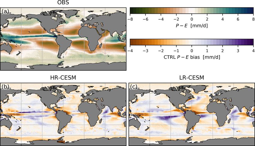
slope null hypothesis. We compare surface freshwater fluxes to the ERA-Interim
We define regions in the Atlantic that approximately cor- precipitation minus evaporation, P –E, 1989–2010 climatol-
respond to the subtropical gyres (STGs; sometimes speci- ogy (Dee et al., 2011; Trenberth et al., 2011). Figure 2 shows
fied as South or North Atlantic: SA-STG and NA-STG), the maps of the observed mean P –E and the bias of the two
subpolar gyre (SPG), the ITCZ, and the Arctic. Green lines simulations, and the zonally integrated P –E fluxes. There
in Fig. 1b and c show bounding latitudes which are at the is net evaporation in the STGs and net precipitation in the
southern end of the Atlantic basin around 34◦ S, 10◦ S, and ITCZ just north of the Equator (Fig. 2a) and the midlati-
10◦ N generously bounding the ITCZ, 45◦ N as the approx- tudes to high latitudes. Both simulations exhibit the same
imate boundary of the subtropical and subpolar gyres, and positive global precipitation biases of 0.23 ± 1.01 mm d−1
60◦ N as the boundary between the Atlantic and the Arctic. (mean ± RMSE; see Appendix A). The P –E bias is nega-
The Arctic Ocean includes Hudson Bay and is bounded on tive almost everywhere in the HR-CESM Atlantic (Fig. 2b)
the Pacific side by the Bering Strait at 68◦ N. We perform the and over large parts of the LR-CESM Atlantic (Fig. 2c). Both
calculations on the original model 0.1 and 1◦ grids which be- simulations show biases around the ITCZ, most noticeably
come distorted relative to a regular latitude–longitude grid at with reduced precipitation near the South American coast
high northern latitudes (see 60◦ N line in Fig. 1). north of the Equator. The HR-CESM ITCZ appears slightly
rotated with a wider precipitation belt in the central equato-
2.2.1 Sea surface temperature rial Atlantic and reduced precipitation in the northwest and
southeast. The LR-CESM ITCZ is shifted south because the
The sea surface temperature (SST) is important for the fresh- SST bias (see Fig. 1c) is meridionally asymmetric around
water budget as it strongly controls evaporation. Figure 1 the Equator. As the surface waters diverge at the Equator
shows the Hadley Centre Sea Ice and Sea Surface Tem- this contributes to the saline (fresh) surface bias of the North
Ocean Sci., 17, 729–754, 2021 https://doi.org/10.5194/os-17-729-2021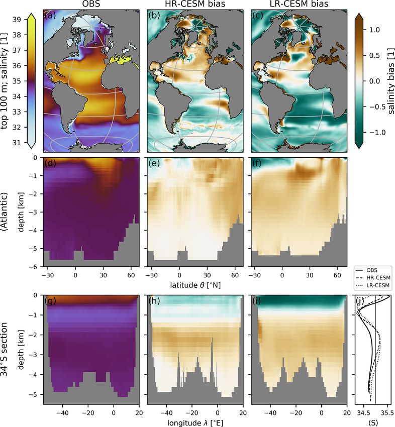
A. Jüling et al.: The Atlantic’s freshwater budget under climate change                                                                 733

Figure 1. The sea surface temperature (SST) from the HadISST 1990–2019 observations (a), the SST bias of the HR-CESM (b) and LR-
CESM (c) CTRL simulations, and the linear trends of the HR-CESM (d) and LR-CESM (e) RCP climate change scenarios. Hatched areas
in the trend maps are not significant at the 5 % level. The Lambert azimuthal projection of these and subsequent maps is an equal-area
projection, and gray parallels (meridians) are drawn every 30◦ (60◦ ). The green lines (b, c) show transects in the tripolar 0.1◦ and dipolar
1◦ POP2 model grid at 34, 10◦ S, 10◦ N, and approximately 45 and 60◦ N. This northernmost meridional boundary differs from the 60◦ N
parallel because of the curvilinear grids and is chosen to lie south of the Hudson Strait.

Figure 2. Precipitation minus evaporation: the observed ERA-Interim 1980–2010 climatology (a) and the biases of the HR-CESM (b) and
LR-CESM (c) CTRL simulations. The zonally integrated P –E fluxes per degree latitude (d) and the implied freshwater transport due to the
P –E fluxes (e) assuming zero transport at 34◦ S and constant salt content in the oceans. Note that this does not include runoff freshwater
contributions.

(South) Atlantic. Around the Gulf Stream too much water                  vations averaged over 1990–2019 which are provided on a
evaporates, but this is stronger and extends further north in            1◦ × 1◦ grid (Good et al., 2013). To compare to the model
the LR-CESM simulation, reflecting SST biases there (see                 data, we first interpolated the EN4 data bilinearly horizon-
Fig. 1c). Both the flux per degree latitude and the merid-               tally and then linearly to the model depth coordinates for
ionally integrated flux referenced to zero transport at 34◦ S            both HR- and LR-CESM ocean grids. Figure 3 shows the ob-
shown in Fig. 2d and e reveal comparable biases in the zonal             served salinity distribution and the simulation biases of the
integrals with minor differences in the ITCZ.                            upper 100 m, as an Atlantic zonal mean, and along a zonal
                                                                         transect at 34◦ S. Both HR-CESM (Fig. 3b) and LR-CESM
2.2.3   Salinity distribution                                            (Fig. 3c) show a similar bias pattern with a positive surface
                                                                         bias in the North Atlantic and parts of the Arctic, and a nega-
The heterogeneous salinity distribution in the ocean is the              tive bias in the South Atlantic and the rest of the global ocean
result of surface exchanges of freshwater and redistribution             (Appendix Fig. A3). The Atlantic zonally averaged profile
by the circulation. We use the EN4 global salinity obser-

https://doi.org/10.5194/os-17-729-2021                                                                    Ocean Sci., 17, 729–754, 2021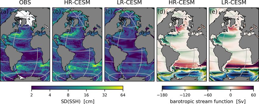
734                                                      A. Jüling et al.: The Atlantic’s freshwater budget under climate change

Figure 3. The salinity distribution in the EN4 observations (a, d, g) and the bias of the HR-CESM (b, e, h) and LR-CESM (c, f, i) CTRL
simulations for the top 100 m (a, b, c), zonally averaged in the Atlantic (d, e, f), and at the 34◦ S transect (g, h, i). Panel (j) shows zonally
averaged salinity profiles for observations (thick solid line) and the HR-CESM (dashed) and LR-CESM (dotted) simulations together with
the reference salinity S0 = 35 (thin solid). Note that salinity as a mass fraction is dimensionless.

(Fig. 3d) shows the largest salinity values in the evapora-                2.2.4    Circulation and gateway transport
tive subtropical gyres with less saline waters of the NADW
with S = 34.9–35.0 at high northern latitudes and between                  In Fig. 4a, b, and c, we compare the standard deviation of the
1500 and 4000 m, while relatively fresh AAIW is visible                    observed sea surface height (SSH; Zlotnicki et al., 2019) and
around 1000 m depth up to 10◦ N. The AAIW is visible in the                the modeled dynamic sea level to illustrate the fidelity of the
34◦ S transect (Fig. 3g) and the section average (Fig. 3j). The            HR-CESM simulation. The SSH observations are provided
bias in HR-CESM is significantly reduced compared the LR-                  as 5 d means on a 1/6◦ grid, and some polar data are missing.
CESM simulation in all three planes. In particular, the LR-                For Fig. 4a, we use the year 2018 to calculate the standard de-
CESM simulation bias around 1000 m depth and 15–30◦ N                      viation from the 5 d means. In Fig. 4b and c, we calculate the
(Fig. 3f) can be attributed to the absence of eddies (Treguier             standard deviation for the branch-off year of the CTRL sim-
et al., 2014).                                                             ulations based on the SSH2 and SSH output variables. This
                                                                           means that the modeled dynamic sea level standard deviation
                                                                           uses the model time step as the sampling frequency, in effect
                                                                           capturing more variability than the 5 d sampling of the ob-
                                                                           servations. The observations and model are thus not directly

Ocean Sci., 17, 729–754, 2021                                                                     https://doi.org/10.5194/os-17-729-2021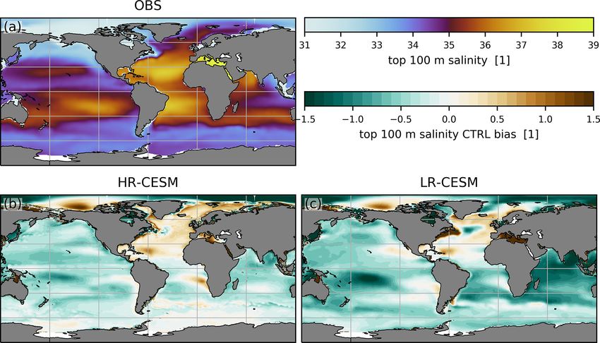
A. Jüling et al.: The Atlantic’s freshwater budget under climate change                                                            735

Figure 4. (a) The standard deviation of the observed sea surface height anomalies on a 1/6◦ grid (Zlotnicki et al., 2019). Missing data
are white. (c, d) The dynamic sea level standard deviation of the HR- and LR-CESM CTRL simulations. (d, e) The mean barotropic
streamfunction 9 of the HR- and LR-CESM CTRL simulations relative to the African Atlantic coast.

comparable in all details, but the LR-CESM clearly lacks               ocean water parcel. We choose S0 = 35, as this is the salinity
variability compared to the observations and HR-CESM, in               of the modeled North Atlantic Deep Water and close to the
particular in regions of the Gulf Stream and its extension, the        average salinity at 34◦ S (see Figs. 3d, g, and j). In principle,
Agulhas retroflection, the Argentine Basin, and the Antarctic          the freshwater framework has disadvantages, as the choice
Circumpolar Current.                                                   of the reference salinity S0 is arbitrary and the amount of
    To explain several of the HR- and LR-CESM salin-                   freshwater depends non-linearly on it (Schauer and Losch,
ity distribution biases, we plot the barotropic streamfunc-            2019). However, the relevant terms relate to recirculating and
tion for both CTRL cases in Fig. 4d and e. We ap-                      eddy flows which are independent of S0 (see Appendix B),
proximate
R θ R 0 the barotropic           streamfunction 9 as 9(λ, θ ) =        and the AMOC stability criterion FovS is framed in terms
             u(λ, θ 0 , z) dz dθ 0 − 9 . Here, the vertical integral   of freshwater. Only the barotropic transport depends on S0 ,
   0
  θ =θS z=D                           0
of the zonal velocity u is taken over the full depth from z = D        and this component is negligible for the Atlantic freshwater
to the surface z = 0, the meridional integral is taken from            transport although it contributes significantly to the total salt
the southern boundary at Antarctica (θ = θS ) and is subse-            transport.
quently set to 0 at the African Atlantic coast by removing a              For the Atlantic–Arctic basin the only oceanic exchanges
constant 90 . In LR-CESM, the barotropic streamfunction is             of freshwater and salt north of 34◦ S occurs at Bering Strait
diagnosed and part of the model output and this field agrees           with the Pacific Ocean and through the Strait of Gibraltar
well with our approximation. For consistency, we present our           with the Mediterranean Sea. Table 2 summarizes the ob-
approximation for both HR- and LR-CESM.                                served and simulated transport of seawater, salt, and freshwa-
    While the broad-scale wind-driven subtropical and sub-             ter. The Mediterranean is a net evaporative basin with a small
polar gyre circulation are present in both simulations, HR-            net volume inflow at the Strait of Gibraltar but an overturning
CESM features stronger boundary currents, standing ed-                 that is about 20 times stronger, importing waters with a salin-
dies, a more realistic Agulhas retroflection pathway and Gulf          ity of 36.2 and exporting Mediterranean Overflow Water at a
Stream separation point, and a stronger subpolar gyre which            salinity of 38.4 at a depth of 1000 m (Sánchez-Román et al.,
extends much further south along the North American coast.             2009). In reality, there is no source of salt in the Mediter-
In LR-CESM, the inflow of Indian Ocean waters is unrealis-             ranean, but as the model formulation is volume conserving,
tically strong and together with the strong upper 100 m fresh          there is no net flow through the Strait of Gibraltar and the
bias of the Indian Ocean (Appendix Fig. A3) contributes to             net evaporation in the model Mediterranean represents a vir-
the negative salinity bias of the South Atlantic (Fig. 3). In the      tual salt source. An overturning of 0.8 Sv with the aforemen-
RCP scenario, the Gulf Stream in HR-CESM shifts north-                 tioned salinity differences would result in a salt transport of
ward, which is expected under climate change (Yang et al.,             1.8 kt s−1 into the Atlantic. The model salt transport of both
2020). In LR-CESM, the subpolar gyre weakens broadly,                  simulations is somewhat smaller at 1.2 ± 0.1 kt s−1 , which is
while in HR-CESM only the boundary currents weaken (not                equivalent to a freshwater transport of 32 ± 2 mSv. Through
shown).                                                                the shallow Bering Strait, relatively fresh water with mean
    The freshwater fraction W , which we call freshwater for           salinity of 32.5 ± 0.3 flows northward into the Arctic Ocean
brevity, is defined relative to a reference salinity S0 as W =         because of dynamic sea level differences between the Arctic
(S−S0 )/S0 , where S is the (dimensionless) salinity of a given        and North Pacific (Woodgate and Aagaard, 2005).

https://doi.org/10.5194/os-17-729-2021                                                                Ocean Sci., 17, 729–754, 2021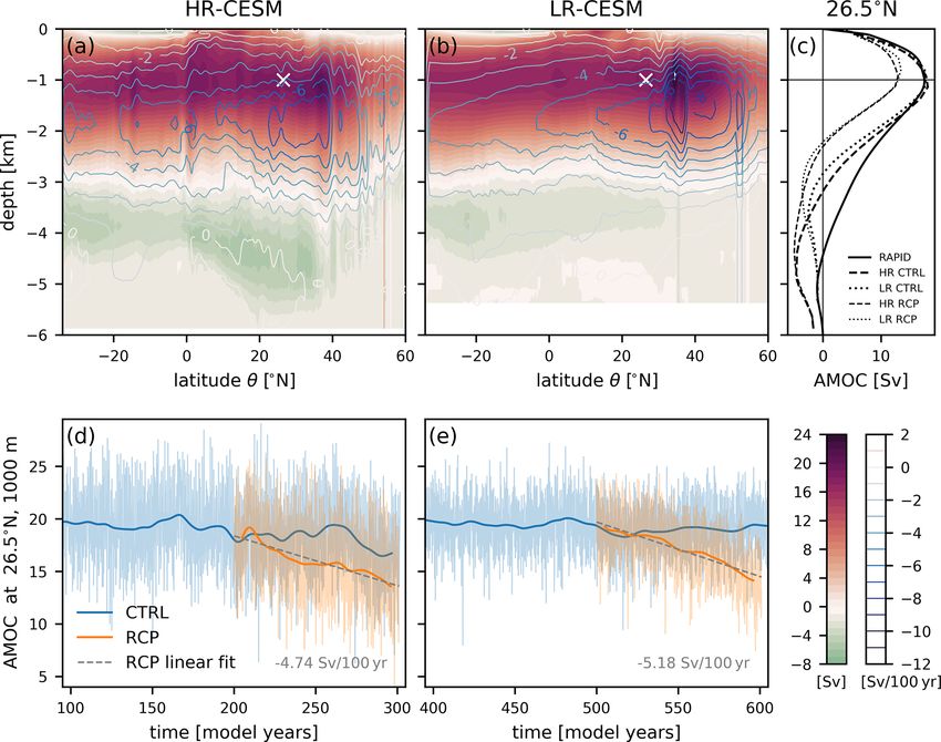
736                                                        A. Jüling et al.: The Atlantic’s freshwater budget under climate change

Table 2. Transport into the Atlantic of seawater, salt, and freshwater through the Bering Strait (Woodgate and Aagaard, 2005), the Strait of
Gibraltar (Sánchez-Román et al., 2009), and across 24◦ S (Bryden et al., 2011). The barotropic seawater volume transport Fbt        V is given for all
                                                        V                                                ◦
three transects and the overturning volume transport Fov is given for the Strait of Gibraltar and at 24 S. The mean salt transport Fmean  S    across
a section is defined as the integrated product of monthly salinity and velocity fields (the unit [kt s−1 ] is equivalent to the also commonly used
[Sv psu]). The mean freshwater transport Fmean is defined similarly with the reference salinity S0 = 35. The freshwater transport overturning
component Fov is given only at 24◦ S. The ± denotes uncertainties in the observations and interannual standard deviations in the simulations.
The two values for the observations at 24◦ S are estimates from two separate cruises.

                                 Transect     Term      Units                   OBS      HR-CESM         LR-CESM
                                 Bering        V
                                              Fbt       [Sv]                0.8 ± 0.1      1.6 ± 0.1       1.0 ± 0.1
                                               S
                                              Fmean     [kt s−1 ]              26 ± 3         51 ± 4          32 ± 1
                                              Fmean     [mSv]               140 ± 20       100 ± 30        100 ± 30
                                 Gibraltar     V
                                              Fbt       [mSv]                −38 ± 7           0±4             0±3
                                               V
                                              Fov       [mSv]                    800       430 ± 31        300 ± 25
                                               S
                                              Fmean     [kt s−1 ]                  0       1.1 ± 0.2       1.1 ± 0.1
                                              Fmean     [mSv]                   −50        −32 ± 2         −32 ± 2
                                 24◦ S         V
                                              Fbt       [Sv]        −0.755, −0.630       −1.6 ± 0.1      −1.0 ± 0.1
                                               V
                                              Fov       [Sv]                  21.5       17.0 ± 0.8      16.4 ± 0.7
                                               S
                                              Fmean     [kt s−1 ]             +0.3        −67 ± 5         −47 ± 3
                                              Fmean     [mSv]           −2.9, −2.4        290 ± 13        340 ± 14
                                              Fov       [mSv]           −130, −90         160 ± 10        270 ± 10

   Table 2 also lists the transport terms at 24◦ S as Bryden                 the Northern Hemisphere compared to the LR-CESM simu-
et al. (2011) provide Fov estimates from two cruises at this                 lation.
latitude. The simulated barotropic volume transport at 24◦ S                    The evolution of the AMOC strength is measured at the
equals that through the Bering Strait, because the model is                  latitude of the RAPID mooring array, 26.5◦ N, and the depth
volume conserving. The corresponding virtual salt flux for-                  of maximum overturning, 1000 m (white crosses in Fig. 5a
mulation is also the reason why the simulated mean salt                      and b). In contrast to the RAPID array data, the streamfunc-
transport is very negative, while observations show a small                  tion in Fig. 5c contains negligible contributions from the Gulf
northward salt transport. Both simulations’ overturning cir-                 of Mexico at 26.5◦ N. Figure 5d and e show time series of
culations are weaker than observed, and the freshwater trans-                the AMOC strength, including 100 years prior to the RCP
port due to the overturning is of opposite sign compared to                  branch-off point to show the statistically equilibrated nature
the observations.                                                            of the time series. Both simulations’ CTRL mean AMOC
                                                                             strength compare favorably to the observations with approxi-
                                                                             mately 18 Sv (Frajka-Williams et al., 2019), and they respond
                                                                             with a similar linear weakening trend of 4.7 Sv per century
3     Results                                                                and 5.2 Sv per century to the RCP forcing, respectively. The
                                                                             monthly variability (thin line) of HR-CESM is larger than in
3.1    AMOC                                                                  LR-CESM due to the presence of an eddying ocean.

Figure 5a and b show the AMOC streamfunction ψ(θ, z)                         3.2    Surface freshwater fluxes
of the CTRL mean state (shading) together with the RCP
trends (contours) in both HR- and LR-CESM. The maximum                       The Atlantic is a net evaporative basin, and Fig. 6 shows
of ψ is located just below 1000 m depth for both simula-                     maps of the total surface freshwater flux, Fsurf , and its major
tions around 35◦ N, but the LR-CESM simulation upper cell                    contributing components: precipitation (P ) and evaporation
stretches further north consistent with its STG that extends                 (E). In addition, Fsurf comprises runoff from land R and ice,
too far north (see Fig. 4). The Antarctic Bottom Water cell is               as well as sea ice melt (brine rejection) which, from here on,
stronger and extends further north in HR-CESM. Both sim-                     are all defined as positive (negative) freshwater fluxes into
ulations experience a similar weakening and shoaling trend                   the ocean. Precipitation occurs mainly in the ITCZ region
of the upper cell and a slight strengthening of the lower cell.              (with stronger maxima in HR-CESM), over the Gulf Stream,
The HR-CESM latitudinal gradient in the weakening trend                      and in the midlatitude storm tracks. In the HR-CESM (LR-
around the maxima at 2000 m is weaker so that the HR-                        CESM) CTRL simulation between 34◦ S and 60◦ N, there is a
CESM AMOC weakening is stronger at 34◦ S but weaker in                       net freshwater loss of 0.85(0.93) Sv which is relatively large

Ocean Sci., 17, 729–754, 2021                                                                        https://doi.org/10.5194/os-17-729-2021
A. Jüling et al.: The Atlantic’s freshwater budget under climate change 737
Figure 5. AMOC mean streamfunctions ψ(θ, z) of the HR-CESM (a) and LR-CESM (b) CTRL simulations together with the linear trends
as contour lines every 1 Sv per century. At 26.5◦ N and 1000 m depth, the white crosses mark the location of AMOC strength whose
time evolution is depicted in panels (d) and (e). Panel (c) compares the modeled CTRL mean streamfunction profiles at 26.5◦ N (thick
dashed/dotted) to the RAPID observations (solid) and also presents the changed streamfunction after 100 years in the RCP simulation (thin
dashed/dotted). Monthly (thin) and 10-year low-pass-filtered (thick) AMOC time series of the HR-CESM (d) and LR-CESM (e) CTRL
(blue) and RCP (orange) simulations. The linear trends are indicated by dashed gray lines and their values are written in the lower right.
compared to the CMIP5 freshwater loss (e.g., 0.48 ± 0.13 Sv between the simulations include smaller positive trends along
in the historical multi-model mean in Fig. 6 of Skliris et al., the US east coast due to the different Gulf Stream separation
2020). Evaporation is strongly tied to SSTs (cf. Figs. 1a, b, c behavior and the related southward extent of the subpolar
and 6e, f) with most occurring in the subtropical gyres and at gyre. The runoff into the Atlantic and Arctic increases al-
the above-zonal-average SSTs of the western boundary cur- most everywhere with the exception of Amazon basin rivers.
rents and their extensions. Runoff occurs from all coasts bor- In the polar regions, changing freshwater input from melting
dering the Atlantic and is artificially distributed over larger sea ice is locally significant, e.g., east of Greenland where
areas surrounding the river mouths in the model which is vis- the total freshwater trends (Fig. 6c, d) are more negative than
ible in the total freshwater flux subplots of Fig. 6. the evaporative component alone would suggest (Fig. 6g, h)
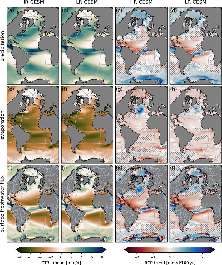
The forced freshwater flux trends in Fig. 6 reveal the gen- despite increases in precipitation (Fig. 6c, d) due to higher
eral intensification of the hydrological cycle as SSTs gener- atmospheric temperatures. The trends of the surface fresh-
ally increase (Fig. 1d, e). Total surface freshwater flux linear water flux components are similar on a large scale between
trends of −0.14(−0.16) Sv per century between 34◦ S and HR-CESM and LR-CESM (see Fig. 9).
60◦ N (see Fig. 9a) in the HR-CESM (LR-CESM) RCP sim-
ulation intensify the Atlantic’s evaporative nature. The no- 3.3 Meridional transport of freshwater
table exception to this global trend in both simulations is the
subpolar gyre where SSTs decline, which results in less evap-
We decompose the meridional freshwater transport into dif-
oration and hence a larger net freshwater flux into the ocean.
ferent terms related to the overturning and azonal gyre cir-
This reduction in evaporation in the SPG is more pronounced
culation as well as an eddy component (equations in Ap-
in HR-CESM compared to LR-CESM. Regional differences
pendix B). Budget term computations are performed on the
https://doi.org/10.5194/os-17-729-2021 Ocean Sci., 17, 729–754, 2021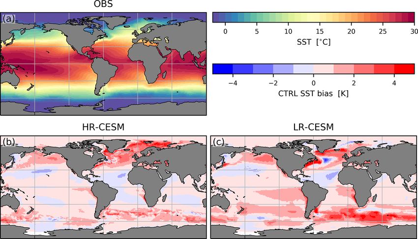
738                                                     A. Jüling et al.: The Atlantic’s freshwater budget under climate change

Figure 6. The major freshwater flux components, precipitation P (a–d) and evaporation E (e–h), and the total freshwater flux Fsurf (i–l). The
means of the HR-CESM (a, e, i) and LR-CESM (b, f, j) CTRL simulations and the linear trends of the HR-CESM (c, g, k) and LR-CESM (d,
h, l) RCP simulations. Polygons near river mouths in panels (i)–(l) are areas where runoff is distributed by the ocean model. Hatched areas
in the trend maps are not significant at the 5 % level.

original ocean model grid which leads to small differences               ues of the linear RCP trends (top row), as well as the trends
between model zonal transects and the true parallel of a given           themselves (bottom row).
latitude in the midlatitudes to high latitudes of the Northern              At 60◦ N, the total freshwater transport Ftot (red lines in
Hemisphere (green lines in Fig. 1b and c). Figure 7 shows                Fig. 7) is negative because relatively fresh water is imported
the meridional dependence of the different zonally integrated            via the Bering Strait into the Arctic where it further fresh-
northward freshwater transport components. The figure in-                ens mostly due to runoff (Table 2). Despite different volume
cludes both the 30-year CTRL means and the year-2100 val-                fluxes at Bering Strait, the freshwater inflow is about the
                                                                         same between the simulations at 0.10 ± 0.03 Sv because of

Ocean Sci., 17, 729–754, 2021                                                                  https://doi.org/10.5194/os-17-729-2021
A. Jüling et al.: The Atlantic’s freshwater budget under climate change 739
Figure 7. The meridional freshwater transport as a function of latitude θ for the HR-CESM (a, c) and LR-CESM (b, d) simulations. In
panels (a) and (b), solid lines are the means of the 30 CTRL years following the branch-off point and dashed lines are the year-2100 values
of the linear RCP fit. The total transport terms (red) are decomposed into an overturning (blue), an azonal gyre (orange), and an eddy
contribution (green). Panels (c) and (d) show the linear trends separately. Significant trends (at the 5 % level) are thick, while insignificant
trends are only thin. Vertical bars to the right of the panels illustrate the Arctic surface flux in the Arctic (purple) and the Bering Strait inflow
(olive) of freshwater.
the stronger fresh bias of the LR-CESM simulation (cf. Ta- biased ITCZ position of LR-CESM. In the following, we take
ble 2, Bering Strait salinity bias in Fig. 3b and c, and vertical a closer look at these two differences.
lines in Fig. 7). The Arctic is a net precipitative basin, in part The AMOC carries both relatively salty surface waters
due to its extensive catchment area, resulting in even more and fresh Antarctic Intermediate Water northward and salty
freshwater entering the Atlantic at 60◦ N. In the subpolar North Atlantic Deep Water south. The overturning freshwa-
gyre and the ITCZ, i.e., in latitudes of net precipitation, fresh- ter transport Fov (blue lines in Fig. 7) thus depends on the
water diverges (i.e., ∂Ftotal /∂θ > 0), while net evaporation in vertical distribution of the zonally averaged salinities rela-
the subtropical gyres results in freshwater convergence by the tive to the depth of the overturning cell (cf. Figs. 3 and 5).
oceanic transport. Under the RCP forcing scenario, the total Without changes to salinity, a weakening AMOC would re-
freshwater flow is more southward because more freshwater duce the overturning transport, and with a constant AMOC,
enters at 60◦ N primarily due to increased net precipitation the intensifying hydrological cycle would lead to enhanced
(including runoff) in the Arctic. Generally, meridional gra- meridional gradients in the transport across precipitative and
dients of the total transport in precipitative and evaporative evaporative parts of the ocean. With the weakening AMOC
latitudes increase as a result of the enhanced hydrological under the RCP scenario, the Fov trend is negative everywhere
cycle. Notable differences between the HR- and LR-CESM in LR-CESM, while the HR-CESM Fov trend is not latitu-
Ftot are at the STG–SPG boundary at 45◦ N, where the LR- dinally coherent in its sign. The HR-CESM Fov decrease
CESM Ftot does not exhibit the negative transport trend of around 40–50◦ N is caused by the northward migration of the
the HR-CESM Ftot and the meridional position of the tropi- boundary between the subtropical and subpolar gyres. The
cal freshwater transport divergence related to the southward- decrease in the overturning transport has some of its largest
expression at 34◦ S, and the salinity stratification bias of the
https://doi.org/10.5194/os-17-729-2021 Ocean Sci., 17, 729–754, 2021740 A. Jüling et al.: The Atlantic’s freshwater budget under climate change
South Atlantic (Fig. 3j) results in a positive FovS bias which CESM freshwater divergence contributes to the salinity bias
is more pronounced in LR-CESM compared to HR-CESM. (see Fig. 3f).
In the absence of eddies, the decomposition of the total
flow into the overturning and azonal component depends on 3.4 Salinity trends
the azonal nature of the velocity and salinity fields. Both the
North and South Atlantic subtropical gyres transport fresh- In the RCP climate change scenario, the Atlantic’s salinity
water north (orange lines in Fig. 7) due to their opposite changes significantly as surface freshwater fluxes and trans-
zonal asymmetry in salt content near the surface where the port convergences change, even though these salt storage
majority of horizontal gyre transport takes place (Fig. 3), changes are small compared to the fluxes and their changes.
while the subpolar gyre transports freshwater south. Bound- Figure 8 shows the linear trend of the vertically averaged
ary currents, which comprise an important part of the azonal salt content for the surface (0–100 m) and subsurface (100–
flow, are better resolved in the HR-CESM simulation (cf. 1000 m) layers. In the forced salinity response, the signature
Figs. 1, 2, 3, and 4). Under the climate change scenario, of the enhanced hydrological cycle is imprinted: the upper
the azonal freshwater transport term Faz generally becomes 1000 m of the Atlantic south of 45◦ N largely salinifies, in
more southward north of 20◦ S in the STGs and the SPG. The particular in the NA-STG. The freshening of the NA-SPG is
gyre transport trends consist both of a gyre strength signal also a consequence of the weakening AMOC and the asso-
(approximately the barotropic streamfunction of Fig. 4) and ciated warming hole (Menary and Wood, 2018). The surface
one due to the azonal salinity trend (Fig. 8). The HR-CESM subpolar gyre freshens uniformly in the LR-CESM simula-
Faz trends are the largest contribution to the total southward tion, but the subsurface shows largely insignificant trends. In
freshwater trends. In fact, between 20–40◦ N, the HR-CESM HR-CESM, only the eastern SPG freshens down to 1000 m
Faz trend is so negative due to the strong salinification along but salinifies in the East and West Greenland as well as
the North American Atlantic coast (Fig. 8) that the Fov trend Labrador currents bringing salt into the western SPG. This
becomes slightly positive (but not significantly so). This oc- is the result of advection of salinifying waters from the cen-
curs also around 5–20◦ S in the HR-CESM simulation where tral Arctic north of Greenland and Svalbard. While the Arc-
Faz switches signs under forcing. These negative Faz trends tic surface layer between the Bering Strait and the North Pole
are much weaker in LR-CESM so that the overturning com- becomes fresher in both simulations due to enhanced net pre-
ponent trend remains latitudinally coherent in its sign. cipitation including runoff (Fig. 6), the subsurface salinifies
Eddy transport of freshwater Feddy (green lines in Fig. 7) strongly in HR-CESM enhancing stratification. In the South-
is not associated with volume fluxes as they are due to corre- ern Hemisphere, enhanced runoff from Africa decreases the
lations between salinity and flow anomalies, which we define salinity in the eastern SA-STG, whereas decreasing runoff
with a cutoff timescale of 1 year, i.e., including the seasonal from South America enhances the salinification downstream
cycle. Figure B1 in the Appendix shows the effect of using of the Brazil and North Brazil currents (see Fig. 6).
a monthly cutoff timescale. A detailed analysis of the eddy The zonal gradient of the salinity trends of the upper
salt transport in the Atlantic revealed that it is associated with 1000 m in Fig. 8 is generally westward equatorward of 45◦
two distinct mechanisms (Treguier et al., 2012). First, at the and more pronounced in HR-CESM. This leads to more
STG equatorward edges, seasonal variations in surface salin- azonal northward salt and southward freshwater transport by
ity and wind-driven circulation cause eddy transport. Second, the North Atlantic subtropical gyre and where the southward
at the boundary between the subtropical and subpolar gyres, Angola Current carries enhanced runoff from tropical Africa
baroclinic mesoscale eddies are responsible for eddy trans- southward (Fig. 6k, l). South of 25◦ S, the trend enhances
port. As expected, in the diffusive LR-CESM, the eddy trans- the existing zonal salinity gradient resulting in strengthened
port is negligible outside tropical seasonal variability, but in azonal transport components (cf. Figs. 3, 7, and 8). The zonal
HR-CESM, the eddy freshwater transport Feddy contributes salinity gradient at 34◦ S is opposed by surface freshwater
significantly and brings freshwater polewards in the low lat- flux trends at this latitude (Fig. 6k–l). This is stronger in LR-
itudes and equatorwards around the Gulf Stream and its ex- CESM compared to HR-CESM (Fig. 6) where it leads to a
tension. The eddy transport thus moves freshwater generally weaker enhancement of the azonal transport components.
downgradient, which is parameterized in LR-CESM with the 3.5 Freshwater budget
Gent–McWilliams scheme as a diffusive salt flux (Gent and
McWilliams, 1990). Under the RCP scenario, there is essen- In order to gain insight into regional changes, we evaluate
tially no change in the small LR-CESM eddy transport, but the freshwater budget over several regions of the Atlantic and
the HR-CESM eddy transport magnitude changes markedly Arctic, which is formulated as
around 45◦ N where the Gulf Stream shifts northward (Fig. 4)
dW
and the meridional salinity gradient increases (Fig. 8). In = F∇ + Fsurf + Fmix , (1)
contrast to HR-CESM, freshwater diverges around 40–45◦ N dt
in LR-CESM due to the absence of eddy transport. This LR- where the change in freshwater storage over time dW / dt
over a region is a consequence of the freshwater convergence
Ocean Sci., 17, 729–754, 2021 https://doi.org/10.5194/os-17-729-2021A. Jüling et al.: The Atlantic’s freshwater budget under climate change 741
Figure 8. Linear trends of the vertically averaged salinity in the surface (0–100 m) and subsurface (100–1000 m) layers under the RCP
scenario. Areas where the linear trend is not significant at the 5 % level are hatched.
across the lateral volume boundaries F∇ , surface fluxes Fsurf , tent increase in the NA-STG (cf. Figs. 9a and 8). The mixing
and a residual mixing term Fmix that captures subgrid-scale term Fmix (brown) is negligible in HR-CESM but sizable in
diffusion (including eddy parameterizations) and errors in- LR-CESM where it includes the parameterized diffusion by
troduced by our choice of the reference salinity S0 = 35. The eddy fluxes which act downgradient, thus adding freshwater
freshwater content W of a volume V of ocean water Ris de- to the saltier, evaporative STGs. The barotropic and hence to-
fined relative to the reference salinity as W = −1/S0 (S − tal salt transport is southward everywhere due to the import
S0 )dV . Similarly,
R freshwater transport across a surface is de- through the Bering Strait which is larger in HR-CESM, while
fined as F = − S−S S0
0
u⊥ dA, where u⊥ is the velocity per- the barotropic freshwater transport term sign and magnitude
pendicular to the surface element dA. Surface freshwater depend on the choice of S0 (Schauer and Losch, 2019).
fluxes, Fsurf , are implemented as virtual salt fluxes, Fsurf S , The top vertical bars of Fig. 9b show the major surface
in the POP2 model and we calculate this flux as Fsurf = freshwater flux terms, whereas the total (purple) is also pre-
S /S .
−Fsurf sented in the summary plot above (Fig. 9a). As discussed
0
Figure 9 presents the freshwater budget terms for each with the surface flux maps (Fig. 6), both the means of the
of the regions and the whole Atlantic from 34◦ S to 60◦ N CTRL simulations (bars) and the RCP trends (attached ar-
(boundaries as green lines in Fig. 1b, c). Figure 9a is a sum- rows) are similar between the simulations given that the exact
mary of the tendency and main freshwater flux terms into the numbers depend on the choice of bounding latitude. South of
ocean as in Eq. (1), panel (b) presents the constituent com- 45◦ N, all chosen regions experience more evaporation than
ponents in more detail with trends indicated, and panel (c) precipitation (Fig. 6), but in the ITCZ there is net freshwater
focuses on the trends of panel (b). The mean values of the flux into the ocean due to a large runoff especially from the
CTRL simulations are represented by bars and the 100-year Amazon and Congo rivers. The strongest trends exists in the
linear trends by arrows. The summary plots in Fig. 9a show NA-STG, but marked differences between the simulations’
how the subtropical gyres are net evaporative and ocean cur- freshwater input trends exist only in the midlatitudes and
rents converge freshwater there (negative purple Fsurf and high latitudes. In the SPG, the total freshwater input (purple)
positive red F∇ ). On the other hand, both the ITCZ and increases by approximately 20 % in both the HR- and LR-
the NA-SPG gain freshwater through surface fluxes. Here, CESM, but the HR-CESM experiences a stronger reduction
the freshwater transport divergence (red) is much smaller in in evaporation because of the lower SST trends (Fig. 1) which
magnitude compared to the STG freshwater convergences is offset by stronger runoff. In the Arctic, the HR-CESM
both due the smaller areas and flux densities (cf. Figs. 1 freshwater input decreases slightly by 2 %, while the LR-
and 6i, j), and the STGs dominate the signal of the whole CESM input increases by 5 %. These relatively small num-
Atlantic from 34◦ S to 60◦ N. The freshwater reservoir ten- bers conceal a much larger enhancement of the HR-CESM
dency term dW / dt (cyan) is small compared to the other hydrological cycle with precipitation (evaporation) increas-
terms. However, for example, for the whole Atlantic between ing 55 % (45 %), while the LR-CESM precipitation (evapo-
34◦ S and 60◦ N, the tendency term is crucial in closing the ration) only increases by 37 % (24 %).
budget as the trends of the transport convergence, −∇Ftot , The horizontal bars of Fig. 9b show the meridional trans-
are smaller than the opposing trends in the surface fluxes. port components and bottom vertical bars their convergences.
Full-depth regionally integrated salt content trends are very The total convergence (red) is also shown in the summary
similar between the simulations, with the largest salt con- plot above (Fig. 9a). In steady state, the tendency term (cyan)
https://doi.org/10.5194/os-17-729-2021 Ocean Sci., 17, 729–754, 2021742 A. Jüling et al.: The Atlantic’s freshwater budget under climate change Figure 9. Integrated freshwater budget (Eq. 1) for different zonal bands of the Atlantic. The boundary latitudes (gray) are shown in Fig. 1. Bars are the CTRL simulation averages, and arrows indicate the linear change in the year 2100 of the RCP simulations. Panel (a) summarizes the freshwater budget for the regions with the terms of Eq. (1) with darker (lighter) colors representing HR-CESM (LR-CESM). The notation is explained in Appendix B, and 1W is the change in freshwater content over 30 years of the CTRL simulations and 100 years of the RCP simulations. Panel (b) shows the freshwater budget terms in detail, where the horizontal bars represent the advective transport across the meridional boundaries with their convergence indicated by the vertical bars at the bottom. Additionally, inflows from the Bering Strait and the Mediterranean are shown. The bars at the top represent surface fluxes, the freshwater content change over time, as well as the mixing term, and all bars are oriented such that inward-pointing bars indicate addition of freshwater. Note that the vertical scale of the top and bottom bars is identical (if reversed), but the horizontal scale is different, as are the scales for the individual regions and the whole Atlantic. Ocean Sci., 17, 729–754, 2021 https://doi.org/10.5194/os-17-729-2021
A. Jüling et al.: The Atlantic’s freshwater budget under climate change                                                      743

dW / dt = 0, and the total oceanic freshwater convergence         FovN magnitude is larger than the HR-CESM FovN magni-
(red) compensates for the sum of the surface fluxes (purple).     tude, resulting in a larger offset in 6.
The magnitude of the regional convergences (red) is gen-             In response to the RCP forcing, both HR- and LR-CESM
erally smaller for LR-CESM compared to HR-CESM. The               exhibit negative FovS trends at −0.14 and −0.10 Sv per cen-
HR- and LR-CESM differences of the overturning (blue) vs.         tury, respectively. The FovS values decrease because the
azonal (orange) convergence decomposition offset each other       salinity trends offset the fresh bias near the surface (see
in the STGs, the ITCZ, and the Atlantic as a whole, result-       Figs. 3 and 8). The 6 value is also plotted in Fig. 10 and
ing in the same sign of the total transport convergence (red).    its trend is evidently dominated by FovS , while FovN barely
Only in the SPG does the sign of the total convergence dif-       changes under forcing (Fig. 7). The azonal gyre component
fer as the overturning convergence is stronger and the azonal     FazS also evolves in response to the forcing (cf. Fig. 8) and
divergence is weaker in HR-CESM, and the mixing term cap-         is connected to FovS through the overall freshwater bud-
tures the parameterized eddy transport in LR-CESM.                get (Cimatoribus et al., 2012). Its change compensates the
   Figure 9c focuses on the trends of the transport terms while   change in FovS completely in HR-CESM and only half of it
using the same layout as Fig. 9b. Under the RCP scenario,         in LR-CESM. Both FovS and 6 indicate a shift into the un-
the extreme strengthening of the HR-CESM eddy transport           stable, multiple equilibrium regime under the RCP forcing in
(green) at 45◦ N is related to the northward shift of the Gulf    HR-CESM but not LR-CESM.
Stream under forcing (see Fig. 7; Yang et al., 2020). Fig-
ure B1 in the Appendix shows that this negative eddy trend
at 45◦ N consists to a large degree of a seasonal signal. The     4   Summary and discussion
trends in the overturning and azonal convergence trends off-
set each other (except in the HR-CESM NA-STG with its             We analyzed the Community Earth System Model’s At-
strong growth in eddy convergence), indicating a change in        lantic freshwater budget in a high-resolution, strongly ed-
the zonal salinity distribution (see Fig. 8).                     dying ocean component and in a low-resolution, non-
                                                                  eddying ocean component indicated here by HR-CESM and
3.6   AMOC stability indicators                                   LR-CESM, respectively. We compared present-day control
                                                                  simulations (CTRL) with observational data and analyzed
The freshwater import (export) by the AMOC constitutes            changes under a climate change scenario with increasing
a negative (positive) feedback. The freshwater convergence        greenhouse gases (RCP). Previous studies have analyzed the
by the overturning circulation 6 = FovS − FovN , where FovS       Atlantic freshwater budget’s present-day state with strongly
and FovN are located at 34◦ S and 60◦ N, respectively, has        eddying ocean models (Treguier et al., 2012) or investigated
been suggested as an indicator for an AMOC multiple equi-         the freshwater budget under climate change but with coarse-
librium regime (Dijkstra, 2007; Huisman et al., 2010; Liu         resolution ocean models (Drijfhout et al., 2011), but this
et al., 2014). Figure 10 shows the evolution of these indica-     is the first analysis of the freshwater budget under climate
tors together with the azonal freshwater transport at 34◦ S,      change investigating the effect of strongly eddying oceans.
FazS , for both the CTRL and RCP simulations. Both the HR-        Apart from the ocean horizontal resolution in the CESM, also
and LR-CESM CTRL simulations initially equilibrate with           the atmosphere model component version and resolution dif-
increasing FovS values (blue). At the point where the RCP         fer. However, the mean surface freshwater fluxes are com-
simulations are branched off, FovS appears to have reached        parable where ocean biases are comparable, and the forced
an equilibrium as the concurrent CTRL time series are statis-     hydrological cycle response is similar between HR- and LR-
tically stationary. Despite a very similar overturning strength   CESM (Fig. 6). In validating the simulations, uncertainty
(Fig. 5), the LR-CESM CTRL FovS values are significantly          in observations, particularly in the different P –E products
higher due to the stronger vertical salt bias (Fig. 3). Non-      (Fig. 2), must be acknowledged (Trenberth et al., 2011). A
eddying CMIP5 models have a positive bias in the FovS sign        multidecadal variability signal, significant with respect to a
and may hence be too stable; much of this bias is a result of     red noise null hypothesis, also exists in the HR-CESM sim-
the salinity bias with fresh surface anomalies south of 20◦ N     ulation (Jüling et al., 2020). This could potentially influence
and salty anomalies elsewhere in the Atlantic (Mecking et al.,    the results, but the magnitude of the response to the strong
2017). Artificially replacing the CMIP5 model salinities by       RCP forcing is very large compared to this internal variabil-
observed values as in Mecking et al. (2017) reduces FovS to       ity.
negative values. The CTRL azonal component FazS (orange)             Increasing the resolution of the ocean component enables
equilibrates faster than the overturning component as it re-      more realistic simulation of currents, eddies and overflows,
lates to the shallower transport by the wind-driven STGs.         and the circulation features such as the Gulf Stream separa-
The total freshwater transport at 60◦ N is almost identical       tion or the Agulhas retroflection are better represented in the
between the simulations and consists predominantly of the         HR-CESM simulation (Fig. 4). We find that many ocean bi-
azonal component (cf. Figs. 7 and 9), but the exact azonal vs.    ases are reduced in HR-CESM compared to LR-CESM. Al-
overturning decomposition differs such that the LR-CESM           though the HR-CESM ocean presents more realistic bound-

https://doi.org/10.5194/os-17-729-2021                                                          Ocean Sci., 17, 729–754, 2021
You can also read


