Controls of outbursts of moraine-dammed lakes in the greater Himalayan region
←
→
Page content transcription
If your browser does not render page correctly, please read the page content below
The Cryosphere, 15, 4145–4163, 2021
https://doi.org/10.5194/tc-15-4145-2021
© Author(s) 2021. This work is distributed under
the Creative Commons Attribution 4.0 License.

Controls of outbursts of moraine-dammed lakes in the
greater Himalayan region
Melanie Fischer1 , Oliver Korup1,2 , Georg Veh1 , and Ariane Walz1
1 Institute   of Environmental Science and Geography, University of Potsdam, 14476 Potsdam, Germany
2 Institute   of Geosciences, University of Potsdam, 14476 Potsdam, Germany

Correspondence: Melanie Fischer (melaniefischer@uni-potsdam.de)

Received: 2 November 2020 – Discussion started: 16 December 2020
Revised: 28 June 2021 – Accepted: 6 July 2021 – Published: 30 August 2021

Abstract. Glacial lakes in the Hindu Kush–Karakoram–             1   Introduction
Himalayas–Nyainqentanglha (HKKHN) region have grown
rapidly in number and area in past decades, and some dozens
have drained in catastrophic glacial lake outburst floods        Glacial lake outburst floods (GLOFs) involve the sudden
(GLOFs). Estimating regional susceptibility of glacial lakes     release and downstream propagation of water and sed-
has largely relied on qualitative assessments by experts, thus   iment from naturally impounded meltwater lakes (Costa
motivating a more systematic and quantitative appraisal. Be-     and Schuster, 1987; Emmer, 2017). About one third of
fore the backdrop of current climate-change projections and      the 25 000 glacial lakes in the Hindu Kush–Karakoram–
the potential of elevation-dependent warming, an objective       Himalayas–Nyainqentanglha (HKKHN) region are dammed
and regionally consistent assessment is urgently needed. We      by moraines, and some of these are potentially unstable (Ma-
use an inventory of 3390 moraine-dammed lakes and their          harjan et al., 2018). Such impounded meltwater can over-
documented outburst history in the past four decades to test     top or incise dams rapidly with catastrophic consequences
whether elevation, lake area and its rate of change, glacier-    downstream (Costa and Schuster, 1987; Evans and Clague,
mass balance, and monsoonality are useful inputs to a proba-     1994). High Mountain Asian countries are among the most
bilistic classification model. We implement these candidate      affected by these abrupt floods if considering both damage
predictors in four Bayesian multi-level logistic regression      and fatalities (Carrivick and Tweed, 2016). For example, in
models to estimate the posterior susceptibility to GLOFs. We     June 2013, a GLOF from Chorabari Lake in the Indian state
find that mostly larger lakes have been more prone to GLOFs      of Uttarakhand caused > 6000 deaths in what is known as
in the past four decades regardless of the elevation band in     the “Kedarnath disaster” (Allen et al., 2016). The peak dis-
which they occurred. We also find that including the regional    charges of GLOFs can be orders of magnitude higher than
average glacier-mass balance improves the model classifica-      those of seasonal floods. GLOFs can move large amounts of
tion. In contrast, changes in lake area and monsoonality play    sediment, widen mountain channels, undermine hillslopes,
ambiguous roles. Our study provides first quantitative evi-      and thus increase the hazard to local communities (Cenderelli
dence that GLOF susceptibility in the HKKHN scales with          and Wohl, 2003; Cook et al., 2018). Still, GLOFs in the
lake area, though less so with its dynamics. Our probabilis-     HKKHN are rare and have occurred at an unchanged rate of
tic prognoses offer improvement compared to a random clas-       about 1.3 per year in the past four decades (Veh et al., 2019).
sification based on average GLOF frequency. Yet they also        Ice avalanches and glacier calving are the most frequently
reveal some major uncertainties that have remained largely       reported triggers of GLOFs in the HKKHN (Richardson and
unquantified previously and that challenge the applicability     Reynolds, 2000; Rounce et al., 2016). Most dated outbursts
of single models. Ensembles of multiple models could be a        have occurred between June and October and might be linked
viable alternative for more accurately classifying the suscep-   to high lake levels fed by monsoonal precipitation and sum-
tibility of moraine-dammed lakes to GLOFs.                       mer ablation of glaciers (Richardson and Reynolds, 2000).
                                                                 The Kedarnath GLOF is the only case attributed to a rain-on-

Published by Copernicus Publications on behalf of the European Geosciences Union.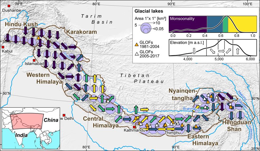
4146                  M. Fischer et al.: Controls of outbursts of moraine-dammed lakes in the greater Himalayan region

snow event early in the monsoon season (Allen et al., 2016).      the occurrence probability of GLOFs and thus reduce the in-
This particularly destructive GLOF underlines the need for        herent subjective bias (Emmer and Vilímek, 2013). For ex-
understanding better how and why meltwater lakes can be           ample, Wang et al. (2011) classified the outburst potential of
susceptible to sudden outburst triggered by rainstorms, es-       moraine-dammed lakes on the southeastern Tibetan Plateau
pecially given projected impacts of atmospheric warming on        by applying a fuzzy consistent matrix method. They used as
the high-mountain cryosphere.                                     inputs the size of the parent glacier, the distance and slope be-
   Current scenarios entail that atmospheric warming may          tween lake and glacier snout, and the mean steepness of the
change the susceptibility of HKKHN glacial lakes to sud-          moraine dam and the glacier snout to come up with different
den outburst floods: the IPCC’s (Intergovernmental Panel          nominal hazard categories. This and many similar qualitative
on Climate Change) most recent projections attribute the          ranking schemes are accessible to a broader audience and
decay of low-lying glaciers and permafrost to increases in        policy makers but are difficult to compare, and they poten-
lake number and area because of rising air temperatures,          tially oversimplify uncertainties.
more frequent rain-on-snow events at higher elevations, and           One way to deal with these uncertainties in a more ob-
changes in precipitation seasonality (Hock et al., 2019). Air     jective way involves a Bayesian approach. Here we used this
surface temperature in the HKKHN rose by about 0.1 ◦ C per        probabilistic reasoning with data-driven models. Specifically,
decade from 1901 to 2014 (Krishnan et al., 2019), likely          we tested how well some of the more widely adopted predic-
having reduced snowfall, altered permafrost distribution, and     tors of GLOF susceptibility and hazard fare in a multi-level
accelerated glacier melt at lower elevations (Hock et al.,        logistic regression that is informed more by data rather than
2019). Ice loss in the Himalayas has significantly increased      by expert opinion. We checked how well this approach iden-
in the past four decades, from −0.22 ± 0.13 m w.e. yr−1 (me-      tifies glacial lakes in the HKKHN that had released GLOFs in
tres of water equivalent per year) between 1975 and 2000          the past four decades. Our method estimates the probability
to −0.43 ± 0.14 m w.e. yr−1 between 2000 and 2016 (Mau-           of correctly detecting historic GLOFs from a set of predictors
rer et al., 2019). Parts of this meltwater have been trapped      which act as proxies subsuming various physical processes
in glacial lakes that have expanded by approximately 14 %         described as being relevant to GLOFs. Triggering mecha-
between 1990 and 2015 (Nie et al., 2017). King et al.             nisms of these GLOFs are rarely reported, however. Thus,
(2019) found that Himalayan glaciers terminating in lakes         we discuss what more we can learn about how these historic
had higher rates of mass loss since the 1970s than those not      GLOFs were linked to readily available measures of topogra-
in direct contact with a glacial lake. The notion of elevation-   phy, monsoonality, and glaciological changes. Our model re-
dependent warming (EDW) posits that increases in air tem-         sults provide a posterior probability of outburst conditioned
perature are most pronounced at higher elevations (Hock           on detection, and this may be used as a relative metric of
et al., 2019; Pepin et al., 2015). EDW has affected cold tem-     GLOF release from a given lake. Therefore, our approach is
perature metrics, including the number of frost days and min-     an alternative to a formal assessment of moraine-dam stabil-
ima of near-surface air temperature in the HKKHN in the           ity, which is (geo-)technically feasible only at selected sites
past decades (Krishnan et al., 2019; Palazzi et al., 2017). Es-   and at scales much finer than our regional and decadal focus.
sentially, all scenarios of atmospheric warming concern as-
pects of elevation, glacial lake size and dynamics, and local
climatic variability. Yet whether and how these aspects affect    2     Study area, data, and methods
GLOF hazards still awaits more quantitative support.
   Previous work on GLOF susceptibility and hazard in the         2.1    Study area and data
region focused on identifying or classifying potentially un-
stable glacial lakes, including local case studies largely in-    We studied glacial lakes of the Hindu Kush–Karakoram–
formed by fieldwork, dam-breach models (Koike and Take-           Himalayas–Nyainqentanglha (HKKHN) region that we de-
naka, 2012; Somos-Valenzuela et al., 2012, 2014), and basin-      fined here as the Asian mountain ranges between 16 to
wide assessments (Bolch et al., 2011; Mool et al., 2011;          39◦ N and 61 to 105◦ E, i.e. from Afghanistan to Myan-
Rounce et al., 2016; Wang et al., 2011). GLOF hazard ap-          mar (Fig. 1; Bajracharya and Shrestha, 2011). Following the
praisals for the entire HKKHN, however, remain rare (Veh          outlines of glacier regions in High Mountain Asia used in
et al., 2020). Most basin-wide studies proposed qualitative       the Randolph Glacier Inventory version 6.0 (RGI Consor-
to semi-quantitative decision schemes using selective lists of    tium, 2017) and those defined by Brun et al. (2017), Veh
presumed GLOF predictors (Table 1; Rounce et al., 2016).          et al. (2020) subdivided our study area into seven moun-
Yet researchers have used subjective rules to choose these        tain ranges: the Hindu Kush, the Karakoram, the Western
variables and associated thresholds, leading to diverging haz-    Himalaya, the Central Himalaya, the Eastern Himalaya, the
ard estimates (Rounce et al., 2016). Expert knowledge has         Nyainqentanglha, and the Hengduan Shan. Meltwater from
thus been essential in GLOF hazard appraisals despite an          the HKKHN’s extensive snow and ice cover, often referred
increasing amount of freely available climatic, topographic,      to as the “Third Pole”, feeds 10 major river systems to
and glaciological data. Statistical models can help to estimate   provide water for some 1.3 billion people (Molden et al.,

The Cryosphere, 15, 4145–4163, 2021                                                   https://doi.org/10.5194/tc-15-4145-2021

M. Fischer et al.: Controls of outbursts of moraine-dammed lakes in the greater Himalayan region                                                           4147

Table 1. Frequently used predictors of GLOF susceptibility and hazard in the HKKHN.

   Predictor         GLOF susceptibility and            Tested in    Reference
   groups            hazard predictors                  this study
   Lake              Glacial lake elevation             X            Mergili and Schneider (2011)
   characteristics
                     Catchment area                     X            Allen et al. (2019); GAPHAZ (2017)
   and dynamics
                     Glacial lake area                  X            Aggarwal et al. (2016); Allen et al. (2019); Bolch et al. (2011); GAPHAZ (2017); Ives
                                                                     et al. (2010); Khadka et al. (2021); Mergili and Schneider (2011); Prakash and Nagara-
                                                                     jan (2017); Wang et al. (2012); Worni et al. (2013)
                     Lake-area change (growth and       X            Aggarwal et al. (2016); Bolch et al. (2011); Ives et al. (2010); Khadka et al. (2021);
                     shrinkage, absolute change)                     Mergili and Schneider (2011); Prakash and Nagarajan (2017); Rounce et al. (2016);
                                                                     Wang et al. (2012)
   Potential         Lake volume                        –            Aggarwal et al. (2016); Bolch et al. (2011); GAPHAZ (2017); Kougkoulos et al. (2018);
   downstream                                                        Mergili and Schneider (2011)
   impact
   Dam stability     Moraine-wall steepness             –            Allen et al. (2019); Bolch et al. (2011); Dubey and Goyal (2020); GAPHAZ (2017);
                                                                     Ives et al. (2010); Khadka et al. (2021); Prakash and Nagarajan (2017); Rounce et al.
                                                                     (2016); Wang et al. (2011); Worni et al. (2013)
                     Width-to-height ratio              –            Aggarwal et al. (2016); Bolch et al. (2011); GAPHAZ (2017); Ives et al. (2010); Prakash
                                                                     and Nagarajan (2017); Worni et al. (2013)
                     Lake freeboard                     –            Bolch et al. (2011); GAPHAZ (2017); Kougkoulos et al. (2018); Mergili and Schneider
                                                                     (2011); Prakash and Nagarajan (2017); Worni et al. (2013)
                     Existence of a buried ice core     –            Bolch et al. (2011); Dubey and Goyal (2020); GAPHAZ (2017); Ives et al. (2010);
                                                                     Rounce et al. (2016)
                     Dam type                           X            GAPHAZ (2017); Kougkoulos et al. (2018); Mergili and Schneider (2011); Wang et al.
                                                                     (2011); Worni et al. (2013)
                     Moraine lithology                  –            GAPHAZ (2017)
   Potential         Seismic activity                   –            GAPHAZ (2017); Ives et al. (2010); Kougkoulos et al. (2018); Mergili and Schneider
   triggering                                                        (2011); Prakash and Nagarajan (2017)
   mechanisms
                     Distance from parent glacier       –            Aggarwal et al. (2016); Ives et al. (2010); Khadka et al. (2021); Kougkoulos et al.
   (geomorphic)
                     snout                                           (2018); Prakash and Nagarajan (2017); Wang et al. (2011, 2012); Worni et al. (2013)
                     Steepness parent glacier snout     –            Bolch et al. (2011); Ives et al. (2010); Kougkoulos et al. (2018); Prakash and Nagarajan
                                                                     (2017); Wang et al. (2011)
                     Parent glacier calving potential   –            GAPHAZ (2017); Ives et al. (2010); Mergili and Schneider (2011)
                     (width, crevasse density)
                     Regional or parent glacier-mass    X            Bolch et al. (2011); Ives et al. (2010)
                     balance
                     Mass movements (traces, tra-       –            Allen et al. (2019); Bolch et al. (2011); Dubey and Goyal (2020); GAPHAZ (2017);
                     jectories, probabilities)                       Ives et al. (2010); Khadka et al. (2021); Mergili and Schneider (2011); Prakash and
                                                                     Nagarajan (2017); Rounce et al. (2016); Worni et al. (2013)
                     Permafrost conditions              –            GAPHAZ, 2017
                     Upstream lake (with GLOF po-       –            Dubey and Goyal (2020); GAPHAZ (2017); Khadka et al. (2021)
                     tential)
   Potential         Annual mean temperature            –            GAPHAZ (2017); Liu et al. (2014); Wang et al. (2008)
   triggering
                     Temperature seasonality            –            Ives et al. (2010); Kougkoulos et al. (2018)
   events
   (climatic)        Temperature extremes (inten-       –            GAPHAZ (2017)
                     sity, frequency)
                     Annual precipitation               –            Wang et al. (2008, 2012)
                     Precipitation seasonality          –            Ives et al. (2010); Kougkoulos et al. (2018)
                     Precipitation extremes (inten-     –            GAPHAZ (2017); Prakash and Nagarajan (2017)
                     sity, frequency)
                     Summer precipitation or proxy      X            Wang et al. (2008, 2012)
                     of monsoonality

https://doi.org/10.5194/tc-15-4145-2021                                                                        The Cryosphere, 15, 4145–4163, 2021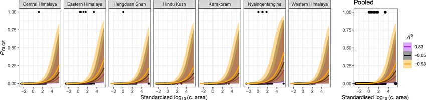
4148                    M. Fischer et al.: Controls of outbursts of moraine-dammed lakes in the greater Himalayan region

Figure 1. Overview map of the HKKHN showing the distribution of moraine-dammed lakes in 1◦ × 1◦ bins (blue bubbles scaled by area),
their elevation (expressed as quantiles coded by arrows; see inset for elevation distribution), and average monsoonality (colour coded; see
inset for monsoonality distribution), defined here as the fraction of total annual precipitation falling in the summer months. Orange and white
triangles indicate reported moraine-dam failures before and after 2005, respectively (Veh et al., 2019). Background hillshade is from the
GTOPO30 global 30 arcsec elevation dataset (https://doi.org/10.5066/F7DF6PQS).

2014). There, glaciers have had an overall negative mass                  bility of low-lying moraine dams may be compromised by
balance historically and lost 150 ± 110 kg m−2 yr−1 on av-                the loss of permafrost and commensurate increases in per-
erage from 2006 to 2015, though with balanced trends in                   meability in the moraine barrier and adjacent valley slopes
the Karakoram (Bolch et al., 2019; Hock et al., 2019). Since              (Haeberli et al., 2017).
the 1970s, some Karakoram glaciers also accelerated in flow,                 Glacial lake area A (m2 ) and its rate of change 1A (net
whereas glaciers stalled elsewhere in the HKKHN (Dehecq                   change) and A∗ (relative change, %) are other common pre-
et al., 2019). In the RCP8.5 scenario the HKKHN glaciers                  dictors of susceptibility and hazard in GLOF studies (Allen
could lose 64 ± 5 % of their total mass by 2100 compared                  et al., 2019; Bolch et al., 2011; Prakash and Nagarajan, 2017;
to estimated glacier volumes for the interval 1995 to 2015                see Table 1 for full list of references) that we considered
(Kraaijenbrink et al., 2017). How much of this melting of                 here. Due to a general lack of available bathymetric data
glaciers is due to EDW remains under debate (Palazzi et al.,              on a regional scale, a number of studies used the frequently
2017; Rangwala and Miller, 2012; Tudoroiu et al., 2016).                  observed phenomenon that lake area scales with lake vol-
Snowfall at lower elevations is also likely to decrease (Hock             ume and depth (Huggel et al., 2002; Iribarren Anacona et al.,
et al., 2019; Terzago et al., 2014), judging from snowfall and            2014). Growing lake depths increase the hydrostatic pressure
glacier-mass balances of past decades (Kapnick et al., 2014;              acting on moraine dams, thus raising the potential of fail-
King et al., 2019). Monsoon precipitation is likely to become             ure (Iribarren Anacona et al., 2014; Rounce et al., 2016). In
more episodic and intensive (Palazzi et al., 2013).                       the past decades, lake areas have grown largest in the Cen-
   Guided by these projections, we selected several widely                tral Himalayas (+23 % in 1990–2015; Nie et al., 2017) and
used glacial lake susceptibility predictors (Table 2).                    Nyainqentanglha Mountains but lowest in the northwestern
   We used lake elevation z (m a.s.l.) as a proxy for the                 Himalayas (Chen et al., 2021; Nie et al., 2017), and many
standard lapse rate of tropospheric air temperature (Rol-                 studies have emphasised the role of growing lakes on GLOF
land, 2003; Yang and Smith, 1985). This elevation-dependent               susceptibility (e.g. GAPHAZ, 2017; Prakash and Nagarajan,
thermal gradient is also a major control on the distribution              2017; Rounce et al., 2016). Many previous GLOF assessment
of alpine permafrost (Etzelmüller and Frauenfelder, 2009)                 schemes included lake area or lake-area growth as a proxy for
and precipitation. Mean annual rainfall along the Himalayan               the volume of water that could be potentially released by an
front can exceed 4000 mm at elevations some 4000 m high,                  outburst and thus the resulting downstream hazard (e.g. Allen
where ∼ 25 % of all glacial lakes occur (Fig. 1; Bookhagen                et al., 2019; Bolch et al., 2011). However, a number of studies
and Burbank, 2010). Lake elevation should also represent                  also stress that lake area and its growth define the exposure to
first-order topographic effects of EDW. For example, the sta-             external and internal triggers of moraine dam breach: larger

The Cryosphere, 15, 4145–4163, 2021                                                            https://doi.org/10.5194/tc-15-4145-2021
M. Fischer et al.: Controls of outbursts of moraine-dammed lakes in the greater Himalayan region                                                           4149

Table 2. Details on tested predictors and our reasoning for selection based on their commonly reported physical links to GLOF susceptibility.

   GLOF susceptibility      Symbol                          Unit          Data source          Selection reasoning
   predictor
   Glacial lake elevation   z                               m a.s.l.      SRTM DEM             – strong link between elevation and temperature at high al-
                                                                                               titudes (standard lapse rate of tropospheric air temperature)
                                                                                               → elevation dependence of permafrost and precipitation
                                                                                               patterns
   Catchment area           C                               m2            SRTM DEM             – potential for surface runoff into lake from precipitation
                                                                                               and snow melt
   Glacial lake area        A                               m2            SRTM DEM             – proxy for lake volume and depth and thus hydrostatic
                                                                                               pressure acting on moraine dam
   Lake-area change         1A       Net change             –             Wang et al. (2020)   – increasing lake area commonly reported as scaling with
                                                                                               increasing lake depth
                            A∗       Relative change        %
                                                                                               → potentially increased hydrostatic pressure acting on the
                                     (between)
                                                                                               moraine dam
                                     A∗a (1990–2005)                                           – increased proximity to steep valley slopes
                                     A∗b (2005–2018)                                           → increased potential of mass movements entering the lake
                                     A∗c (1990–2018)
   Glacier-mass balance     r        Glacier-mass balance   –             Brun et al. (2017)   – proxy for direct or surface runoff glacier meltwater input,
                                     region                                                    calving potential of parent glacier front, and permafrost dis-
                                                                                               tribution in lake surroundings
                            1mr      Average glacier-mass   m w.e. yr−1
                                                                                               – link between regional glacier-mass balance and synoptic
                                     balance
                                                                                               regime (winter westerlies vs. monsoon dominated)

   Monsoonality             M                               % (mm)        CHELSA               – high-intensity precipitation events during monsoon season
   (annual proportion of                                                  (Karger et al.,      potentially leading to increased surface runoff into glacial
   summer precipitation)                                                  2017)                lakes (cloudburst event)
                                                                                               – seasonal increases in lake levels and, hence, lake depths
                                                                                               increasing hydrostatic pressure acting on moraine dam
                                                                                               – link between regional glacier-mass balance and synoptic
                                                                                               regime (winter westerlies vs. monsoon dominated)

and growing lakes offer more area for impacts from mass                          1m (m water equivalent yr−1 ) from Brun et al. (2017). These
flows such as avalanches, rockfalls, and landslides originat-                    readily available data on regional glacier-mass balances are
ing from adjacent valley slopes (GAPHAZ, 2017; Haeberli                          proxies for other, less accessible physical controls on GLOF
et al., 2017; Prakash and Nagarajan, 2017; Rounce et al.,                        susceptibility such as glacial meltwater input, either directly
2016). Some authors also link growing lake areas to an in-                       from the parent glacier or from glaciers upstream, as well as
crease in hydrostatic pressure acting on its moraine dam, thus                   permafrost decay in slopes fringing the lake (see Table 2 for
making the latter more susceptible to sudden failure (Iribar-                    full list).
ren Anacona et al., 2014; Mergili and Schneider, 2011).                             Meteorological drivers entered previous qualitative GLOF
   We also tested the impact of upstream catchment area C                        hazard appraisals mostly as (the probability of) extreme mon-
(m2 ) on GLOF susceptibility. A larger upstream catchment                        soonal precipitation events: the Kedarnath GLOF disaster,
area has been associated with an increased susceptibility                        for example, was triggered by intense surface runoff (Huggel
to GLOFs as runoff from intense precipitation, as well as                        et al., 2004; Prakash and Nagarajan, 2017). Heavy rainfall
glacier and snow melt, can lead to sudden increases in lake                      may also trigger landslides or debris flows from adjacent hill-
volume (Allen et al., 2019; GAPHAZ, 2017). We find that                          slopes followed by displacement waves that overtop moraine
catchment area C correlates with lake area A (Pearson’s                          dams (Huggel et al., 2004; Prakash and Nagarajan, 2017).
ρ = 0.45). We thus preferred C over A in two of our mod-                         Elevated lake levels during the monsoon season also raise
els as C is invariant at the timescale of our study, and we use                  the hydrostatic pressure acting on moraine dams (Richard-
these two models to explicitly test whether runoff by glacier                    son and Reynolds, 2000). Furthermore, different precipita-
melt or monsoonal precipitation had an effect on GLOFs in                        tion regimes and climatic preconditions may also influence
our study area.                                                                  moraine-dam failure mechanics (Wang et al., 2012). Intense
   Similar to changes in lake area, glacier dynamics are fre-                    precipitation occurs in our study region largely during the
quently mentioned though rarely incorporated quantitatively                      summer monsoon, so we derived a synoptic measure of mon-
in susceptibility appraisals (Bolch et al., 2011; Ives et al.,                   soonality M (%). We define monsoonality M in terms of the
2010). This motivated us to consider the average changes                         annual proportion of summer, i.e. the warmest quarter, pre-
in regional glacier-mass balances between 2000 and 2016                          cipitation, which is highest in the southeast HKKHN, where

https://doi.org/10.5194/tc-15-4145-2021                                                                    The Cryosphere, 15, 4145–4163, 2021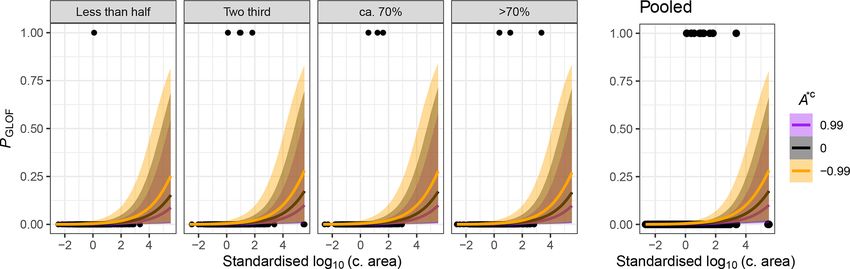
4150                    M. Fischer et al.: Controls of outbursts of moraine-dammed lakes in the greater Himalayan region

it is linked to monsoonal low-pressure systems (Krishnan          Here α0 is the intercept, and β = {β1 , . . ., βpT } are the p pre-
et al., 2019).                                                    dictor weights (Gelman and Hill, 2007). The logit function
   We extracted information on these characteristics for          S −1 (x) describes the odds on a logarithmic scale (the log-
glacial lakes recorded in two inventories. First, we used the     odds ratio) such that a unit increase in predictor xm raises the
ICIMOD database of 25 614 lakes manually mapped from              log-odds ratio by an amount of βm , with all other predictors
Landsat imagery acquired in 2005 ± 2 years (Maharjan et al.,      fixed. We used standardised data to ensure that the weights
2018), from which we extracted 7284 lakes dammed by               measure the relative contributions of their predictors to the
moraines (classes m(l), m(e), and m(o) in Maharjan et al.,        classification, whereas the intercept expresses the base case
2018). Second, we identified from an independent regional         for average predictor values.
GLOF inventory (Veh et al. 2019) 31 lakes that had at least          Our strategy was to explore commonly reported predic-
one outburst between 1981 and 2017 and that are listed in         tors of GLOF susceptibility and dam stability as candidate
the ICIMOD inventory. The triggering mechanism of these           predictors (Fig. 2, Tables 1 and 2). We further acknowledged
studied GLOFs is reported in only seven cases, four of which      that data on moraine-dammed lakes in the HKKHN are struc-
are attributed to ice avalanches entering the lake (e.g. Tam      tured, reflecting, for example, the variance in topography and
Pokhari, Nepal, and Kongyangmi La Tsho, India; Ives et al.,       synoptic regime such as the summer monsoon in the east-
2010; Nie et al., 2018). Other triggers of the GLOFs studied      ern HKKHN and westerlies in the western HKKHN. Dif-
here include piping (Yindapu Co, China; Nie et al., 2018) and     ferent data sources, collection methods, and resolutions also
the collapse of an ice-cored moraine (Luggye Tsho, Bhutan;        add structure. This structure is routinely acknowledged, often
Fujita et al., 2008). We focused on lakes > 10 000 m2 to en-      raised as a caveat, but rarely treated in GLOF studies. Ignor-
sure comparability between the two inventories, thus acquir-      ing such structure can lead to incorrect inference by bloat-
ing a final sample size of 3390 lakes. Given the sparse net-      ing the statistical significance of irrelevant or inappropriate
work of weather stations in the HKKHN, we computed the            model parameter estimates (Austin et al., 2003). To explicitly
monsoonality averaged for each lake from the 1 km resolu-         address this issue, we chose a multi-level logistic regression
tion CHELSA bioclimatic variables (Karger et al., 2017).          as a compromise between a single pooled model and individ-
These variables are correlated with elevation because of the      ual models for each group in the data (Fig. 3; Gelman and
same underlying interpolation technique, so we limited our        Hill, 2007; Shor et al., 2007).
models to those with poorly correlated predictors. This meant        We recast Eq. (2) using a group index j :
omitting other predictors such as mean annual temperature,
annual precipitation totals, and annual temperature and pre-      µi = S(αj + β1 xi,1 + β2 xi,2 + . . . + βp xi,p ),             (4)
cipitation variability. We extracted topographic data from        αj ∼ N (µα σα ),                                               (5)
the void-free 30 m resolution SRTM (Shuttle Radar Topo-
graphic Mission of 2000) digital elevation model (DEM) and        where µα is the mean, and σα is the standard deviation of
use approximate lake-area changes for two intervals (1990         the group-level intercepts αj that are learned from all data
to 2005 and 2005 to 2018) by Wang et al. (2020). We dis-          and inform each other via the model hierarchy. We used a
carded newer, higher-resolved DEMs to minimise data gaps          Bayesian framework (Kruschke and Liddell, 2018) by com-
and artefacts. Overall, we considered six topographic, synop-     bining the likelihood of observing the data with prior knowl-
tic, and glaciological predictors (Fig. 2, Table 2).              edge from previous GLOF studies (Fischer et al., 2020). The
                                                                  small number of reported GLOFs introduces strong imbal-
2.2    Bayesian multi-level logistic regression                   ance to our data given that some regions, and hence lev-
                                                                  els, had few or no reported GLOFs. Although this would be
We used logistic regression to learn the probability of           problematic in most other modelling approaches, Bayesian
whether a given lake in the HKKHN had a reported                  multi-level models are well suited for this kind of imbal-
GLOF in the past four decades. This method was pioneered          anced training data (Gelman and Hill, 2007; Shor et al., 2007;
for moraine-dammed lakes in British Columbia, Canada              Stegmueller, 2013).
(McKillop and Clague, 2007). Logistic regression estimates           We used the statistical programming language R with the
a binary outcome y from the optimal linear combination            package brms, which estimates joint posterior distributions
of p weighted predictors x = {x1 , . . ., xp }. The probability   using a Hamiltonian Monte Carlo algorithm and a No-U-
y = PGLOF that lake i had released a GLOF is expressed as         Turn Sampler (NUTS; Bürkner, 2017). We ran four chains
follows:                                                          of 1500 samples after 500 warm-up runs each and checked
yi ∼ Bernoulli(µi ),                                       (1)    for numerical divergences or other pathological issues. We
µi = S(α0 + β1 xi,1 + β2 xi,2 + . . . + βp xi,p ),         (2)    only considered models with all values of R̂ < 1.01 – a mea-
                                                                  sure of numerical convergence of sampling chains – to avoid
where                                                             unbiased posterior distributions (Nalborczyk et al., 2019).
               1                                                     Unless stated otherwise, we used a weakly informative
S(x) =               .                                     (3)    half Student’s t distribution with three degrees of freedom
         1 + exp(−x)

The Cryosphere, 15, 4145–4163, 2021                                                    https://doi.org/10.5194/tc-15-4145-2021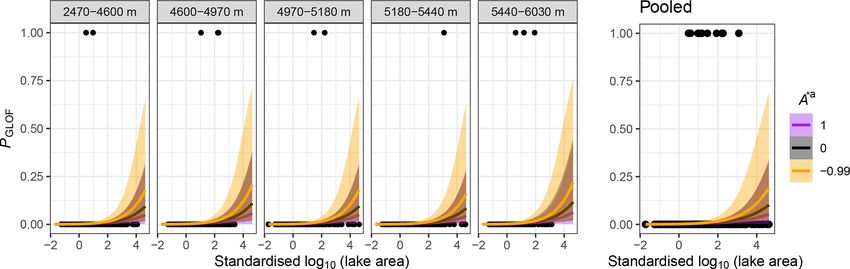
M. Fischer et al.: Controls of outbursts of moraine-dammed lakes in the greater Himalayan region                              4151

Figure 2. Data sources and workflow; EDW = elevation-dependent warming.

Table 3. Prior distributions for group- and population-level effects.

                 Level                      Model coefficient                                Probability density function
                 Group-level effects        Standard deviation σ of group model variables    σα ∼ HalfStudentT(3, 10)
                 Population-level effects   Intercept                                        αj ∼ Cauchy(0, 2.5)
                                            Weight of predictors with weak prior knowledge   βp ∼ Cauchy(0, 2.5)
                                            Weight of predictor lake area βA                 βA ∼ Normal(1, 2)

                                                                        and a scale parameter of 10 for the standard deviations of
                                                                        group-level effects (Table 3; Bürkner, 2017; Gelman, 2006).
                                                                        At the population level, we chose weakly informative pri-
                                                                        ors for the intercept and coefficients for which we had no
                                                                        other prior knowledge. We encoded this lack of knowledge
                                                                        with a prior Cauchy distribution centred at zero and with
                                                                        a scale of 2.5, following the recommendation of Gelman
Figure 3. Schematic comparison of global vs. multi-level logistic
regression models.
                                                                        et al. (2008). Rapidly growing moraine-dammed lakes are
                                                                        a widely used predictor of high GLOF susceptibility (e.g.
                                                                        GAPHAZ, 2017; Prakash and Nagarajan, 2017; Rounce et

https://doi.org/10.5194/tc-15-4145-2021                                                      The Cryosphere, 15, 4145–4163, 2021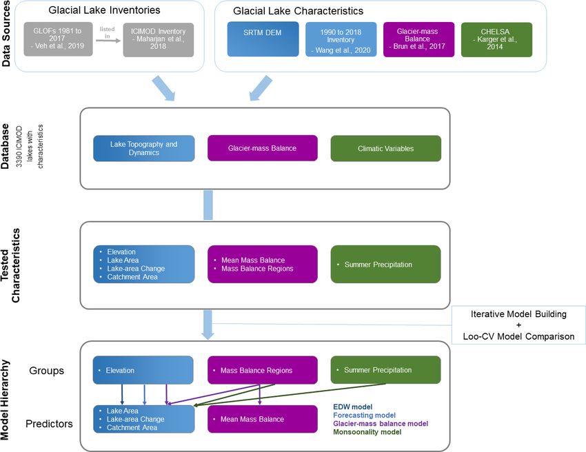
4152 M. Fischer et al.: Controls of outbursts of moraine-dammed lakes in the greater Himalayan region
al., 2016). We encoded this notion in a prior Gaussian dis- 3.2 Forecasting model
tribution with 1 unit mean and standard deviation, hence
shifting more probability mass towards positive regression Our second model refines our approach by including only
weights without excluding the possibility of negative weight relative changes in lake area before the reported GLOFs hap-
estimates (Table 3). pened. We can use this model to fore- or hindcast historic
We estimated the predictive performance of all models GLOFs in our inventory. Here we use lake area A (in 2005)
with leave-one-out (LOO) cross-validation as part of the and its relative change A∗a from 1990 to 2005 as predictors
brms package (Bürkner, 2017). LOO values like the expected of 11 GLOFs that occurred between 2005 and 2018 across
log predictive density (ELPD) summarise the predictive error the five elevation bands. We assume that larger and deeper
of Bayesian models similar to the Akaike information cri- lakes are more robust to relative size changes and thus also
terion or related metrics of model selection (Vehtari et al., include a multiplicative interaction term between lake area
2017). They are based on the log-likelihood of the posterior and its change:
simulations of parameter values (Vehtari et al., 2017).
µi = S αz + βA Ai + βA∗a A∗a ∗a
i + βA×A∗a Ai · Ai . (8)
3 Results
We find that lake area has a credible positive posterior
3.1 Elevation-dependent warming model weight of βA = 0.86+0.44 /−0.43 ; hence greater lakes are more
likely to have had a GLOF between 2005 and 2018. The
Our first model addresses the notion of elevation-dependent weight of relative lake-area change in the 15 years before is
warming (EDW) by considering lake elevation as a group- ambiguous (βA∗a = −0.04+0.76 /−0.67 ) and so is the interac-
ing structure in the data. The model further assumes that the tion (βA·A∗a = −0.16+0.41 /−0.51 ). On average, however, rel-
GLOF history of a given lake is a function of its area A and ative increases in lake area between 1990 and 2005 slightly
net change 1A. This dependence differs by up to a constant, decrease PGLOF . Unlike in the elevation-dependent warming
i.e. the varying model intercept, across elevation bands z model, the effects of elevation bands are less clear, while the
that we define here in five quantile grouping levels (Fig. 1). uncertainties are more pronounced and highest for larger and
The model intercept may vary across these elevation bands, shrinking lakes (Figs. 4 and 6).
whereas lake area (in 2005) and its net change remain fixed
predictors. In essence, this varying-intercept model acknowl- 3.3 Glacier-mass balance model
edges that glacial lakes in the same elevation band may have
had a common baseline susceptibility to GLOFs in the past Besides elevation, our third model considers the average his-
four decades. The indicator variable 1A records whether a toric glacier-mass balances across the HKKHN. The model
given lake had a net growth or shrinkage between 1990 and assumes that mean ice losses 1m add a distinctly regional
2018: structure to the susceptibility to GLOFs in the past four
decades given that accelerated glacier melt may raise GLOF
µi = S(αz + βA Ai + β1A 1Ai ), (6) potential (Emmer, 2017; Richardson and Reynolds, 2000).
We use our seven study area regions as group levels r and
αz ∼ N (µz σz ), (7)
their average glacier-mass balance, derived from Brun et al.
where index z identifies the elevation band. (2017), as a group-level predictor 1mr . Our pooled predic-
We obtain posterior estimates of βA = 0.79+0.27 /−0.27 and tors are the relative change in lake area A∗b from 2005 to
β1A = 0.48+0.73 /−0.72 (95 % highest density interval, HDI) 2018 (to ensure a comparable time interval) and the catch-
which indicate that larger lakes are more likely classified as ment area C upstream of each lake. We replace lake area by
having had a GLOF, whereas net growth or shrinkage has its upstream catchment area, which is less prone to change
ambivalent weight as its HDI includes zero (Figs. 4 and 5, Ta- but well correlated to lake area.
ble 4). On the population level, the low spread of intercepts
µi = S αz + αr + βA∗b A∗b i + βC C i , (9)
(σz = 0.29+0.68 /−0.28 ) estimated for each of the five eleva-
tion bands shows that elevation effects modulate the pooled αr ∼ N (µr + γr 1mr σr ). (10)
model only minutely. These posterior effects are positive for
the lower elevation bands but negative for the higher eleva-
tion bands. Thus, the mean posterior probability of a GLOF This model returns a positive weight for catchment area
history, PGLOF , under this model increases slightly for lakes (βC = 0.85+0.50 /−0.50 ) and a negative weight for relative
in lower elevations and with a larger surface area in 2005. lake-area changes (βA∗b = −0.69+0.64 /−0.61 ), whereas the
We also observe that PGLOF is less than 0.5 regardless of re- effect of the mean glacier-mass balance remains inconclu-
ported lake elevation and that the associated uncertainties are sive (γr = −2.98+4.87 /−6.70 ). On the basis of higher standard
higher for larger lakes. deviations, we learn that effects of glaciological regions vary
more than those of elevation bands (σr = 0.81+1.60 /−0.78 and
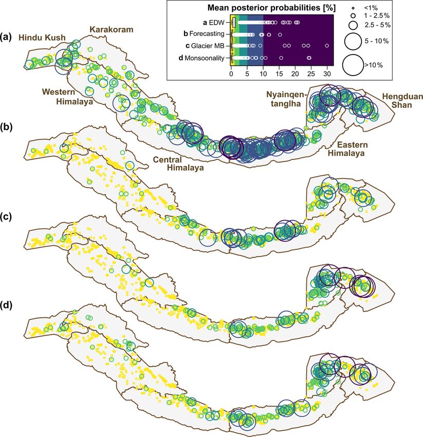
The Cryosphere, 15, 4145–4163, 2021 https://doi.org/10.5194/tc-15-4145-2021M. Fischer et al.: Controls of outbursts of moraine-dammed lakes in the greater Himalayan region 4153
Figure 4. Posterior pooled and group-level intercepts for the four models considered. EDW = elevation-dependent warming. See Fig. 1 for a
summary of the quantiles of elevation and monsoonality. Horizontal black lines delimit 95 % HDI, and red circles indicate posterior medians.
Vertical continuous (dashed) grey lines are posterior means (95 % HDI) of the pooled intercept of each model. Intercepts are standardised
and thus refer to lakes with average predictor values.
σz = 0.48+1.19 /−0.47 ). When training this model on a sub- 3.4 Monsoonality model
set of glacial lakes with documented GLOFs that happened
after 2000 (i.e. including only those in the interval covered Our last model explores a synoptic influence on GLOF sus-
by glacier-mass balance data), posterior estimates of σr in- ceptibility by grouping the data by the summer proportion
crease to 1.11+1.77 /−1.03 , further underlining our result that of mean annual precipitation and thus by approximate mon-
glacier-mass balance credibly affects PGLOF . This is also re- soonal contribution. We defined five monsoonality levels
flected in the posterior distributions across the glacier-mass based on quantiles of the annual proportions of summer pre-
balance regions (Fig. 4), as well as the calculated group-level cipitation (Fig. 1). We use relative lake-area change A∗c be-
effects. This model has the highest values of PGLOF for av- tween 1990 and 2018 and catchment area C as population-
erage lakes (i.e. all average predictor values combined) in level predictors, as well as the additional grouping by re-
the Nyainqentanglha Mountains and the Eastern Himalaya gional glacier-mass balance:
(Fig. 4). In contrast to the forecasting model, we observe that
increases in lake area now credibly depress PGLOF (Fig. 7).
µi = S αM + αr + βA∗c A∗c
i + βC Ci , (11)
αM ∼ N (µM σM ), (12)
https://doi.org/10.5194/tc-15-4145-2021 The Cryosphere, 15, 4145–4163, 20214154 M. Fischer et al.: Controls of outbursts of moraine-dammed lakes in the greater Himalayan region
Figure 5. Elevation-dependent warming model: posterior probabilities PGLOF as a function of standardised lake area A (in 2005) and
the sign of standardised lake-area change 1A (i.e. net growth or shrinkage), grouped by quantiles of elevation (defined in Fig. 1; lowest:
2470–4600 m a.s.l.; low: 4600–4970 m a.s.l.; medium: 4970–5180 m a.s.l.; high: 5180–5440 m a.s.l.; highest: 5440–6030 m a.s.l.). Black dots
are lake data with (PGLOF = 1) or without (PGLOF = 0) reported GLOF records. Thick coloured lines are mean fits, and colour shades
encompass the associated 95 % HDIs.
Table 4. Summary of the results of our four models. CI = credible interval.
Model Model parameter Estimate Estimation Lower 95 % CI Upper 95 % CI
error boundary boundary
Elevation-dependent αz −5.22 0.36 −5.96 −4.56
warming model βA 0.79 0.14 0.52 1.06
β1A (1990 to 2018) 0.49 0.38 −0.28 1.24
σz 0.28 0.27 0.01 0.99
Forecasting model αz −6.23 0.54 −7.39 −5.26
βA 0.87 0.22 0.44 1.31
βA∗a (1990 to 2005) −0.04 0.38 −0.71 0.73
βA·A∗a −0.16 0.24 −0.67 0.26
σz 0.43 0.41 0.01 1.49
Glacier-mass αz,r −7.31 1.26 −10.15 −5.19
balance model βA∗b (2005 to 2018) −0.69 0.32 −1.31 −0.06
βC 0.85 0.26 0.35 1.36
γr −2.90 2.80 −9.27 1.80
σz 0.47 0.44 0.01 1.61
σr 0.83 0.66 0.03 2.47
Monsoonality αM,r −6.14 0.70 −7.70 −4.91
model βA∗c (1990 to 2018) −0.63 0.31 −1.23 −0.02
βC 0.82 0.24 0.34 1.28
σM 0.40 0.42 0.01 1.49
σr 0.78 0.62 0.03 2.31
where index M identifies the monsoonality group. We find 3.5 Model performance and validation
that larger catchment areas (βC = 0.82+0.46 /−0.48 ) and lakes
with relative shrinkage (βA∗c = −0.63+0.59 /−0.59 ) credibly We estimate the performance of our models in terms of the
raise PGLOF (Figs. 4 and 8). Higher standard deviations posterior improvement of our prior chance of finding a lake
show that regional effects vary more for the mean glacial- with known outburst in the past four decades in our inven-
mass balance than for monsoonality (σr = 0.79+1.59 /−0.76 tory by pure chance. We compare the posterior predictive
and σM = 0.40+1.04 /−0.39 ), although both hardly change the mean PGLOF with a mean prior probability that we estimate
pooled model trend. from the ∼ 1 % proportion of lakes with known GLOFs in
our training data. We measure what we have learned from
each model in terms of the log-odds ratio that readily trans-
The Cryosphere, 15, 4145–4163, 2021 https://doi.org/10.5194/tc-15-4145-2021M. Fischer et al.: Controls of outbursts of moraine-dammed lakes in the greater Himalayan region 4155
Figure 6. Forecasting model: posterior probabilities PGLOF as a function of standardised lake area A (in 2005) and standardised lake-area
change A∗a between 1990 and 2005, grouped by quantiles of elevation (defined in Fig. 1; lowest: 2470–4600 m a.s.l.; low: 4600–4970 m a.s.l.;
medium: 4970–5180 m a.s.l.; high: 5180–5440 m a.s.l.; highest: 5440–6030 m a.s.l.). Black dots are lake data with (PGLOF = 1) or without
(PGLOF = 0) reported GLOF records for the interval 2005 to 2018. Thick coloured lines are mean fits, and colour shades encompass the
associated 95 % HDIs.
Figure 7. Glacier-mass balance model: posterior probabilities PGLOF as a function of standardised catchment area C and standardised lake-
area change A∗b between 2005 and 2018, grouped by regions of average glacier-mass balance (see Fig. 1). Black dots are lake data with
(PGLOF = 1) or without (PGLOF = 0) reported GLOF records for the interval 2005 to 2018. Thick coloured lines are mean fits, and colour
shades encompass the associated 95 % HDIs.
lates into probabilities using Eq. (3). A positive log-odds ra- 4 Discussion
tio means that we obtain a higher posterior probability of at-
tributing a historic GLOF to a given lake compared to a ran- 4.1 Topographic and climatic predictors of GLOFs
dom draw. Negative log-odd ratios indicate lakes for which
the posterior probability of a reported GLOF is lower than We used Bayesian multi-level logistic regression to test
the prior probability. Based on this metric, all models have whether several widely advocated predictors of GLOF sus-
higher true positive rates than true negative rates. For a prior ceptibility and glacial lake stability are credible predictors
probability informed by the historic frequency of GLOFs, the of at least one outburst in the past four decades. All four
models have at least about 80 % true positives and at least models that we considered identify lake area and catchment
70 % true negatives on average (Fig. 9, Table 5). area as predictors with weights that credibly differ from zero
The values of the LOO cross-validation of the predictive with 95 % probability. Our model results quantitatively sup-
capabilities show that the EDW model formally has the least port qualitative notions of several basin-wide studies in the
favourable, i.e. higher, values for both LOO metrics (Ta- HKKHN (e.g. Ives et al., 2010; Khadka et al., 2021; Prakash
ble 5). This is potentially due to the different true positive and Nagarajan, 2017) and elsewhere (McKillop and Clague,
counts in the training datasets. However, the range of esti- 2007), which proposed that larger moraine-dammed lakes
mated ELPD values between the remaining three models is have a higher potential for releasing GLOFs.
small (1ELPD = 1.9). We also found that changes in lake area have partly in-
conclusive influences in the models. Two exceptions are the
negative weight of lake-area changes βA∗b and βA∗c in the
glacier-mass balance model and in the monsoonality model
regardless of the differing intervals that these changes were
determined for (Table 4). While this result formally indicates
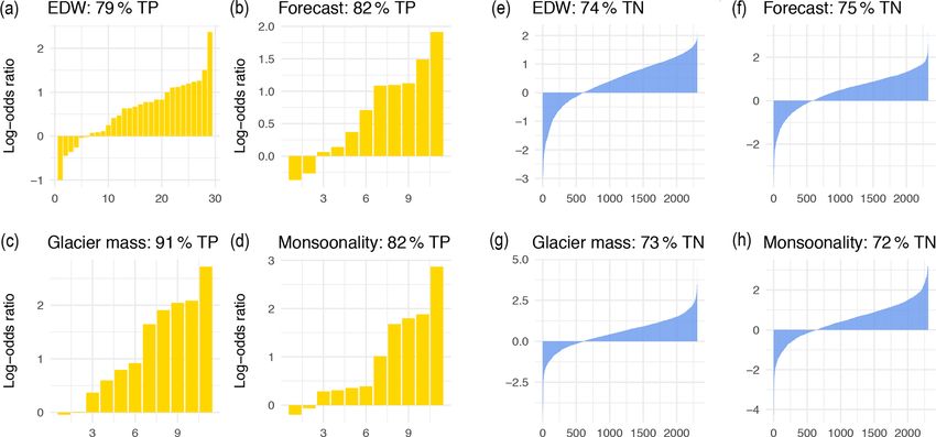
https://doi.org/10.5194/tc-15-4145-2021 The Cryosphere, 15, 4145–4163, 20214156 M. Fischer et al.: Controls of outbursts of moraine-dammed lakes in the greater Himalayan region Figure 8. Monsoonality model: posterior probabilities PGLOF as a function of standardised catchment area C and standardised lake-area change A∗c between 1990 and 2018, grouped by quantiles of the annual proportion of precipitation falling during summer (defined in Fig. 1). Black dots are lake data with (PGLOF = 1) or without (PGLOF = 0) reported GLOF records for the interval 1990 to 2018. Thick coloured lines are mean fits, and colour shades encompass the associated 95 % HDIs. Figure 9. Average posterior log-odds ratios for true positives (TP) (true negatives, TN), i.e. lakes with (without) a GLOF in the period 1981–2018 (a and e) and 2005–2018 (b–d and f–h) on the x axis for the four different models. The log-odds ratios describe here the ratio of the mean posterior over the mean prior probability of classifying a given lake as having had a GLOF. We estimate the mean prior probability from the relative frequency of GLOFs in the datasets. EDW = elevation-dependent warming model. that shrinking lakes are more likely to be classified as hav- warming model (Eq. 6). However, in the forecasting model, ing had a historic GLOF, the period over which these lake- in which we tested whether differing data observation pe- area changes are valid (2005 to 2018) overlaps with the tim- riods have any credible effects, the influence of lake-area ing of 11 recorded GLOFs (Eq. 9). In other words, the lake change remains negligible even for < 50 % HDIs. We thus shrinkage could be a direct consequence of these GLOFs conclude that relative lake-area change before outburst is an instead of vice versa. Nonetheless, our results indicate that inconclusive predictor. This result contradicts the assump- lake-area changes, either absolute or directional, are some- tions made in many previous studies that argued that rapidly what inconclusive in informing us whether a given lake has growing lakes are the most prone to sudden outburst (GAP- a recent GLOF history. One advantage of our Bayesian ap- HAZ, 2017; Iribarren Anacona et al., 2014; Ives et al., 2010; proach is that we can express the role of lake-area changes Mergili and Schneider, 2011; Prakash and Nagarajan, 2017; in GLOF susceptibility by choosing different highest den- Rounce et al., 2016). sity intervals. For example, if we adopted a narrower, say The role of elevation in GLOF predictions is also less pro- 80 % HDI for 1A, we could be 80 % certain that net lake- nounced than that of lake or catchment area, at least at a area growth increased PGLOF under the elevation-dependent group level. The weights of the elevation-dependent warm- The Cryosphere, 15, 4145–4163, 2021 https://doi.org/10.5194/tc-15-4145-2021
M. Fischer et al.: Controls of outbursts of moraine-dammed lakes in the greater Himalayan region                                 4157

Table 5. Overview of model validation measures for the predictive capabilities of our models. LOOIC = leave-one-out cross-validation
information criterion.

         Model                                          Prior vs. posterior knowledge             LOO cross-validation metrics
                                                % true positives/        % false positives/        ELPD               LOOIC
                                                % true negatives         % false negatives
                                                correctly identified     incorrectly identified
         Elevation-dependent warming model      79 %/74 %                21 %/26 %                −144.2                288.3
         Forecasting model                      82 %/75 %                18 %/25 %                 −66.5                132.9
         Glacier-mass balance model             91 %/73 %                9 %/27 %                  −64.6                129.1
         Monsoonality model                     82 %/72 %                18 %/28 %                 −65.6                131.2

ing model indicate that lower (higher) lakes are slightly              intercepts for comparable mean PGLOF and associated uncer-
more (less) likely to have had a historic GLOF (Fig. 4) but            tainties (Figs. 4, 7 and 8).
hardly warrant any better model performance compared to                   Our results offer insights into the links between historic
the pooled (or elevation-independent) model. In the forecast-          GLOFs and the synoptic precipitation patterns. Richard-
ing model, however, the contributions of lake elevation to             son and Reynolds (2000) presumed that seasonal floods and
PGLOF are devoid of any systematic pattern and likely reflect          GLOFs are both caused by high monsoonal precipitation and
several, potentially combined drivers (Fig. 4). This model             summer ablation. In contrast, our results indicate that the
was trained on fewer GLOFs, and the imbalance in the data              fraction of summer precipitation changes the predictive prob-
introduces more uncertainties in terms of broad 95 % HDIs.             abilities of historic GLOFs only marginally, at least at the
Clearly, the role of elevation may need more future inves-             group level, so that deviations from a pooled model for the
tigation. In terms of elevation bands, it hardly seems to aid          HKKHN are minute when compared to the spread of pos-
GLOF detection with the models used here. Similarly, Em-               terior group-level intercepts in the other models (Fig. 4). In
mer et al. (2016) reported that lake elevation was hardly af-          essence, our results underline the need for exploring more
fecting GLOF hazard in the Cordillera Blanca, Peru.                    the interactions of both precipitation and temperature as po-
   Judging from the regionally averaged glacier-mass bal-              tential GLOF triggers. It may well be that seasonal tim-
ances, our models predict the highest GLOF probabili-                  ing of heavy precipitation events and type (rain or snow)
ties in the Nyainqentanglha Mountains and the Eastern Hi-              at a given lake may be more meaningful to GLOF suscep-
malaya, which have had the highest historic GLOF counts                tibility than annual totals or averages. Whether our finding
(Fig. 1). The timing and seasonality of snowfall affect how            that glacier-mass balances driven by superimposed synop-
glaciers respond to rising air temperatures. Observed fre-             tic regimes credibly influence regional GLOF susceptibility
quencies and predicted probabilities of historic GLOFs are             in the HKKHN is applicable to other regions, for example
lowest for several glaciers with positive mass balance in the          the Cordillera Blanca in the South American Andes (Emmer
Karakoram and Western Himalaya (Figs. 1 and 10). Most                  et al., 2016; Emmer and Vilímek, 2014; Iturrizaga, 2011),
moraine-dammed lakes in the HKKHN, however, are fed by                 also needs further investigation.
glaciers with negative mass balances that likely help to ele-
vate GLOF potential through increased meltwater input and              4.2   Model assessment
glacier-tongue calving rates (Emmer, 2017; Richardson and
Reynolds, 2000). This is also supported by the findings of             We consider our quantitative and data-driven approach as
King et al. (2019), which imply that higher rates of mass loss         complementary to existing qualitative and basin-wide GLOF
of lake-terminating glaciers since the 1970s might have also           hazard appraisals. Our models cannot replace field observa-
led to increased meltwater input into lakes adjacent to their          tions that deliver local details on GLOF-disposing factors
termini. More than 70 % of all lakes that burst out in the past        such as moraine or adjacent rock-slope stability, presence of
four decades were in contact with their parent glaciers (Veh           ice cores, glacier calving rates, or surges. Our selection of
et al., 2019). However, systematically recorded time series            predictors is a compromise between widely used predictors
of glacier fronts are even harder to come by when compared             of GLOF susceptibility and hazard and their availability as
to systematic measurements of changes in glacial-lake areas.           data covering the entire HKKHN. To this end, we used lake
Given that the regional glacier-mass balance is linked to syn-         (or catchment) area and lake-area changes as predictors, as
optic precipitation patterns (Kapnick et al., 2014; King et al.,       well as elevation, regional glacier-mass balance, and mon-
2019; Krishnan et al., 2019), our glacier-mass balance model           soonality as group levels of past GLOF activity of several
highlights that the regional ice loss outweighs the role of            thousand moraine-dammed lakes in the HKKHN. Among the
monsoonality in terms of higher changes to the group-level             many possible combinations of predictors and group levels
                                                                       we focused on those few combinations with minimal corre-

https://doi.org/10.5194/tc-15-4145-2021                                                       The Cryosphere, 15, 4145–4163, 2021
4158 M. Fischer et al.: Controls of outbursts of moraine-dammed lakes in the greater Himalayan region Figure 10. Mean posterior probabilities of HKKHN glacial lakes for having had a GLOF history (PGLOF ) in the past four decades as estimated in the (a) elevation-dependent warming model, (b) forecasting model, (c) glacier-mass balance model, and (d) monsoonality model. Size and colours of bubbles are scaled by posterior probabilities. lation among the input variables. We minimised the poten- wind effects, CHELSA products outperform previous global tial for misclassification by using a purely remote-sensing- datasets such as the WorldClim (Hijmans et al., 2005), es- based inventory of GLOFs, which reduces reporting bias for pecially in the rugged HKKHN topography. We stress that GLOFs too small to be noticed or happening in unpopulated we therefore used all climatic data as aggregated group-level areas: more destructive GLOFs are recorded more often than variables to avoid spurious model results. At the level of in- smaller GLOFs in remote areas (Veh et al., 2018, 2019). dividual lakes, we thus resorted only to size, elevation, and We are thus confident that we trained our models on lakes upstream catchment area as more robust predictors. with a confirmed GLOF history at the expense of discard- Due to strong imbalance in our training data, we opted ing known outbursts predating the onset of Landsat satel- for a prior vs. posterior log-odd comparison instead of com- lite coverage in 1981. We acknowledge that climate prod- monly applied receiver operating characteristics (ROCs) in ucts such as precipitation can have large biases because of estimating the predictive capabilities of our models (Saito orographic effects or climate circulation patterns and inter- and Rehmsmeier, 2015). In our models, only a few posterior polation using topography (Karger et al., 2017; Mukul et al., estimates of PGLOF are > 0.5, and they thus offer very con- 2017). Cross-validation of CHELSA precipitation estimates servative estimates of a GLOF history (Fig. 10). All mod- with station data has a global mean coefficient of determi- els have wide 95 % HDIs that attest to a high level of un- nation R 2 of 0.77, with regional variations between 0.53 certainty. This observation may be sobering but nevertheless and 0.90 (Karger et al., 2017). By accounting for orographic documents objectively the minimum amount of accuracy that The Cryosphere, 15, 4145–4163, 2021 https://doi.org/10.5194/tc-15-4145-2021
M. Fischer et al.: Controls of outbursts of moraine-dammed lakes in the greater Himalayan region                                    4159

these simple models afford for objectively detecting historic      mented GLOFs in the past four decades to test how eleva-
outbursts.                                                         tion, lake area and its rate of change, glacier-mass balance,
   The low fraction of lakes with a GLOF history (∼ 1 %)           and monsoonality perform as predictors and group levels in
curtails a traditional logistic regression model and favours       a Bayesian multi-level logistic regression. Our results show
instead a Bayesian multi-level approach that can handle im-        that larger lakes in larger catchments have been more prone
balanced training data and collinear predictors (Gelman and        to sudden outburst floods, as have those lakes in regions with
Hill, 2007; Hille Ris Lambers et al., 2006; Shor et al., 2007).    pronounced negative glacier-mass balance. While elevation-
We prefer the straight-forward interpretation of posterior re-     dependent warming (EDW) may control a number of pro-
gression weights to random forest classifiers, neural net-         cesses conducive to GLOFs, grouping our classification by
works, or support vector machines (Caniani et al., 2008;           elevation bands adds little to a pooled model for the en-
Falah et al., 2019; Kalantar et al., 2018; Taalab et al., 2018).   tire HKKHN. Historic changes in lake area, both in absolute
While these methods may perform better, they disclose lit-         and relative values, have an ambiguous role in these models.
tle about the relationship between model inputs and outputs        We observed that shrinking lakes favour the classification as
(Blöthe et al., 2019; Dinov, 2018); much of their higher accu-     GLOF-prone, although this may arise from overlapping mea-
racy is also linked to the overwhelming number of true nega-       surement intervals such that the reduction in lake size arises
tives. Yet so far, multi-criteria decision analysis or decision-   from outburst rather than vice versa. In any case, the widely
making trees have been the method of choice in GLOF haz-           adapted notion that (rapid) lake growth may be a predictor of
ard assessments, both in High Mountain Asia (Bolch et al.,         impending outburst remains poorly supported by our model
2011; Prakash and Nagarajan, 2017; Rounce et al., 2016;            results. Our Bayesian approach allows explicit probabilistic
Wang et al., 2012) and elsewhere (Emmer et al., 2016; Em-          prognoses of the role of these widely cited controls on GLOF
mer and Vilímek, 2014; Huggel et al., 2002; Kougkoulos             susceptibility but also attests to previously hardly quantified
et al., 2018). While these methods strongly rely on expert         uncertainties, especially for the larger lakes in our study area.
judgement (Allen et al., 2019), a Bayesian logistic regres-        While individual models offer some improvement with re-
sion encodes any prior knowledge or constraints explicitly         spect to a random classification based on average GLOF fre-
and reproducibly as probability distributions. Still, inconsid-    quency, we recommend considering ensemble models for ob-
erate or inappropriate prior choices can introduce bias (Van       taining more accurate and flexible predictions of outbursts
Dongen, 2006; Kruschke and Liddell, 2018). Therefore, we           from moraine-dammed lakes.
carefully considered our choice of weakly informative priors
for predictors with limited prior knowledge, following the
guidelines concerning regression models by Gelman (2006)           Code and data availability. This study is based on freely available
and Gelman et al. (2008). We also cross-checked our results        data. Shuttle Radar Topography Mission (SRTM) data are available
when applying varying prior choices and found negligible           from the US Geological Survey (https://earthexplorer.usgs.gov/, last
differences in the resulting posterior distributions.              access: 6 August 2021). We derived climatic variables from the
                                                                   CHELSA Bioclim dataset (https://chelsa-climate.org/bioclim/, last
   To summarise, our simple classification models hardly
                                                                   access: 6 August 2021) described by Karger et al. (2017) and re-
support the notion that elevation or changes in lake area are      gional glacier-mass balances from Brun et al. (2017). We extracted
straightforward predictors of a GLOF history, at least for         glacial lake information from inventories published by Maharjan
the moraine-dammed lakes that we studied in the HKKHN.             et al. (2018), Veh et al. (2019), and Wang et al. (2020). We processed
Lake size and regional differences in glacier-mass balance         our data with free R statistical software (https://cran.r-project.org/,
are items that future studies of GLOF susceptibility may wish      last access: 6 August 2021), including the brms package by Bürkner
to consider further. The performance of these models is mod-       (2017) (https://CRAN.R-project.org/package=brms, last access: 6
erate to good if compared to a random classification, yet it is    August 2021). The model code to this article by Fischer et al.
associated with high uncertainties in terms of wide highest        (2020) is published in a GitHub repository and is available online at
density intervals. We underline that these uncertainties have      https://doi.org/10.5281/zenodo.4161577 (Fischer et al., 2020).
rarely been addressed, let alone quantified, in previous work.
One way forward may be to create ensembles of such mod-
els to improve their predictive capability instead of relying      Author contributions. This study was conceptualised by all au-
                                                                   thors. While formal analysis and methodology were conducted by
on any single model.
                                                                   MF and OK, data curation was mainly carried out by GV. Visuali-
                                                                   sations of data and results, including maps, were prepared by GV,
                                                                   OK, and MF. MF prepared the original manuscript; OK, GV, and
5   Conclusions                                                    AW reviewed and edited the writing.

We quantitatively investigated the susceptibility of moraine-
dammed lakes to GLOFs in major mountain regions of                 Competing interests. The authors declare that they have no conflict
High Asia. We used a systematically compiled and com-              of interest.
prehensive inventory of moraine-dammed lakes with docu-

https://doi.org/10.5194/tc-15-4145-2021                                                    The Cryosphere, 15, 4145–4163, 2021
You can also read


