Toward High Precision XCO 2 Retrievals From TanSat Observations: Retrieval Improvement and Validation Against TCCON Measurements - HAL
←
→
Page content transcription
If your browser does not render page correctly, please read the page content below
Toward High Precision XCO 2 Retrievals From TanSat
     Observations: Retrieval Improvement and Validation
               Against TCCON Measurements
   D. Yang, H. Boesch, Y. Liu, P. Somkuti, Z. Cai, X. Chen, A. Di Noia, C. Lin,
                                       N. Lu, D. Lyu, et al.

     To cite this version:
    D. Yang, H. Boesch, Y. Liu, P. Somkuti, Z. Cai, et al.. Toward High Precision XCO 2 Re-
    trievals From TanSat Observations: Retrieval Improvement and Validation Against TCCON Mea-
    surements. Journal of Geophysical Research: Atmospheres, American Geophysical Union, 2020, 125
    (22), �10.1029/2020JD032794�. �hal-03250062�

                                 HAL Id: hal-03250062
                https://hal.archives-ouvertes.fr/hal-03250062
                                     Submitted on 4 Jun 2021

    HAL is a multi-disciplinary open access            L’archive ouverte pluridisciplinaire HAL, est
archive for the deposit and dissemination of sci- destinée au dépôt et à la diffusion de documents
entific research documents, whether they are pub- scientifiques de niveau recherche, publiés ou non,
lished or not. The documents may come from émanant des établissements d’enseignement et de
teaching and research institutions in France or recherche français ou étrangers, des laboratoires
abroad, or from public or private research centers. publics ou privés.
                                              Copyright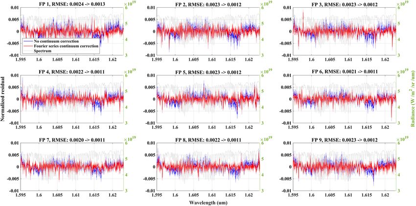
RESEARCH ARTICLE                           Toward High Precision XCO2 Retrievals From TanSat
10.1029/2020JD032794
                                           Observations: Retrieval Improvement and Validation
Key Points:
• First using O2 A and 1.61 um CO2
                                           Against TCCON Measurements
  band approaching TanSat XCO2
  retreival
                                           D. Yang1,2,3 , H. Boesch1,4 , Y. Liu2,3, P. Somkuti1,4,5 , Z. Cai2, X. Chen2, A. Di Noia1,4 ,
• Development a method on                  C. Lin6, N. Lu7, D. Lyu2, R. J. Parker1,4 , L. Tian8, M. Wang3 , A. Webb1,4, L. Yao2 , Z. Yin8,
  radiometric correction of TanSat         Y. Zheng6, N. M. Deutscher9, D. W. T. Griffith9 , F. Hase10, R. Kivi11 , I. Morino12 ,
  L1B data in O2 A and 1.61 um CO2
• Validation of new TanSat retrieval
                                           J. Notholt13 , H. Ohyama12 , D. F. Pollard14 , K. Shiomi15, R. Sussmann10, Y. Té16,
  against TCCON and recived                V. A. Velazco9 , T. Warneke13 , and D. Wunch17
  significant improved results
                                           1
  compare to previously retrieval           Earth Observation Science, School of Physics and Astronomy, University of Leicester, UK, 2Institute of Atmospheric
                                           Physics, Chinese Academy of Sciences, China, 3Shanghai Advanced Research Institute, Chinese Academy of Sciences,
Supporting Information:                    Shanghai, China, 4National Centre for Earth Observation, University of Leicester, UK, 5Colorado State University, Fort
• Supporting Information S1                Collins, CO, USA, 6Changchun Institute of Optics, Fine Mechanics and Physics, China, 7National Satellite Meteorological
                                           Center, China Meteorological Administration, China, 8Shanghai Engineering Center for Microsatellites, China, 9Centre
                                           for Atmospheric Chemistry, School of Earth, Atmospheric and Life Sciences, University of Wollongong, NSW, Australia,
                                           10
Correspondence to:                           Karlsruhe Institute of Technology, IMK‐IFU, Garmisch‐Partenkirchen, Germany, 11Space and Earth Observation
D. Yang,
                                           Centre, Finnish Meteorological Institute, Finland, 12National Institute for Environmental Studies (NIES), Tsukuba,
yangdx@mail.iap.ac.cn
                                           Ibaraki, Japan, 13Institute of Environmental Physics (IUP), University of Bremen, Bremen, Germany, 14National Institute
                                           of Water and Atmospheric Research Ltd (NIWA), Lauder, New Zealand, 15Japan Aerospace Exploration Agency, Japan,
Citation:                                  16
                                             Laboratoire d'Etudes du Rayonnement et de la Matière en Astrophysique et Atmosphères (LERMA‐IPSL), Sorbonne
Yang, D., Boesch, H., Liu, Y., Somkuti,    Université, CNRS, Observatoire de Paris, PSL Université, Paris, France, 17University of Toronto, Canada
P., Cai, Z., Chen, X., et al. (2020).
Toward high precision XCO2 retrievals
from TanSat observations: Retrieval
improvement and validation against         Abstract       TanSat is the 1st Chinese carbon dioxide (CO2) measurement satellite, launched in 2016. In
TCCON measurements. Journal of             this study, the University of Leicester Full Physics (UoL‐FP) algorithm is implemented for TanSat nadir
Geophysical Research: Atmospheres,         mode XCO2 retrievals. We develop a spectrum correction method to reduce the retrieval errors by the online
125, e2020JD032794. https://doi.org/
10.1029/2020JD032794                       fitting of an 8th order Fourier series. The spectrum‐correction model and its a priori parameters are
                                           developed by analyzing the solar calibration measurement. This correction provides a significant
Received 25 MAR 2020                       improvement to the O2 A band retrieval. Accordingly, we extend the previous TanSat single CO2 weak band
Accepted 24 JUL 2020                       retrieval to a combined O2 A and CO2 weak band retrieval. A Genetic Algorithm (GA) has been applied
Accepted article online 5 OCT 2020
                                           to determine the threshold values of post‐screening filters. In total, 18.3% of the retrieved data is identified as
                                           high quality compared to the original measurements. The same quality control parameters have been
                                           used in a footprint independent multiple linear regression bias correction due to the strong correlation with
                                           the XCO2 retrieval error. Twenty sites of the Total Column Carbon Observing Network (TCCON) have
                                           been selected to validate our new approach for the TanSat XCO2 retrieval. We show that our new approach
                                           produces a significant improvement on the XCO2 retrieval accuracy and precision when compared to
                                           TCCON with an average bias and RMSE of −0.08 ppm and 1.47 ppm, respectively. The methods used in this
                                           study can help to improve the XCO2 retrieval from TanSat and subsequently the Level‐2 data
                                           production, and hence will be applied in the TanSat operational XCO2 processing.

                                           1. Introduction
                                           Carbon Dioxide (CO2) has been recognized as the most important greenhouse gases causing climate change
                                           due to the rise in anthropogenic emissions since the industrial revolution. Accurate measurement of atmo-
                                           spheric CO2 in order to reduce the uncertainties of CO2 fluxes is a key requirement for meeting the “measur-
                                           able, reportable and verifiable” mitigation commitments of the United Nations Framework Convention on
©2020. The Authors.
This is an open access article under the   Climate Change (UNFCCC) (https://unfccc.int/resource/docs/2007/cop13/eng/06a01.pdf) that is aimed at
terms of the Creative Commons              avoiding disastrous consequences caused by climate change. The existing in‐situ surface CO2 measurement
Attribution License, which permits use,    networks provide a wealth of accurate data related to the global carbon cycle. Unfortunately, the sparse cov-
distribution and reproduction in any
medium, provided the original work is      erage of such networks is still a major limitation for global carbon cycle research and large uncertainties in
properly cited.                            our quantitative understanding of regional carbon fluxes remain.

YANG ET AL.                                                                                                                                               1 of 26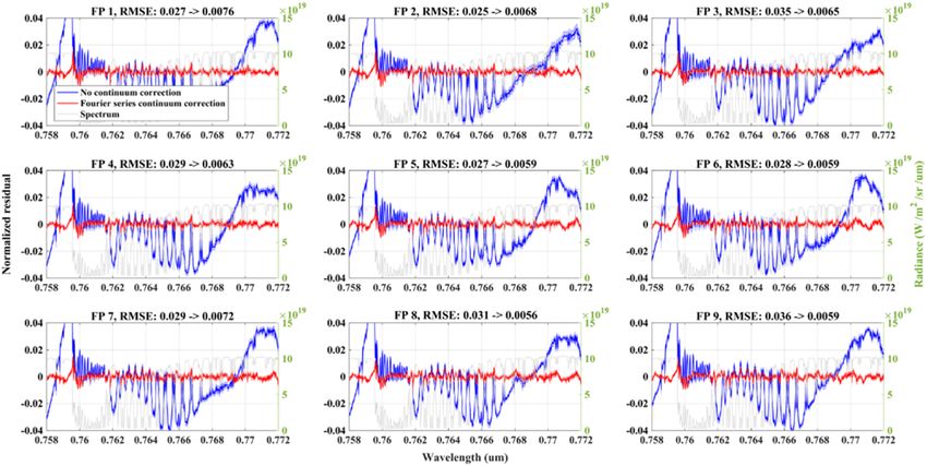
Journal of Geophysical Research: Atmospheres                                           10.1029/2020JD032794

                    The new generation of satellites with state‐of‐the‐art near infrared (NIR) and shortwave infrared (SWIR)
                    hyperspectral spectrometers bring us a step closer toward global mapping of CO2 with sufficient accuracy,
                    precision and coverage for reliable flux estimates on regional scales. Specifically, NIR/SWIR spectroscopy
                    provides a means for measurements of the total column‐averaged dry air CO2 mole fraction (XCO2) which
                    captures the CO2 signals in the lower troposphere including the boundary layer that can then be used to
                    improve our knowledge on CO2 surface fluxes (Kuang et al., 2002).
                    The European Space Agency (ESA) SCanning Imaging Absorption SpectroMeter for Atmospheric
                    CHartographY (SCIAMACHY) (Bovensmann et al., 1999) on board the ENVIronmental SATellite
                    (ENVISAT) that launched in 2002 and operated until 2012, was the first space‐borne instrument to provide
                    SWIR hyperspectral measurements of CO2 (Bösch et al., 2006; Buchwitz et al., 2005; Heymann et al., 2015;
                    Reuter et al., 2011), followed by the Greenhouse Gases Observing Satellite (GOSAT) from Japan (Kuze
                    et al., 2009) and the Orbiting Carbon Observatory‐2 (OCO‐2) from the U.S. (Crisp et al., 2008), launched
                    in 2009 and 2014, respectively. These missions have significantly contributed to the effort to obtain global
                    CO2 measurements from space (Eldering, O’Dell, et al., 2017; Yokota et al., 2009) and subsequently for car-
                    bon flux studies (Eldering, Wennberg, et al., 2017; Feng et al., 2017; Hakkarainen et al., 2016, 2019;
                    Maksyutov et al., 2013; Yang et al., 2017). When validated against measurements from the Total Carbon
                    Column Observing Network (TCCON) (Wunch, Toon, et al., 2011), XCO2 derived from GOSAT and
                    OCO‐2 has an accuracy of better than 2 part per million (ppm) (Butz et al., 2011; Buchwitz, Dils, et al., 2017;
                    Cogan et al., 2012; Crisp et al., 2012; Kim et al., 2016; O’Dell et al., 2012; Oshchepkov et al., 2013; Wu
                    et al., 2018; Yang et al., 2015; Yoshida et al., 2013), thanks to the high performance of these instruments
                    and long‐term calibration efforts (Crisp et al., 2017; Frankenberg et al., 2015; Kuze et al., 2014; Rosenberg
                    et al., 2016; Yoshida et al., 2013). Further advances are expected from recently launched missions such as
                    GOSAT‐2 (Nakajima et al., 2019) and OCO‐3 (Eldering et al., 2019) launched in 2018 and 2019 respectively,
                    and future missions including MicroCarb (Bertaux et al., 2020) and CO2M (Kuhlmann et al., 2019).
                    China plays an important role in the global carbon budget as a major source of anthropogenic carbon (Le
                    Quéré et al., 2018) due to its rapid economic development but also as a region of increased carbon sequestra-
                    tion thanks to a number of reforestation projects (Chen et al., 2019). In China, a series of ambitious projects
                    on mitigation of carbon emission was kicked‐off in the last 10 years, which include the first Chinese green-
                    house gas monitoring satellite mission (TanSat), which is supported by the Ministry of Science and
                    Technology of China, the Chinese Academy of Sciences, and the China Meteorological Administration.
                    The TanSat mission was initiated in 2011 and successfully launched on 22 Dec 2016. TanSat started acquir-
                    ing and archiving data operationally in March 2017 (Chen et al., 2012; Ran & Li, 2019).
                    TanSat carries two instruments on‐board: the Atmospheric Carbon Dioxide Grating Spectrometer (ACGS)
                    and the Cloud and Aerosol Polarimetry Imager (CAPI). ACGS is a state‐of‐the‐art hyperspectral grating
                    spectrometer aimed at allowing XCO2 retrievals (Lin et al., 2017; Liu et al., 2013; Wang et al., 2014) by mea-
                    suring backscattered sunlight in three NIR/SWIR bands: the oxygen (O2) A‐band (758–778 nm with
                    ~0.04 nm spectral resolution), the CO2 weak band (1,594–1,624 nm with ~0.125 nm spectral resolution)
                    and the CO2 strong band (2042–2082 nm with ~0.16 nm spectral resolution). CO2 column information is lar-
                    gely drawn from the weak CO2 band which includes a series of strong but not saturated CO2 lines which
                    respond to even small variations in atmospheric CO2 (Bösch et al., 2006; Kuang et al., 2002). The O2 A band
                    hyperspectral measurement contains information on aerosol and cloud scattering both in total scattering
                    amount and scattering vertical distribution (Corradini & Cervino, 2006; Geddes & Bösch, 2015; Heidinger
                    & Stephens, 2000). The strong CO2 band provides information on aerosol and cloud scattering at longer
                    wavelengths, in conjunction with information on CO2 and water vapor (Wu et al., 2019). The CAPI is a
                    multi‐band imager which provides radiance measurements in five bands (365‐408 nm, 660‐685 nm, 862‐
                    877 nm, 1,360‐1,390 nm, 1,628‐1,654 nm) from UV to NIR. In order to achieve more information on aerosol
                    size, which has a significant impact on the wavelength dependence of aerosol optical properties, CAPI
                    includes two polarization channels (660‐685 nm and 1,628‐1,654 nm) to measure the Stokes parameters
                    (Chen, Yang, et al., 2017).
                    TanSat flies in a sun‐synchronous low Earth orbit (LEO) with an equator crossing time around 13:30 local
                    time. The satellite operates in three measurement modes: nadir (ND), glint (GL) and target (TG). GL pro-
                    vides routine measurements over oceans which are obtained by tracking the principle plane (the principal

YANG ET AL.                                                                                                                 2 of 26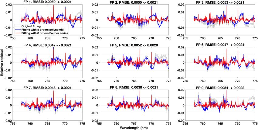
Journal of Geophysical Research: Atmospheres                                             10.1029/2020JD032794

                    plane is spanned by the vectors from the sun to the surface footprint and from the surface point to the obser-
                    ver). ND provides the routine measurements over land with the satellite flying in consistent rotation angle
                    routine as in GL mode. We only use ND observations in this study. The swath width of TanSat measure-
                    ments is ~18 km across the satellite track and contains 9 footprints each with a size of 2 km × 2 km in nadir
                    (Lin et al., 2017; Zhang et al., 2019). Nadir and glint mode alternate orbit‐by‐orbit, and the TanSat nadir
                    model ground track is typically between two OCO‐2 tracks, which provides potential future opportunities
                    for combined usage of both data products for increased spatial coverage.
                    The first global XCO2 dataset from TanSat observations for the first half year of operations has been pro-
                    duced with the Institute of Atmospheric Physics Carbon dioxide retrieval Algorithm for Satellite measure-
                    ment (IAPCAS) (Yang et al., 2018), using the CO2 weak band only. The nadir XCO2 dataset has been
                    evaluated using eight TCCON sites to show an average precision of 2.11 ppm for the TanSat retrievals
                    (Liu et al., 2018).
                    In this study, we apply the University of Leicester Full Physics (UoL‐FP) algorithm to the TanSat XCO2
                    retrieval using a joint CO2 weak band and O2 A band retrieval, after adopting a new approach to radiome-
                    trically correct TanSat spectra. This new radiometric correction is introduced in Section 2 together with the
                    UoL‐FP TanSat retrieval approach. The applied quality filtering and bias correction methods are discussed in
                    Section 3. Section 4 gives the results of the comparisons of the TanSat XCO2 retrievals to ground‐based obser-
                    vations from the TCCON network and Section 5 provides the summary and outlook.

                    2. UoL‐FP TanSat XCO2 Retrieval Description
                    2.1. Introduction of the UoL‐FP Algorithm
                    The UoL‐FP is an XCO2 retrieval algorithm based on the Optimal Estimation Method (OEM) that has been
                    originally developed for the NASA Orbiting Carbon Observatory (OCO) mission (Bösch et al., 2006), and has
                    been extensively used for XCO2 retrievals from GOSAT (Cogan et al., 2012). Besides XCO2, the UoL‐FP has
                    been used to retrieve methane (CH4) (Parker et al., 2011, 2015), HDO and H2O (Boesch et al., 2013) and Solar
                    Induced chlorophyll Fluorescence (Somkuti et al., 2020). UoL‐FP is also one of the algorithms used to gen-
                    erate the Essential Climate Variables (ECV) XCO2 and XCH4 from GOSAT for the ESA Climate Change
                    Initiative (CCI) (Buchwitz, Dils, et al., 2014 2017;) and subsequent European Commission Copernicus
                    Climate Change Service (C3S) (Buchwitz, Reuter, et al., 2017).
                    Several publications have already introduced the UoL‐FP algorithm and its applications in detail (Boesch et
                    al., 2013; Cogan et al., 2012; Parker et al., 2011) and here we only provide a brief overview. Basically, the
                    retrieval aims to resolve an optimization problem to find the best estimate of a state vector b x by minimizing
                    the difference between a measured and a simulated spectrum taking into consideration additional con-
                    straints on the measurement errors and state vector a priori uncertainties. This state vector gives all retrieved
                    parameters and includes atmospheric, surface and instrument variables. Full physics refers to the fact that
                    the algorithm generates the simulated spectrum via an accurate multiple‐scattering Radiative Transfer
                    (RT) model. As many processes involved in the transfer of light through the atmosphere respond in a
                    non‐linear way to changes in state vector elements, an iterative Levenberg–Marquardt (L‐M) inversion
                    scheme is used in the retrieval,
                                                                        −1  T −1
                                    x iþ1 ¼ x i þ ð1 þ λÞS−1    T −1
                                                          a þ K i Sε K i     K i Sε ðy − F ðx i ÞÞ−S−1
                                                                                                     a ðx i − x a Þ ;             (1)

                    where xa is the a priori of the state vector. Sa and Sε indicate the covariances of the state vector and the
                    measurement respectively. The weighting function (known as Jacobians) K gives the linear change of the
                    spectrum per change in state vector ∂y/∂x. The update step of the state vector’s ith iteration from xi to xi+1
                    can be adjusted by the L‐M factor λ.
                    The forward model, which includes a vector RT model, is one of the most essential parts of the retrieval algo-
                    rithm. In UoL‐FP, the radiative transfer model LIDORT is used, which is a linearized discrete ordinate radia-
                    tive transfer model that generates radiances and Jacobians simultaneously (Spurr et al., 2001; Spurr &
                    Christi, 2014). According to the instrument design, ACGS/TanSat only measures one direction of polarized
                    light instead of the total intensity; hence we need to compute the Stokes vector {I, Q, U, V} (Liou, 2002;

YANG ET AL.                                                                                                                  3 of 26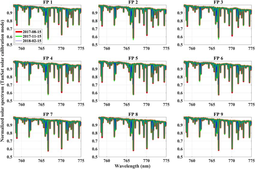
Journal of Geophysical Research: Atmospheres                                             10.1029/2020JD032794

                    Mishchenko et al., 2004; Stokes, 1852) in the forward simulation. Since multiple scattering is depolarizing, it
                    is reasonable to expect that the polarization could be accounted for by a low‐order scattering approximation.
                    For a relatively clear atmosphere (e.g. aerosol optical depth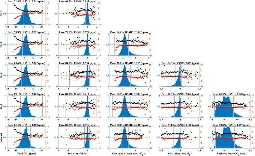
Journal of Geophysical Research: Atmospheres                                                      10.1029/2020JD032794

Figure 1. Mean spectrum of the normalized solar calibration measurement of the O2 A band. The average is calculated for each calibration measurement in an
orbit. Red, green and blue indicate the mean measurement taken for 2017/08/15, 2017/11/15 and 2018/02/15 respectively. Sub‐figures represent the footprints
(FP1–9) across the swath. The date is shown in the legend of FP1 sub‐figure.

                                      spectral calibration applied to a measured spectrum if an accurate solar model is used and the reflection from
                                      the diffuser is well known (Wang et al., 2018).
                                      Here, we use the new solar line model (2016 version) created by G. C. Toon (2014) (https://mark4sun.jpl.
                                      nasa.gov/toon/solar/solar_spectrum.html) combined with the UoL‐FP solar continuum model that is
                                      obtained from a polynomial fitting of SOLar SPECtrometer (SOLSPEC) measurements (Meftah et al., 2018).
                                      The solar line model has been extensively used and verified with GOSAT and OCO‐2 retrievals (Uchino
                                      et al., 2012). This solar model combines the solar lines and solar continuum, and hence can be directly used
                                      for solar model fitting without any further calculation.
                                      TanSat observes the Sun though a reflective diffuser before the relay optical system, hence the
                                      wavelength‐dependent diffuser reflectance needs to be compensated for, otherwise it could cause an extra
                                      pattern in the measured solar spectrum. In this study, we use a wavelength‐dependent Bidirectional
                                      Reflectance Distribution Function (BRDF) that has been characterized pre‐flight in the laboratory (Wang
                                      et al., 2014) without any corrections for a time dependent degradation as the instrument performance is
                                      stable. The solar irradiance is non‐polarized and we use a factor of 0.5 to adjust for the linear polarizer.
                                      To avoid contamination of terrestrial absorption from the upper atmosphere when the satellite observes the
                                      limb measurement region, only measurements with boresight solar zenith angle (defined angle between line
                                      of sight and solar) between 5° and 6° are used in fitting. Note that TanSat rotates by a 5° pitch angle (away
                                      from the Earth) to avoid damage of CAPI from strong incident light (Chen, Yang, et al., 2017; Chen, Wang,
                                      et al., 2017).
                                      2.3.2. Solar Calibration Analysis and Radiometric Corrections
                                      Monitoring the solar calibration spectrum shows a stable instrument performance during the first year of
                                      TanSat operations (Figure 1, the CO2 weak band is also stable but this is not shown here). The mean

YANG ET AL.                                                                                                                                       5 of 26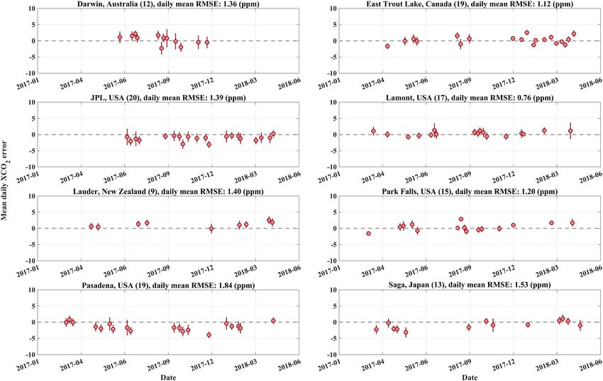
Journal of Geophysical Research: Atmospheres 10.1029/2020JD032794
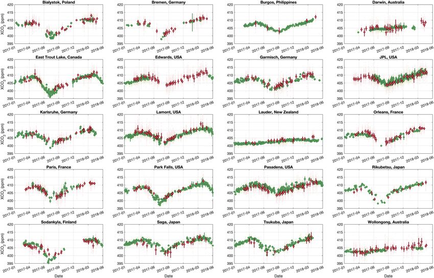
Figure 2. Mean fitting residuals of the solar calibration measurements. The average is calculated from the fitting residuals of 181,232 individual spectra (for each
th th
footprint, the quantity is ~20,136) during mar. 2017 – May 2018. The blue and red lines show the mean residual obtained by fitting a 5 order polynomials or a 8
order Fourier series model, respectively (see the detail in text section 2.3). The light gray line is the fitting residual when fitting a scale factor without any
wavelength dependent corrections. Sub‐figures indicate the 9 footprints (FP1‐FP9) across the swath. The RMSE shown in the title of each sub‐figure shows the
improvement of the Fourier series model compared to using the wavelength‐independent scale factor.
normalized solar measurement in the 750 nm region shows little change (mean normalized spectrum
changes < 0.1%) for spectra acquired every 3 months, except for a very small difference for solar lines,
which is probably caused by small instrument performance changes, e.g. instrument line shape (ILS). The
figure shows that spectra acquired for the different cross‐track footprints show some differences to each
other in the continuum, which means each footprint has to be analyzed separately.
In order to further investigate the solar calibration spectrum, we developed a fitting tool for the solar spec-
trum based on the solar model corrected for the variable Earth‐Sun distance and the Doppler shift effect (in
wavelength) due to Earth’s rotation and revolution. The fitting tool retrieves the wavelength dependence
continuum correction in different forms (e.g. polynomial or Fourier series) as well as a wavelength shift
and stretch simultaneously. The fitting tool uses the Gaussian‐Newton method without the constraint of
measurement noise.
The fitting algorithm is fast and hence we fit all individual solar spectra between March 2017 and May 2018
without averaging or manual spectrum selection. In total, 181,232 retrievals have been carried out and we
find consistent fitting residuals for each cross‐track footprint, which is expected considering the stable solar
calibration measurement (Figure 1). Averaged relative fitting residuals for the NIR band are given in
Figure 2. A considerable and consistent pattern with a mean RMSE of 0.48% remained in the fitting residual
when we only adjust a wavelength‐independent scaling factor to the continuum, which needs to be corrected
to avoid errors in the XCO2 retrieval. Thus, a method is needed that can compensate for these structures and
improve the fitting residual. However, this pattern is not a simple linear or quadratic function with wave-
length and a more complex model is needed. We found that the relative residual did not change much with
changes in intensity of the incident light introduced by instrument degradation and Earth‐Sun distance
changes and hence we adopt a correction model based on multiplicative continuum scaling rather than a
model using additive offsets.
YANG ET AL. 6 of 26
Journal of Geophysical Research: Atmospheres                                             10.1029/2020JD032794

                    A common approach is to use a polynomial as a function of wavelength to scale the continuum (Linc). We
                    have found that a 5th order polynomial is the best choice,

                                                                 5
                                                       L ¼ ∑i¼0 ai · Δλi · Linc þ DðλÞ;                                 (3)

                    where ai is the coefficient of the ith order of the polynomial component for a wavelength relative
                    (Δλ = λ − λ0, λ0 is the reference wavelength, in this study, we use first wavelength grid point of each band)
                    to a reference of 750 nm. D(λ) represents an additive offset assumed to be a linear function given by a
                    slope and a constant. This additive offset could compensate the impact from SIF (only O2 A band) and
                    stray light. As can be seen in Figure 2, this polynomial approach leads only to minor improvements in
                    the fitting residual. Increasing the order of the polynomial did not lead to significant improvements com-
                    pared to the 5th order.
                    An alternative approach that should have a better capability to capture the oscillating nature of the fitting
                    residuals is to use a Fourier series:
                                                    n
                                         L ¼ c þ ∑i¼1 ðai · cosði · ω · ΔλÞ þ bi · sinði · ω · ΔλÞÞ · Linc þ DðλÞ;            (4)
                    where ai and bi are coefficients of ith order of the Fourier series cosine and sine components with c being the
                    zero‐order coefficient, and ω the scaling coefficient for frequency. Δλ and D(λ) are the same as for the poly-
                    nomial model above. We have tested a 5th to 10th order Fourier series in the solar calibration fitting and
                    finally found that a 8th order is the best choice, which is because less than 8th order is not sufficiently com-
                    pensating the fitting residual and more than 8 leads to limited further improvement compared to 8th orders.
                    As a result of using Fourier series model, we find a significant improvement in the fitting residual with a
                    mean RMSE of 0.21% (Figure 2) compared to 0.48% for the polynomial approach. Note that, (1) the fitting
                    residual near solar lines is still larger than the measurement noise, and (2) a gas absorption structure is visi-
                    ble in the residuals, which is also the case in fit residuals for the CO2 weak band. This could be correlated
                    with stray light from Earth or preflight calibration (e.g. ILS and radiometric calibration), but the exact reason
                    is unclear and needs to be further investigated in the future. In principal, the continuum correction corrects
                    the dominant effects in the fitting residual but some features still remain visible in the residuals. For exam-
                    ple, larger residual structures appear for solar lines. Considering that this affects only a small number of pix-
                    els throughout a spectral band, it can be expected that impact on the retrieval is limited and we do not
                    attempt to further correct these features. This continuum feature is probably caused by several reasons, e.
                    g. radiometric calibration and stray light. For nadir observation, the component of incident light is more
                    complicated than for solar calibration due to the scattering and absorption in atmosphere. However, we
                    found similar residual features in both non‐corrected solar calibaration and nadir observation fitting.
                    Therefore, the applied Fourier series is applicable to nadir observation. But the parameters change between
                    solar calibration and nadir observation fitting and also among the soundings, and hence we retrieve all
                    Fourier series parameters in the cloud screening and XCO2 retrieval (See details in Text S3, Table S2 and
                    Figure S6, S7of SI).
                    The applied continuum correction in our study is basically a correction of the radiometric gain and no other
                    corrections are applied. This is because (1) errors of the continuum are more obvious and they are stable in
                    the case of TanSat, (2) solar lines are not sufficiently deep to constrain potential non‐linearity corrections, (3)
                    the ILS cannot be easily re‐analyzed from space‐based data, especially since TanSat did not provide solar
                    calibration measurement for the entire dayside which would scan the ILS due to the Doppler shift (Sun
                    et al., 2017).
                    2.4. O2 A Band Surface Pressure Retrieval for Cloud Screening
                    The O2 A band is important in the XCO2 retrieval because, (1) it allows cloud screening based on apparent
                    surface pressure to remove measurements that are highly contaminated by thick cloud, and (2) to provide
                    information on aerosol and thin clouds in a joint O2 A and CO2 band retrieval to reduce errors that are other-
                    wise introduced by light path modification from scattering.
                    An Oxygen A‐Band (ABO2) cloud‐screening algorithm is used as the cloud screening algorithm based on the
                    analysis of a small number of micro‐windows in the O2 A band. The ABO2 algorithm has been applied to
                    GOSAT and OCO‐2 cloud screening and verified against MODIS and CALIOP measurement (Taylor
                    et al., 2012, 2016). Unfortunately, the continuum correction described above cannot easily be applied to a

YANG ET AL.                                                                                                                   7 of 26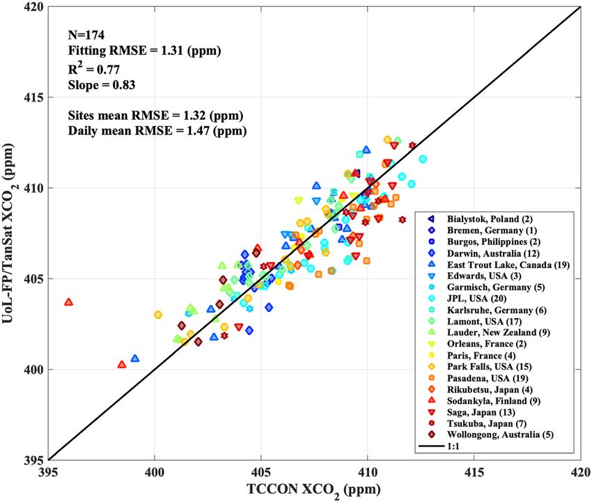
Journal of Geophysical Research: Atmospheres                                                          10.1029/2020JD032794

Table 1
List of state vector elements and descriptions for the UoL‐FP/TanSat retrieval
Acronym                                           Description                           N               A priori                          A priori error (1σ)

CO2 profile           Carbon dioxide (CO2) concentration on each layer surface           21   LMDZ MACC‐II CO2 model
                                                                                                                              p  ffiffiffiffiffiffi
H2O scale            Scaling for water vapor (H2O) profile                                1   ECMWF interim 0.75°               2
                                                                                                                                 0:1
                                                                                                                              p  ffiffiffiffiffi
Temperature shift    Shift for temperature profile                                        1   ECMWF interim 0.75°               2
                                                                                                                                 10 K
P surf               Surface pressure                                                    1   ECMWF interim 0.75°              2 hPa
Albedo B1            Surface albedo of oxygen (O2) A band                                1   Estimate from spectrum           1
                                                                                               continuum level
Albedo B1S           Surface albedo wavelength dependence slop of O2 A band             1    0                                0.0042
Albedo B2            Surface albedo of CO2 weak band                                    1    Estimate from spectrum           1
                                                                                               continuum level
Albedo B2S           Surface albedo wavelength dependence slope of CO2 weak band         1   0                                0.01
Aerosol M1           The profile of the most dominant aerosol type                       21   Copernicus Atmosphere
                                                                                               Monitoring Service (CAMS)
                                         nd
Aerosol M2           The profile of the 2      dominant aerosol type                     21   Copernicus Atmosphere
                                                                                               Monitoring Service (CAMS)
Cirrus               The profile of cirrus                                               21
Zeroff B1            The zero offset of O2 A band                                        1   0                                1% of continuum (SIF signal)
Zeroff B1S           The zero offset wavelength dependence slope of O2 A band            1   0                                1
Zeroff B2            The zero offset of CO2 weak band                                    1   0                                10% of continuum level
Zeroff B2S           The zero offset wavelength dependence slope of CO2 weak band        1   0                                1
Continuum B1         Fourier series correction coefficients on continuum of O2 A band,   17   Fitting results from long term   Comes from experimental value
                       1 frequency scale and 16 coefficients of trigonometric function          solar calibration
                                                                                               measurement
Continuum B2         Fourier series correction coefficients on continuum of CO2 band,    17   Fitting results from long term   Comes from experimental value
                       1 frequency scale and 16 coefficients of trigonometric function          solar calibration
                                                                                               measurement
Dispersion B1        Polynomials on wavelength grid for dispersion of O2 A band         6    L1B data, dispersion             Fixed with experimental value
                                                                                               coefficients O2 A
Dispersion B2        Polynomials on wavelength grid for dispersion of CO2 weak band     6    L1B data, dispersion             Fixed with experimental value
                                                                                               coefficients CO2 weak

                                        retrieval that uses narrow micro‐windows, and benefit from the fast RT model. Hence, we adopt an apparent
                                        surface pressure retrieval (assuming aerosol‐free conditions) based on a fast RT model for the whole range of
                                        the O2 A band (0.757–0.772 μm) that covers a multitude of O2 lines and continuum for both sides of the band.
                                        This retrieval includes surface pressure, temperature profile offset, Lambertian surface albedo and its
                                        wavelength dependence slope, wavelength stretch and the coefficients of the Fourier series continuum
                                        model in the NIR as retrieved parameters. The outputs are used later as a priori values for a subsequent
                                        XCO2 retrieval (Table 1). A priori surface pressure is taken from the European Centre for Medium‐Range
                                        Weather Forecasts (ECMWF) ERA‐Interim 0.75° × 0.75° reanalysis data product (Dee et al., 2011), and is
                                        interpolated to the location of the sounding and corrected for elevation differences using the U.S.
                                        Geological Survey’s (USGS) EROS Data Center Shuttle Radar Topography Mission Global 30 Arc‐Second
                                        Elevation (SRTM30) digital elevation model (DEM) (ftp://edcsgs9.cr.usgs.gov/pub/data/srtm/SRTM30).
                                        We found that the frequency coefficient (ω in equation (8)) of the Fourier series cannot be well‐fitted in the
                                        O2 surface pressure retrieval if the first guess is not very close to the true value due to non‐linear effects. Since
                                        we observe that the structure in the fitting residuals of the solar spectra changes little with time we can
                                        obtain a good first guess from the fitting of solar calibration measurement value, not only for ω but also
                                        for other coefficients. A set of 20,000 high quality solar calibration soundings (RMSE < 0.21%, which is
                                        the mean RMSE of all retrievals) including all 9 footprints have been selected for this calculation.
                                        Another highly non‐linear parameter is the stretch of the wavelength grid. The update of TanSat L1B data
                                        from version 1 to version 2 significantly improved the wavelength calibration, but additional corrections
                                        are still necessary. The solar calibration fitting also simultaneously provides wavelength stretch coefficients
                                        which we then use in the O2 A band surface pressure retrieval.
                                        The impact of the Fourier continuum correction on the surface pressure retrieval is significant (Figure 3).
                                        We found that (1) the retrieval without the correction has a large bias and scatter, and (2) there are large

YANG ET AL.                                                                                                                                                     8 of 26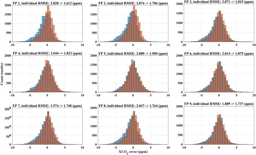
Journal of Geophysical Research: Atmospheres                                                        10.1029/2020JD032794

Figure 3. Histograms of surface pressure changes (δP surf) from O2 A band retrievals with (blue) and without (orange) Fourier series continuum correction for
selected clear‐sky conditions (selected cases on 2017‐10‐08) overpass TCCON/Lamont (USA) site. The changes are calculated by subtracting the a priori
(height corrected surface pressure from ECMWF interim) from the retrieved apparent surface pressure. The sub‐figures show the footprints (FP1‐FP9) across the
swath. The retrieved apparent surface pressure with continuum correction still shows a small bias to the a priori, because the retrieval has been carried out
without any consideration of aerosol and cloud scattering (see the detail in text section 2.4).

                                       differences between the cross‐track footprints in the retrieval even after continuum correction (with a
                                       constant gain factor). Therefore, the application of the apparent surface pressure retrieval for cloud
                                       screening without continuum correction is problematic due to the different scatter and bias for different
                                       footprints which could mean that a large number of clear‐sky measurement will be screened out for some
                                       footprints. As is shown for the case given in Figure 3, the surface pressure values for the retrieval with
                                       continuum correction mostly fall in the range between −10 to 0 hPa which satisfies the commonly used
                                       criterion for cloud screening of −20 to +20 hPa. In contrast, the retrieval without correction spreads
                                       between −10 to −30 hPa.
                                       A ± 20 hPa threshold for cloud screening is reasonable and relatively loose, which means more data is
                                       allowed to pass the cloud screening. The benefit is obvious: we do not include aerosol and cloud scattering
                                       corrections in the apparent surface pressure retrieval, so that there will always be a small bias in the retrieved
                                       surface pressure which can become more significant for very dark surfaces (Figure 3).

                                       2.5. TanSat XCO2 Two‐Band Retrieval
                                       The information on CO2 volume mixing ratio (VMR) comes to a large extent from the 1.6 μm CO2 weak
                                       band, which means that a retrieval based on only the weak band can provide a relatively accurate result if
                                       the measurement scene is not impacted by aerosols or if perfect knowledge on aerosols is available.
                                       Unfortunately, both are not possible for real scenarios. The preliminary TanSat XCO2 retrieval (version
                                       1.0) has been created using the CO2 weak band only (Liu et al., 2018; Yang et al., 2018). An extremely strin-
                                       gent filter has been applied in post screening, and hence screens out a large number of retrievals. The data
                                       produced with this approach provides good information on the global CO2 distribution and trend but does
                                       not yield enough quantity or accuracy for reliable surface flux inversions.
                                       The O2 A band surface pressure retrieval with our newly developed continuum correction shows reliable
                                       results; hence we can extend the CO2 retrieval with confidence to use the O2 A and CO2 weak band together
                                       to improve the retrieval accuracy. We have applied a two‐band retrieval to produce XCO2 data from sound-
                                       ings that are recognized as clear‐sky scenes by the cloud screening. The retrieval uses a state vector that
                                       includes a CO2 profile, scale factors for temperature and water vapor, surface pressure, surface albedo and

YANG ET AL.                                                                                                                                          9 of 26
Journal of Geophysical Research: Atmospheres 10.1029/2020JD032794
Figure 4. Mean O2 A band fitting residuals (normalized by continuum level) from the two bands retrieval with (red) and without (blue) Fourier series continuum
correction. The average is computed from selected clear‐sky measurements on 08/10/2017 around the TCCON/Lamont site. The corresponding MODIS/aqua
RGB image is shown in Figure 3. The light gray line (right y‐axis) shows the measurement spectrum as reference. The red and blue shading indicates the
continuum normalized standard deviation (SD) for the retrieval with and without Fourier series continuum correction respectively.
spectral slope. In addition, we fit an additive zero offset and its wavelength dependent slope in both the O2 A
and CO2 weak bands. For the CO2 weak band, the same correction model as for the O2 A band is applied.
The full state vector is given in Table 1.
Significant improvements to the O2 A band residual have been found when using the Fourier series correc-
tion. The Standard Deviation (SD) of the normalized residual indicates that the fitting is stable (Figure 4).
Notice that the residuals of the 9 footprints show a slight difference even with the correction, e.g. at the
long‐wavelength end that contain few atmospheric absorption features, which means this correction cannot
perfectly compensate all of the spectral patterns. The residual still contains structures related to O2 lines,
which is because (1) the spectroscopy is not perfect (Connor et al., 2016), and (2) the observed residual fea-
tures for the solar calibration fitting which we discussed in section 2.3. The improvement for the CO2 weak
band is also large (Figure 5) and the RMSE is reduced by almost half for the retrieval with the continuum cor-
rection. Similar to the O2 A band, minor residual patterns remain and need to be investigated in the future.
3. Quality Control and Bias Correction
3.1. Dataset
To remove outliers and to correct for small biases, a quality control filter and bias correction is applied using
a reference dataset that is reliable enough for indicating retrieval errors. The Total Carbon Column
Observing Network (TCCON) provides accurate measurement of XCO2 (Wunch, Toon, et al., 2011;
Wunch et al., 2015), and has been used for GOSAT and OCO‐2 filtering and bias correction (Kim et al., 2016;
Oshchepkov et al., 2013; Wunch, Wennberg, et al., 2011; Wunch et al., 2017; Wu et al., 2018; Yoshida
et al., 2013). The OCO‐2 team has also developed additional methods for filtering and bias correction for
their version 8 product, including small area approximation, multi‐model median and southern hemisphere
approximation (O'Dell et al., 2018). In this study we only focus on the retrieval around TCCON sites, and
hence only the data of 20 TCCON sites (Table 2) has been selected as a reference dataset for bias/filtering
and validation in this study.
YANG ET AL. 10 of 26Journal of Geophysical Research: Atmospheres 10.1029/2020JD032794
Figure 5. Same as Figure 4, but for the CO2 weak band.
The quality control (filtering), bias correction and validation is based on an inter‐comparison of UoL‐FP/
TanSat retrievals against TCCON measurement, and those two results have been obtained from two differ-
ent instruments and retrieval algorithms with different averaging kernels and a priori assumptions. A
method for removing smoothing error differences caused by the different instruments and retrieval
Table 2
The TCCON site list used in the validation study and the site validation statistics
Date range Validation
Site N bias (ppm) RMSE (ppm)
Bialystok, Poland (Deutscher et al., 2019) 20,090,301–20,180,427 2 0.78 0.93
Bremen, Germany (Notholt et al., 2019) 20,070,115–20,180,420 1 −0.29 0.29
Burgos, Philippines (Morino, Velazco, et al., 2018; Velazco et al., 2017) 20,170,303–20,180,427 2 0.27 1.10
Darwin, Australia (Griffith, Deutscher, et al., 2014) 20,050,828–20,180,308 12 0.29 1.36
East Trout Lake, Canada (Wunch et al., 2018) 20,161,007–20,181,231 19 0.21 1.12
Edwards, USA (Iraci et al., 2016) 20,130,720–20,181,231 3 1.36 1.39
Garmisch, Germany (Sussmann & Rettinger, 2018a) 20,070,716–20,181,220 5 0.24 1.18
JPL, USA (Wennberg et al., 2014) 20,110,519–20,180,514 20 −1.12 1.39
Karlsruhe, Germany. (Hase et al., 2015) 20,100,419–20,190,121 6 0.33 1.67
Lamont, USA (Wennberg et al., 2016) 20,080,706–20,181,231 17 0.37 0.76
Lauder, New Zealand (Sherlock et al., 2014) 20,100,202–20,181,031 9 1.19 1.40
Orléans, France (Warneke et al., 2019) 20,090,829–20,180,405 2 1.40 1.83
Paris, France. (Té et al., 2014) 20,140,923–20,180,126 4 0.048 0.62
Park Falls, USA (Wennberg et al., 2017) 20,040,602–20,181,229 15 0.41 1.20
Pasadena, USA (Wennberg et al., 2015) 20,120,920–20,181,231 19 −1.41 1.84
Rikubetsu, Japan (Morino, Yokozeki, et al., 2018) 20,131,116–20,180,423 4 −0.85 1.12
a *
Sodankylä Finland (Kivi et al., 2014) 20,090,516–20,181,030 9 1.17 (0.35) 2.83 (1.25)
Saga, Japan (Shiomi et al., 2014) 20,110,728–20,181,021 13 −0.92 1.53
Tsukuba, Japan (Morino, Matsuzaki, et al., 2018) 20,110,804–20,180,427 7 −1.04 1.62
Wollongong, Australia (Griffith, Velazco, et al., 2014) 20,080,626–20,180,425 5 0.90 1.23
Zugspitze, Germany (Sussmann & Rettinger, 2018b) 20,150,424–20,181,218 ‐ ‐ ‐
a
Large bias point removed
YANG ET AL. 11 of 26Journal of Geophysical Research: Atmospheres 10.1029/2020JD032794
Table 3
Selected filter used in quality control and corresponding lower and upper thresholds
Name Description Lower boundary Upper boundary
Grad CO2 The retrieval changes of layer CO2 gradient between 700 hPa and the surface −4.34 21.47
Delta Psurf The retrieval changes on surface pressure from a priori −4.45 1.99
Continuum B1C3 Continuum correction coefficients of cos(x) of O2 A band −0.76 0.60
Zeroff B2S Zero offset wavelength dependence slope of CO2 band −0.14 0.017
AlbedoB2 Surface albedo of CO2 weak band 0.033 0.33
Zeroff B1S Zero offset wavelength dependence slope of O2 A band ‐ ‐
H2Oscale Scale factor of H2O ‐ ‐
Continuum B1C4 Continuum correction coefficients of sin(x) of O2 A band ‐ ‐
algorithm (Rodgers & Connor, 2003) has been used in GOSAT (Cogan et al., 2012) and OCO‐2 validation
(O'Dell et al., 2018; Wunch et al., 2017). In practice, the application of this correction has led to small
changes ofJournal of Geophysical Research: Atmospheres 10.1029/2020JD032794
retrieval for versions V7 (Wunch, Toon, et al., 2011), and in subsequent
versions V8 (O'Dell et al., 2018) and V9 (Kiel et al., 2019). In this study,
we hope to use a method that is less driven by empirical decisions. A
machine learning Genetic Algorithm (GA) method has been developed
and applied to OCO‐2 to generate warn level data (Mandrake et al., 2013).
The algorithm optimizes complexity (how many filters are selected),
threshold value and transparency (how many data points pass the filter,
represented by percentage) simultaneously. Mandrake et al. (2013) use
one additional species of gene to control the filter selection and optimize
this selection simultaneously, which treats each candidate equally, and
then causes the filter combination for each complexity to be different.
In this study, the filter has been selected according to the rank of the
δ xco2 correlation, which means that the selection of the filter combination
is carried out after the complexity is fixed. For each GA, runs with differ-
ent complexity from 2 to 8 are carried out and shown in Figure 6. We opti-
mize the threshold values of all filters for each GA run with chosen
complexity with different transparency simultaneously (see more details
Figure 6. The optimal target run genetic algorithm (GA) profile (Pareto‐ of the GA that is used in this paper in Appendix B).
optimal trade‐off curves) for the selection of filter complexity and
transparency. The XCO2 mean individual RMSE is a total RMSE calculated Subjective selection of transparency and complexity is required at the end
from all retrievals which pass the optimized threshold value (good of the applied GA. The transparency for different complexities against
retrieval). The color indicates the number of parameters (complexity) that RMSE is shown in Figure 6. It needs to be noted that for each complexity
are used in the GA run. For each complexity, the filter is determined and the filter is fixed, which means the complexity +1 represents the addition
fixed (see section 3.2.1 for details and Table 3 for filter definitions).
of an extra filter (Table 3). Few improvements on filter selection have
Transparency has a 1% interval through 0–100%. No significant additional
reduction in the RMSE was seen when using more than 5 filters. In this been found when the complexity is larger than 4 for the determination
study, we cut‐off at 2 ppm with 5 filters, which is an ad hoc choice, and the of OCO‐2 warn levels (Mandrake et al., 2013). We also found similar
transparency is 64.3%. The 2 ppm RMSE is a compromise between results for a complexity of 5 when compared to the complexity runs with
coverage and accuracy. The RMSE is calculated from individual TCCON values of 2–8 (Figure 6). The advantages of multi‐feature combinations for
overpass couples, which means the footprint can be spatially away from the
more than 4 features appears only when the fraction of filtered‐out data is
TCCON location, and hence there are would be geolocation differences
that casue naturally CO2 differences. In addition, we also have to consider close to 50%, and there are few advantages if the fraction of filtered‐out
the measurement error and bias that include in the RMSE. data becomes less than 30% (transparency > 70%). For a target of 2 ppm
RMSE, we select a transparency between 64–65% (64.3%) with five filters.
3.2.2. Application of the Filter
Retaining as much data as possible for a given requirement of RSME is an advantage of the GA method.
However, GA can give an optimal solution in a mathematical sense, which may not be physically reasonable;
namely the filter thresholds are unrealistic. For contrasting the results obtained with GA against manual selec-
tion, we also applied an empirical selection of filter thresholds for the five first filters applied in GA (Table 3).
The results are compared in Figure 7 using the bin‐error plot method which is similar to that used by O’Dell
et al. (2018) for OCO‐2 post screening. In general, we find that the thresholds from GA and the empirical
method (manual selection) have similar effects on the filtering. However, to achieve a similar RSME with the
empirical selection of thresholds, we reduce the amount filtered data by an additional 13.5% compared to GA.
Some filters, e.g. Grad CO2, Delta Psurf, and AlbedoB2, are parameters which have a specific physical mean-
ing. Although these parameters are constrained during the retrieval, unreasonable results still occasionally
occur. The GA that has been applied in this study has no capability of judging if a threshold has a reasonable
value or not. Therefore, in practice, we strongly recommend applying additional physical filters to remove
unreliable retrievals, if needed. However, in this study we only use GA screening.
In summary, our retrieval convergence rate is 94.8% of the cloud‐free measurement (~30% of the original
measurements for a 20 hPa threshold of the apparent surface pressure from the O2 A band) and 64.3% have
been recognized as good retrievals by GA. In total, we keep ~18.3% of all nadir measurements, and subse-
quently apply a bias correction to them.
3.3. Bias Correction
The bias correction is applied after the quality control. Biases in retrieved XCO2 can be introduced by
shortcomings in the retrieval algorithm (e.g. parameterized models and radiative transfer), the
YANG ET AL. 13 of 26Journal of Geophysical Research: Atmospheres 10.1029/2020JD032794
Figure 7. The performance of the GA with 2–5 filters (rows 1–4) and a manual filter threshold selection with 5 filters (row 5). The histograms (left y‐axis) indicate
the counts for each filter bin, and red and black solid points show the bias and RMSE for each bin (right y‐axis). The gray line is the upper and lower
threshold used for each filter. The filters are applied from left to right (columns 1–5) sequentially.
measurements (e.g. stray light or calibration) and the databases which are used (e.g. gas absorption and solar
model). The former two will typically lead to variable biases that will depend on other parameters while the
latter one more likely induces a global bias. Commonly, the parameter‐dependent bias dominates and can be
corrected (Wunch, Wennberg, et al., 2011) using a linear combination of identified bias parameters, ΔXCO2 ¼
n
∑i¼1 ai · pi þ b, with ai being the linear coefficient for the ith parameter pi, and b an offset.
For the bias correction, we use the filters that have already been applied in the quality control as these five
parameters are most strongly correlated with the error in XCO2. A multiple linear regression is applied to
find the coefficients ai for each across‐track footprint. A further small improvement in RMSE is found with
increasing the number of parameters up to 16 (SI section 1). The most significant improvement appears for
the first three parameters and further parameters have a smaller effect. Improvement becomes less signifi-
cant when using more than 12 parameters. Here, we use five parameters to avoid over‐optimizing the bias
correction. The number and selection of filter parameters is somewhat subjective and has been made to
agree with the quality control. Using rank of XCO2 individual error correlation to select bias correction para-
meters sometimes could miss bias correlated parameters, and hence more bias relative studies are recom-
mend in the next stage research. The bias mostly comes from imperfect forward model and measurement
(e.g. stray light and calibaration issue), and they mixed but independent for each footprint. The parameter
bias correction does not only involve physical parameters but also parameters used for the spectrum correc-
tion. Therefore, we perform the bias correction separately to each footprint.
The effect of the bias correction is shown in Figure 8. The largest improvements in RMSE are found for foot-
print 1, 2, 7, and 8. Besides a parameter‐related bias, there can also be a footprint dependent bias as has been
YANG ET AL. 14 of 26Journal of Geophysical Research: Atmospheres 10.1029/2020JD032794
Figure 8. The individual XCO2 error (UoL‐FP/TanSat against TCCON) change with and without parameter bias correction. The orange and blue histograms
indicate the XCO2 individual error distribution with and without bias correction. The improvement of RMSE with and without bias correction for each
footprint (FP 1–9) across the swath is shown in the titles.
shown for OCO‐2. Typically, a stable and constant bias mainly relates to instrument effects (O'Dell et
al., 2018; Wu et al., 2018). TanSat has 9 footprints in a swath across ~18 km on the ground on average. In
our retrieval, we also investigate the cross‐footprint bias by subtracting the mean value of a swath when
all 9 across‐track footprints are available. After the independent parameter bias correction, no obvious
cross‐track footprint bias is found and the average bias is less than 0.1 ppm but with a large (>0.3 ppm)
standard deviation (SD). This result is also true, when we select the swaths for low variation of surface
albedo across the swath (SD < 0.01) to guarantee that the scene is comparable through all footprints (only
532 swaths satisfy this criteria). This result indicates that parameter bias correction, if carried out for each
footprint independently, can reduce the across‐track bias.
4. XCO2 Retrievals Over TCCON Sites
4.1. The Discussions on Two‐Bands Retrieval
The Fourier series approach, introduced in section 2.3, has been instrumental in allowing a two‐bands retrie-
val that uses the O2 A band together with the weak CO2 band. As shown in section 2.3, the continuum cor-
rection for the O2 A band in the XCO2 retrieval leads to a significantly improved fitting residual for all 9
footprints. We have also found that the apparent surface pressure retrieval (sect.2.4) from the O2 A band
yields reliable results when adopting the continuum correction. In this study, we retrieve XCO2 from
TanSat nadir measurements from March 2017 to May 2018 around 20 TCCON sites (Table 2, and see detail
in sect.3.1) by using the setup that has been introduced in section 2.5. The continuum correction effect (as
discussed in sect.2.3) on XCO2 is shown in Figure 9 for TanSat retrievals around the TCCON/Lamont
(USA) site using all TanSat retrievals that pass the quality control but without bias correction. The RMSE
decreases from 4.08 ppm to 1.59 ppm, while the bias changes from 0.57 ppm to −0.56 ppm. We also found
that more retrievals fail to converge if no continuum correction is applied, meaning that the continuum
YANG ET AL. 15 of 26Journal of Geophysical Research: Atmospheres 10.1029/2020JD032794
Figure 9. Histogram of individual XCO2 retrieval errors (difference between TanSat and TCCON XCO2) for TCCON/
Lamont for clear‐sky measurements. The orange (right y‐axis) and blue (left y‐axis) give the results for the two‐band
retrieval with (orange) and without (blue) Fourier series continuum correction. All data statistics in this figure
passed quality control, but there is no bias correction applied. The RMSE remove bias shown in text box of this figure
gives the RMSE calculated from each individual error after subtracting the overall bias.
correction also improved the retrieval robustness. In summary, the continuum correction and usage of the
O2 A band shows a significant improvement on the retrieval precision. We also compared our new
approach with the TanSat XCO2 retrieval from a single CO2 band only (Figure 10). The single CO2 weak
band retrieval has been carried out with UoL‐FP/TanSat retrieving the CO2 profile, surface albedo and
wavelength stretch, assuming no aerosol and cloud scattering in the atmosphere. This is the same strategy
used by the IAPCAS (the Institute of Atmospheric Physics Carbon dioxide retrieval Algorithm for Satellite
remote sensing) retrieval to generate preliminary TanSat XCO2 data (Liu et al., 2018; Yang et al., 2018).
The improvement is significant both on the bias and RMSE. The bias is reduced by ~1 ppm, while the
RMSE decreases from 3.43 to 1.59 ppm.
Figure 10. Same as Figure 9, but for a comparison between a single CO2 weak band retrieval (no continuum correction)
and the two‐band retrieval with Fourier series continuum correction.
YANG ET AL. 16 of 26Journal of Geophysical Research: Atmospheres 10.1029/2020JD032794
Figure 11. Validation of UoL‐FP/TanSat XCO2 retrievals against measurements from 20 TCCON sites. Each symbol
represents the mean of one overpass (see detail in text section 3.1 for colocation criteria) for TanSat (only shown if
the available quantity N > 50) and the TCCON average during the overpass (only show if the available quantity N > 20).
The total number of overpasses per site is given in the legend. In total 174 TCCON overpasses are involved in this
validation. Statistics are shown in the upper‐left corner of the figure. The daily mean RMSE is the total RMSE computed
from each overpass mean and the site mean RMSE is computed by averaging the RMSE of each site. The black line
2
indicates the 1:1 line as reference. The slope, R and fitting RMSE are the statistics from a linear regression weighted by
bi‐square.
4.2. Validation Against TCCON Measurement
To compare TanSat retrievals to TCCON measurements, we average the quality‐controlled, bias‐corrected
TanSat retrievals per overpass including all across‐track footprints for a swath, as no obvious across‐track
footprint bias has been observed. Only overpasses with more than 50 soundings are used. Figure 11 shows
the comparisons of the TanSat XCO2 average per overpass compared to the TCCON retrievals averaged over
±1 hour of the overpass time. From the 174 data pairs found, we can infer a daily mean bias of 0.08 ppm and
a RSME of 1.47 ppm, which are parameters often used to characterize retrieval performance (Cogan
et al., 2012; O'Dell et al., 2018; Wu et al., 2018). The linear regression has a slope of 0.83 and R2 of 0.77.
However, these statistics can be misleading, as sites with large numbers of overpasses will have a larger
weight than sites with fewer overpasses, and therefore this average is dominated by the few sites with a large
number of overpasses. Consequently, the figure also displays the overall mean of the mean RMSE per site
with the individual values for mean bias and RMSE given in (Table 2).
Overall, we find that mean biases are small but show a noticeable variation between sites which is partly due
to the low number of data points at some sites. Considering only the seven sites with more than 10 over-
passes, we find that JPL (USA), Pasadena (USA) and Saga (Japan) show a large (~1 ppm) negative bias.
JPL (USA) and Pasadena (USA), for example, have a strong impact from the nearby city of Los Angles
(USA), and it is suggested not to include these sites for bias correction (O'Dell et al., 2018). The linear regres-
sion with a slope of 0.83 and R2 of 0.77 can be improved to 0.84 and 0.92 respectively by removing measure-
ments at Pasadena (USA), JPL (USA), Tsukuba (Japan) and Saga (Japan) (see SI section 2).
For the other four sites, Lamont, Park Falls, Darwin and East Trout Lake, we observe small biases of a few
tenths of a ppm only. For Lauder (New Zealand) and Sodankyla (Finland) we also observe large biases, but
YANG ET AL. 17 of 26You can also read