Consistent coupling of positions and rotations for embedding 1D Cosserat beams into 3D solid volumes - export.arXiv.org
←
→
Page content transcription
If your browser does not render page correctly, please read the page content below
manuscript No.
                                         (will be inserted by the editor)

                                         Consistent coupling of positions and rotations for embedding
                                         1D Cosserat beams into 3D solid volumes
                                         Ivo Steinbrecher · Alexander Popp · Christoph Meier
arXiv:2107.11151v1 [cs.CE] 23 Jul 2021

                                         Received: date / Accepted: date

                                         Abstract The present article proposes a mortar-type finite        ded mortar-type formulation for rotational and translational
                                         element formulation for consistently embedding curved, slen-      constraint enforcement denoted as full beam-to-solid volume
                                         der beams into 3D solid volumes. Following the fundamental        coupling (BTS-FULL) scheme. Based on elementary nu-
                                         kinematic assumption of undeformable cross-sections, the          merical test cases, it is demonstrated that a consistent spatial
                                         beams are identified as 1D Cosserat continua with point-          convergence behavior can be achieved and potential locking
                                         wise six (translational and rotational) degrees of freedom        effects can be avoided, if the proposed BTS-FULL scheme
                                         describing the cross-section (centroid) position and orienta-     is combined with a suitable solid triad definition. Eventually,
                                         tion. A consistent 1D-3D coupling scheme for this problem         real-life engineering applications are considered to illustrate
                                         type is proposed, requiring to enforce both positional and        the importance of consistently coupling both translational
                                         rotational constraints. Since Boltzmann continua exhibit no       and rotational degrees of freedom as well as the upscal-
                                         inherent rotational degrees of freedom, suitable definitions      ing potential of the proposed formulation. This allows the
                                         of orthonormal triads are investigated that are representative    investigation of complex mechanical systems such as fiber-
                                         for the orientation of material directions within the 3D solid.   reinforced composite materials, containing a large number
                                         While the rotation tensor defined by the polar decomposi-         of curved, slender fibers with arbitrary orientation embedded
                                         tion of the deformation gradient appears as a natural choice      in a matrix material.
                                         and will even be demonstrated to represent these material
                                                                                                           Keywords Beam-to-solid coupling · 1D-3D position and
                                         directions in a L2 -optimal manner, several alternative triad
                                                                                                           rotation coupling · Mixed-dimensional coupling · Finite
                                         definitions are investigated. Such alternatives potentially al-
                                                                                                           element method · Geometrically exact beam theory · Mortar
                                         low for a more efficient numerical evaluation. Moreover, ob-
                                                                                                           methods · Fiber-reinforced materials
                                         jective (i.e. frame-invariant) rotational coupling constraints
                                         between beam and solid orientations are formulated and en-
                                         forced in a variationally consistent manner based on either       1 Introduction
                                         a penalty potential or a Lagrange multiplier potential. Even-
                                         tually, finite element discretization of the solid domain, the    Embedding fibers or beams, i.e. solid bodies that can me-
                                         embedded beams, which are modeled on basis of the geomet-         chanically be modeled as dimensionally reduced 1D struc-
                                         rically exact beam theory, and the Lagrange multiplier field      tures since one spatial dimension is much larger than the
                                         associated with the coupling constraints results in an embed-     other two, into a 3D matrix material is a common approach
                                                                                                           to enhance the mechanical properties of a structure. Fiber-
                                         I. Steinbrecher, A.Popp                                           reinforced structures can be found in many different fields,
                                         Institute for Mathematics and Computer-Based Simulation,          e.g. in form of steel reinforcements within concrete struc-
                                         University of the Bundeswehr Munich,
                                         Werner-Heisenberg-Weg 39, D-85577 Neubiberg, Germany
                                                                                                           tures, lightweight fiber-reinforced composite materials based
                                         E-mail: ivo.steinbrecher@unibw.de                                 on carbon, glass or polymer fibers in a plastic matrix, or ad-
                                         C. Meier
                                                                                                           ditively manufactured components allowing for a very flex-
                                         Institute for Computational Mechanics,                            ible and locally controlled reinforcement of plastic, metal,
                                         Technical University of Munich,                                   ceramic or concrete matrix materials [32, 33, 42]. At a dif-
                                         Boltzmannstrasse 15, D-85748 Garching b. München, Germany         ferent length scale, fiber embeddings play a key role for
2                                                                                                               Ivo Steinbrecher et al.

essential processes in countless biological systems, e.g. in        61], which is known to combine high model accuracy and
the form of embedded networks (e.g. cytoskeleton, extracel-         computational efficiency [5, 53]. Based on the fundamental
lular matrix, mucus) or bundles (e.g. muscle, tendon, liga-         kinematic assumption of undeformable cross-sections, such
ment) [2, 21, 31, 41]. Most of these applications are charac-       beam models can be identified as 1D Cosserat continua with
terized by geometrically complex embeddings of arbitrarily          six degrees of freedom defined at each centerline point to
oriented, slender and potentially curved fibers. Computa-           describe the cross-section position (three translational de-
tional models predicting the response of such reinforced            grees of freedom) and orientation (three rotational degrees
structures are essential for a time- and cost-efficient de-         of freedom). Thus, the problem of beams embedded in a
sign and development of technical products, but also to gain        3D solid volume can be classified as mixed-dimensional 1D-
fundamental understanding of biological systems at length           3D coupling problem between 1D Cosserat continua and a
scales that are not accessible via experiments. In the context      3D Boltzmann continuum. A variety of 1D-3D coupling ap-
of computational modeling, as considered in the following,          proaches exist in the literature, however most of them involve
the embedded 1D structures will be referred to as fibers or         truss / string models, i.e. 1D structural models account only
beams, respectively, and the 3D matrix as solid.                    for internal elastic energy contributions from axial tension,
     One common modeling approach for this physical beam-           e.g. [13, 17, 20, 25, 26, 43, 50]. Work on the 1D-3D cou-
to-solid volume coupling problem is based on homogenized,           pling between beams, i.e. full Cosserat continua, and solids
anisotropic material models for the combined fiber-matrix           is much rarer. In [16], collocation along the beam center-
structure [1, 70]. This widely used approach is appealing           line is applied to couple beams with a surrounding solid
since, e.g. no additional degrees of freedom are required to        material. A mortar-type coupling approach is proposed in
model individual fibers, and existing simulation tools can be       the authors’ previous work [63], where a Lagrange multi-
used as long as they support anisotropic material laws. How-        plier field is defined along the beam centerline to weakly
ever, such models cannot give detailed information about            enforce the coupling constraints. The 1D-3D coupling be-
the interactions between fibers and surrounding matrix as,          tween beams and a surrounding fluid field, as relevant for
e.g. required to study mechanisms of failure. Moreover, the         fluid-structure-interaction (FSI) problems, has been consid-
fiber distribution in the solid has to be sufficiently homoge-      ered in some recent contributions [22, 68].
neous and a separation of scales is required, i.e. the fiber size        All the aforementioned 1D-3D beam-to-solid coupling
has to be sufficiently small as compared to the smallest di-        schemes have in common that only the beam centerline po-
mension of the overall structure. Eventually, when modeling         sitions, but not the cross-section orientations, are coupled
new fiber arrangements, the homogenization step inherent            to the solid, which will be denoted as translational 1D-3D
to these continuum models requires sub-scale information,           coupling. In such models, an embedded fiber can still per-
e.g. provided by a model with resolved fiber geometries.            form local twist/torsional rotations, i.e. cross-section rota-
     Another modeling approach consists of fully describing         tions with respect to its centerline tangent vector, relative to
the fibers and surrounding solid material as 3D continua.           the solid. While this simplified coupling procedure can rea-
This leads to a surface-to-surface coupling problem at the          sonably describe the mechanics of certain problem classes
2D interface between fiber surface and surrounding solid. In        where such relative rotations will rarely influence the global
the context of the finite element method, these surfaces can be     system response, e.g. embedding of straight fibers with cir-
tied together by either applying fiber and solid discretizations    cular cross-section shape, for most practical applications a
that are conforming at the shared interface or via interface        more realistic description of the physical problem requires
coupling schemes accounting for non-matching meshes, such           to also couple the rotations of beam and solid.
as the mortar method [45, 47–49]. Alternatively, extended               In a very recent approach by [27] the full 1D-3D cou-
finite element methods (XFEM) [40] or immersed finite el-           pling problem involving positions and rotations has been ad-
ement methods [29, 55] can be used to represent 2D fiber            dressed for the first time. The coupling of the two directors
surfaces embedded in an entirely independent background             spanning the (undeformable) beam cross-section with the
solid mesh. While such fully resolved modeling approaches           underlying solid continuum together with the coupling of
allow to study local effects with high spatial resolution, the      the cross-section centroids results in a total of nine coupling
significant computational effort associated with these mod-         constraints. One specific focus of this interesting contribution
els prohibits their usage for large-scale systems with a large      lies on a static condensation strategy, which allows to elim-
number of slender fibers.                                           inate the associated Lagrange multipliers and the beam bal-
     The class of applications considered here typically in-        ance equations from the final, discrete system of equations.
volves very slender fibers. In this regime it is well justified,    The requirement of a C 1 -continuous spatial discretization of
and highly efficient from a computational point of view, to         the solid domain, as resulting from the proposed condensa-
model individual fibers as beams, e.g. based on the geometri-       tion strategy, is satisfied by employing NURBS-based test
cally exact beam theory [9, 12, 14, 24, 30, 36, 38, 51, 52, 59–     and trial functions.
Consistent coupling of positions and rotations for embedding 1D Cosserat beams into 3D solid volumes                                 3

    The present work proposes a full 1D-3D coupling ap-                 combined with a suitable solid triad definition. Eventually,
proach based on only six, i.e. three translational and three            real-life engineering applications are considered to illustrate
rotational, coupling constraints between the cross-sections             the importance of consistently coupling both translational
of 1D beams, modeled according to the geometrically ex-                 and rotational degrees of freedom as well as the upscal-
act beam theory, and a 3D solid. The finite element method              ing potential of the proposed formulation to study complex
is employed for spatial discretization of all relevant fields.          mechanical systems such as fiber-reinforced composite ma-
Consistently deriving the full 1D-3D coupling on the beam               terials, containing a large number of curved, slender fibers
centerline from a 2D-3D coupling formulation on the beam                with arbitrary orientation embedded in a matrix material.
surface via a first-order Taylor series expansion of the solid              The remainder of this work is organized as follows: In
displacement field would require to fully couple the two                Section 2, we state the fundamental modeling assumptions
orthonormal directors spanning the (undeformable) beam                  of the proposed BTS-FULL scheme. Specifically, the impor-
cross-section with the (in-plane projection of the) solid de-           tance of enforcing both rotational and translational coupling
formation gradient evaluated at the cross-section centroid              conditions is demonstrated, and the general implications of
position. It is demonstrated that such an approach, which               a 1D-3D coupling approach are discussed. In Section 3, we
suppresses all in-plane deformation modes of the solid at               give a short summary of the theory of large rotations as
the coupling point, might result in severe locking effects in           required to formulate rotational coupling conditions. In Sec-
the practically relevant regime of coarse solid mesh sizes.             tion 4, the governing equations for the solid and beam do-
Therefore, as main scientific contribution of this work, dif-           mains are presented, and objective rotational coupling con-
ferent definitions of orthonormal triads are proposed that are          straints are defined and enforced in a variationally consistent
representative for the orientation of material directions of the        manner, either based on a penalty or a Lagrange multiplier
3D continuum in an average sense, without additionally con-             potential. In Section 5, we propose different definitions of
straining in-plane deformation modes when coupled to the                orthonormal triads that are suitable to represent the orien-
beam cross-section. It is shown that the rotation tensor de-            tation of solid material directions in an average sense. In
fined by the polar decomposition of the (in-plane projection            Section 6, discretization of the coupling conditions based
of the) deformation gradient appears as a natural choice for            on the finite element method is considered, once in a Gauss
this purpose, which even represents the average orientation             point-to-segment manner and once as mortar-type approach
of material directions of the 3D continuum in a L2 -optimal             along with a weighted penalty regularization. Finally, numer-
manner. Moreover, several alternative solid triad definitions           ical examples, carefully selected to verify different aspects
are investigated that potentially allow for a more efficient            of the proposed formulation, are presented in Section 7.
numerical evaluation.
     Once these solid triads have been defined, objective               2 Motivation and modeling assumptions
(i.e. frame-invariant) rotational coupling constraints in the
form of relative rotations are formulated for each pair of tri-         In Section 2.1, the main modeling assumptions generally un-
ads representing the beam and solid orientation. Their vari-            derlying 1D-3D coupling schemes will be discussed. Subse-
ationally consistent enforcement either based on a penalty              quently, in Section 2.2, the importance of a full position and
potential or a Lagrange multiplier potential, with an asso-             rotation coupling (BTS-FULL) will be motivated for general
ciated Lagrange multiplier field representing a distributed             application scenarios, and special cases will be discussed,
coupling moment along the beam centerline, is shown. Even-              where also a purely translational coupling (BTS-TRANS)
tually, finite element discretization of the Lagrange multiplier        can be considered as reasonable approximation.
and relative rotation vector field along the beam centerline
results in an embedded mortar-type formulation for rota-
tional constraint enforcement. In combination with a previ-             2.1 Modeling assumptions underlying the 1D-3D coupling
ously developed mortar-type formulation (BTS-TRANS) for
translational 1D-3D coupling [63], this results in a full 1D-           The considered class of 1D-3D coupling schemes is based
3D coupling approach denoted as full beam-to-solid volume               on the assumption that the fiber material is stiff compared to
coupling scheme (BTS-FULL). Finite element discretization               the solid material, and local fiber cross-section dimensions
of the solid and the embedded (potentially curved) beams in-            are small compared to the global solid dimensions. Thus,
evitably results in non-matching meshes, which underlines               the solid may be discretized without subtracting the fiber
the importance of a consistently embedded mortar-type for-              volume, formally resulting in overlapping solid and fiber do-
mulation as proposed in this work. Based on elementary nu-              mains. While consistent 2D-3D coupling on the fiber surface
merical test cases, it is demonstrated that a consistent spatial        would allow for high-resolution stress field predictions in
convergence behavior can be achieved and potential locking              the direct vicinity of the 2D fiber-solid interface, such ap-
effects can be avoided if the proposed BTS-FULL scheme is               proaches require an evaluation of coupling constraints on a
4                                                                                                                Ivo Steinbrecher et al.

         FS                               FS                         2.2 Motivation for full translational and rotational coupling

              M                                τ                     To differentiate the scope of validity of the proposed BTS-
                         FS                                FS        FULL scheme (coupling of positions and rotations) and of
    FS                               FS                              existing BTS-TRANS schemes (coupling of positions only),
                                                                     two application scenarios are discussed.
                  FS                               FS
                                                                         As first scenario, systems are considered (i) that contain
Fig. 1 Plane coupling problem of a single fiber cross-section with
                                                                     only transversely isotropic fibers (e.g. circular cross-section
a solid finite element mesh – full 1D-3D coupling (left) vs. 2D-3D   shape and initially straight) and (ii) whose global system
coupling (right).                                                    response is dominated by the axial and bending stiffness of
                                                                     the fibers, i.e. the torsional contribution is negligible. As
                                                                     demonstrated in [63], BTS-TRANS schemes can be consid-
2D interface and a sufficient discretization resolution of the       ered as a reasonable mechanical model in this case, since
solid with mesh sizes smaller than the fiber cross-section           local (twist/torsional) rotations of the fibers with respect to
dimensions, thus in large parts deteriorating the advantages         their straight axes will rarely influence the global system re-
provided by a reduced dimensional description of the fibers.         sponse. Torsion-free beam models [37] represent an elegant
    In truly 1D-3D coupling approaches, the coupling con-            mechanical description of the fibers for such applications.
ditions are exclusively defined along the beam centerline,
                                                                          As second scenario, systems are considered that con-
thus preserving the computational advantages of the dimen-
                                                                     tain transversely anisotropic fibers (e.g. non-circular cross-
sionally reduced beam models. Of course, such approaches
                                                                     section shape or initially curved). First, it is clear that twist
inevitably introduce a modeling error as compared to the 2D-
                                                                     rotations of the fiber cross-sections with respect to the cen-
3D coupling, i.e. the surface tractions on the 2D beam-solid
                                                                     terline tangent (even if not possible in their simplest form
interface are approximated by localized resultant line forces
                                                                     as rigid body rotations) will change the global system re-
and moments acting on the beam centerline. This has a sig-
                                                                     sponse, since such fibers exhibit distinct directions of max-
nificant impact on the analytical solution of the problem, as
                                                                     imal/minimal bending stiffness or initial curvature. Second,
line loads acting on a 3D continuum result in singular stress
                                                                     due to the inherent two-way coupling of bending and tor-
and displacement fields, cf. [19, 44, 66]. Thus, convergence
                                                                     sion in initially curved beams [37], bending deformation
of the 1D-3D solution towards the 2D-3D solution is not ex-
                                                                     will inevitably induce torsion in such application scenarios,
pected. However, in the realm of the envisioned applications,
                                                                     i.e. the global system stiffness is approximated as too soft
we are rather interested in global system responses than in
                                                                     if these torsional rotations are not transferred to the matrix
local stress distributions in the direct vicinity of the fibers.
                                                                     by a proper coupling scheme. Thus, a unique and consistent
Thus, practically relevant solid element sizes are considered
                                                                     mechanical solution for this scenario can only be guaranteed
that are larger than the fiber cross-section dimension. In this
                                                                     by BTS-FULL schemes.
regime of mesh resolutions, this inherent modeling error of
1D-3D approaches can typically be neglected.
    To verify this statement, consider a plane problem of a
beam cross-section, loaded with a moment, that is coupled
to a solid finite element as depicted in Figure 1. As long as        Remark 2.1 In fact, both aforementioned application sce-
the cross-section diameter is smaller than the solid finite ele-     narios might lead to non-unique static solutions if neglecting
ment mesh size, the resulting discrete nodal forces FS acting        the rotational coupling. However, for transversely isotropic
on the solid are independent of the employed coupling ap-            fibers the non-uniqueness only occurs at the local fiber level,
proach, i.e. either 1D-3D coupling with associated coupling          i.e. the twist orientation of the fibers is not uniquely defined,
moment M (Figure 1, left) or 2D-3D coupling with asso-               which does not influence the global system response. The
ciated coupling surface load τ (Figure 1, right). Obviously,         locally non-unique fiber orientation is typically only an issue
this is an idealized setting, but it illustrates that 1D-3D cou-     from a numerical point of view (e.g. linear solvers), and can
pling approaches can be considered as valid models for solid         be effectively circumvented by employing, e.g. torsion-free
mesh sizes larger than the cross-section diameter, which will        beam models not exhibiting the relevant rotational degrees
also be verified in Section 7. For a more detailed discussion        of freedom. For transversely anisotropic fibers, such local
of this topic the interested reader is referred to our previous      twist rotations will change the global system response. This
publication [63], specifically to Figure 15 in [63], which de-       gives rise to non-unique static solutions on the global level
picts an analogous scenario for the coupling of translational        and, thus, has significant implications from a physical point
degrees of freedom.                                                  of view.
Consistent coupling of positions and rotations for embedding 1D Cosserat beams into 3D solid volumes                                     5

3 Large rotations                                                       The (infinitesimal) additive and multiplicative rotation vector
                                                                        variations can be related according to
This section gives a brief overview on the mathematical treat-
ment of finite rotations as required for the formulation of             δψ = T (ψ)δθ,                                                  (7)
rotational coupling constraints. For a more comprehesive                where the transformation matrix T (ψ) [61] is defined as
treatment of this topic, the interested reader is referred to
[8, 12, 24, 38, 52, 60]. Let us consider a rotation tensor                         1        1
                                                                                      ψψ T − S ψ

                                                                        T (ψ) =     2
                                                                                  ψ         2
Λ = g 1 , g 2 , g 3 ∈ SO3 ,

                                                           (1)                                                                       (8)
                                                                                       ψ        1    T
                                                                                +         I − 2 ψψ     .
where SO3 is the special orthogonal group and the base                            2 tan ψ2      ψ
vectors g i form an orthonormal triad, that maps the Cartesian
basis vectors ei onto g i . In the following, a rotation pseudo-        In [34], the objective variation δo of a spatial quantity defined
vector ψ is used for its parametrization, i.e. Λ = Λ(ψ). The            in a moving frame Λ1 is defined as the difference between
rotation vector describes a rotation by an angle ψ = ψ                  the total variation and the variation of the base vectors of
around the rotation axis eψ = ψ/ ψ . The parametrization                the moving frame. In the context of rotational coupling con-
can be given by the well-known Rodrigues formula [3]                    straints this will be required when expressing the objective
Λ(ψ) = exp (S (ψ))                                                      variation of a relative rotation vector ψ 21 :
                                                                (2)
       = I + sin ψS eψ + (1 − cos ψ) S 2 eψ ,                           δo ψ 21 = δψ 21 − δθ 1 × ψ 21 = T (ψ 21 )(δθ 2 − δθ 1 ).

                                                                                                                                       (9)

where exp(·) is the exponential map. Furthermore, S ∈ so3               For a detailed derivation of this expression for the objective
is a skew-symmetric tensor, where so3 represents the set of             variation the interested reader is referred to [34].
skew-symmetric tensors with S (a) b = a × b ∀ a, b ∈ R3 .
                                                                        Remark 3.1 Via right-multiplication of (8) with the rotation
The inverse of the Rodrigues formula (2), i.e. the rotation
                                                                        vector ψ it can easily be shown that ψ is an eigenvector (with
vector as a function of the rotation tensor, will be denoted as
ψ(Λ) = rv(Λ) in the remainder of this work. In practice,                eigenvalue 1) of T and also of T T , i.e. T ψ = ψ and T T ψ =
Spurrier’s algorithm [62] can be used for the extraction of             ψ. This property will be beneficial for derivations presented
the rotation vector.                                                    in subsequent sections. Every vector parallel to ψ is also an
    Two triads Λ1 (ψ 1 ) and Λ2 (ψ 2 ), with their respective           eigenvector of T . This can be interpreted in a geometrical
rotation vectors ψ 1 and ψ 2 , can be related by the relative           way: If the additive increment δψ to a rotation vector ψ is
rotation Λ21 (ψ 21 ). The relative rotation is given by                 parallel to the rotation vector, i.e. δψ = δψeψ and ψ = ψeψ ,
                                                                        the resulting compound rotation ψ + δψ = (ψ + δψ) eψ
  Λ2 (ψ 2 ) = Λ21 (ψ 21 )Λ1 (ψ 1 )                                      is still defined around the rotation axis eψ . In this case,
             m                                                  (3)     the rotation increment is a plane rotation relative to Λ(ψ),
                                 T
                                                                        and the multiplicative and additive rotational increments are
Λ21 (ψ 21 ) = Λ2 (ψ 2 )Λ1 (ψ 1 ) ,                                      equal to each other, δψ = δθ.
with the identity ΛT = Λ−1 for all elements of SO3 . Thus,              Remark 3.2 In addition to Λ, also the symbol R will be used
the (non-additive) rotation vector ψ 21 = rv (Λ21 ) 6= ψ 2 −            in the following to represent rotation tensors.
ψ 1 describes the relative rotation between Λ1 and Λ2 .
    In a next step, the variation of the rotation tensor shall be
considered, which can be expressed either by an (infinitesi-            4 Problem formulation
mal) additive variation δψ of the rotation vector
                                                                       We consider a 3D finite deformation full beam-to-solid vol-
        d                      ∂Λ ψ                                    ume coupling problem (BTS-FULL) as shown in Figure 2.
δΛ =            Λ ψ + δψ =                  δψ,              (4)
        d =0                        ∂ψ                                All quantities are refereed to a Cartesian frame e1 , e2 , e3 . For
                                                                        simplicity, we focus on quasi-static problems in this work,
or by a (infinitesimal) multiplicative rotation variation δθ,
                                                                        while the presented BTS-FULL method is directly applicable
which is also denoted as spin vector:
                                                                        to dynamic problems as well. The principle of virtual work
        d                                                             serves as basis for the proposed finite element formulation.
δΛ =               Λ (δθ) Λ ψ = S (δθ) Λ ψ .                   (5)
        d   =0                                                        Contributions to the total virtual work of the system can be
                                                                        split into solid, beam and coupling terms, where the solid
With the relation above and the definition of S, the variations
                                                                        and beam terms are independent of the coupling constraints,
of the triad basis vectors δg i read
                                                                        i.e. well-established modeling and discretization techniques
δg i = δθ × g i .                                               (6)     can be used for these single fields, cf. [63].
6                                                                                                                       Ivo Steinbrecher et al.

                    ΩB,0
                                                                                                            ΩB
                                              ΛB,0

                                             r0
                                                                                                 r
                              ΩS,0                                                                        ΛB
                                       ΛS,0
                                                                                                 ΛS
                                             XS
                        e3                                                                    xS                   ΩS

                                  e2
                             e1
Fig. 2 Employed notations and relevant kinematic quantities defining the 3D finite deformation BTS-FULL problem.

4.1 Solid formulation                                                  4.2 Geometrically exact beam theory

The solid body is modeled as a 3D Boltzmann continuum,                 The beams are modeled as 1D Cosserat continua embedded
defined by its domain ΩS,0 ⊂ R3 in the reference config-               in 3D space based on the geometrically exact Simo–Reissner
uration, with boundary ∂ΩS,0 . Throughout this work, the               beam theory. Thus, each beam cross-section is described
subscript (·)0 indicates a quantity in the reference configura-        by six degrees of freedom, namely three positional and three
tion. A solid material point can be identified by its reference        rotational degrees of freedom. This results in six deformation
position X S ∈ R3 . The current position xS ∈ R3 relates to            modes of the beam: axial tension, bending (2×), shear (2×)
X S via the displacement field uS ∈ R3 , i.e.                          and torsion.
                                                                           The cross-section centroids are connected by the center-
xS (X S ) = X S + uS (X S ) .                                  (10)    line curve r(s) ∈ R3 , where s ∈ [0, L] =: ΩB,0 ⊂ R is the
                                                                       arc-length coordinate along the beam centerline ΩB,0 in the
                                                                       reference configuration, and L the corresponding reference
The domain and surface of the solid in the deformed config-
                                                                       length. The displacement of the beam centerline uB (s) ∈ R3
uration are ΩS and ∂ΩS , respectively. Virtual work contri-
                                                                       relates the reference position r 0 to the current position r via
butions δW S of the solid are given by
          Z
    S                                                                  r(s) = r 0 (s) + uB (s).
δW =               S : δE dV0                                                                                                            (13)
           ΩS,0
              Z                          Z                     (11)
          −             b̂ · δuS dV0 −        t̂ · δuS dA0 ,           The orientation of the beam cross-section field is described
                 ΩS,0                    Γσ                            by the following field of right-handed orthonormal triads
                                                                       ΛB (s) := [g B1 (s), g B2 (s), g B3 (s)] = ΛB (ψ B (s)) ∈ SO3 ,
where δ denotes the (total) variation of a quantity, S ∈ R3×3          which maps the global Cartesian basis vectors ei onto the
is the second Piola–Kirchhoff stress tensor, E ∈ R3×3 is               local cross-section basis vectors g Bi (s) = ΛB ei for i =
the work-conjugated Green–Lagrange strain tensor, b̂ ∈ R3              1, 2, 3. Therein, ψ B ∈ R3 is the rotation pseudo-vector cho-
is the body load vector and t̂ ∈ R3 are surface tractions on           sen as parametrization for the triad. Moreover, the triad field
the Neumann boundary Γσ ⊂ ∂ΩS,0                                        in the reference configuration is denoted as ΛB,0 (s) :=
                                      . The Green-Lagrange
                                                                       [g B1,0 (s), g B2,0 (s), g B3,0 (s)] = ΛB,0 (ψ B,0 (s)), and the

strain tensor is defined as E =          1
                                         2    F T F − I , where the
                                                                       relative rotation between the triads in reference and current
deformation gradient F ∈ R3×3 is defined according to
                                                                       configuration is denoted as RB := ΛB ΛT         B,0 . According
                                                                       to the fundamental kinematic assumption of undeformable
        ∂xS
F =          .                                                 (12)    cross-sections, the position of an arbitrary material point
        ∂X S                                                           within the beam cross-section either in the reference or in
                                                                       the current configuration can be expressed as follows:
For the compressible or nearly incompressible solid material,
we assume existence of a hyperelastic strain energy function           X B (s, α, β) = r 0 (s) + αg B2,0 (s) + βg B3,0 (s),              (14)
Ψ (E), which allows to determine the second Piola–Kirchhoff
stress tensor according to S = ∂Ψ∂E(E)
                                       .                                xB (s, α, β) = r(s) + αg B2 (s) + βg B3 (s),                     (15)
Consistent coupling of positions and rotations for embedding 1D Cosserat beams into 3D solid volumes                                 7

where α and β represent in-plane coordinates. Based on a                (19) coupling constraints are completely decoupled. There-
hyperelastic stored-energy function according to                        fore, the rotational coupling equations (19) can be interpreted
                 Z                                                      as a direct extension to the BTS-TRANS method, which only
      Πint,B =         Π̃int,B ds                                       couples the beam centerline positions to the solid as de-
                  ΩB,0                                                  rived and thoroughly discussed in [63]. In what follows, two
                                                    (16)
                 1 T              T                                     different constraint enforcement strategies for the rotational
with Π̃int,B = (Γ C F Γ + Ω C M Ω)
                 2                                                      coupling conditions will be presented.
                                                 ∂ Π̃int,B
the material force stress resultants F =            ∂Γ       and mo-    Remark 4.1 In Section 7, we compare the BTS-FULL method
                                  ∂ Π̃int,B
ment stress resultants M =           ∂Ωcan be derived. Here,            to a full 2D-3D coupling approach that enforces constraints
        3
Γ ∈ R is a material deformation measure representing axial              at the 2D beam-solid interface. The governing equations, as
tension and shear, Ω ∈ R3 is a material deformation mea-                well as the discretized coupling terms for this 2D-3D cou-
sure representing torsion and bending, and C F ∈ R3×3 and               pling scheme are stated in Appendices A.2 and A.3.
C M ∈ R3×3 are cross-section constitutive matrices. Even-
tually, the beam contributions to the weak form are given by            4.3.1 Penalty potential

                                                                        We consider a quadratic space-continuous penalty potential
δW B = δΠint,B + δWext
                   B
                       ,                                        (17)
                                                                        between beam cross-section triads and solid triads defined
                        B
with the virtual work δWext of external forces and moments.             along the beam centerline:

                                                                                                 1 T
                                                                               Z             Z
                                                                        Πθ =       πθ ds =       ψ SB cψ SB ds ,            (21)
4.3 Full beam-to-solid volume coupling (BTS-FULL)                                Γc           Γc 2

In the proposed BTS-FULL method, the pointwise six de-                  with the cross-section coupling potential πθ = πθ (s) and
grees of freedom associated with the beam centerline posi-              the symmetric penalty tensor c ∈ R3×3 . Variation of the
tions and cross-section triads are coupled to the surrounding           penalty potential leads to the following contribution to the
solid, i.e.                                                             weak form:
                                                                                      ∂πθ
                                                                                Z
r − xS = 0 on Γc                                                (18)    δΠθ =              δo ψ SB ds
                                                                                  Γc ∂ψ SB
  ψ SB = 0 on Γc .                                              (19)            Z            T                                (22)
                                                                              =       δo ψ SB cψ SB ds .
Herein, Γc = ΩS,0 ∩ ΩB,0 is the one-dimensional coupling                           Γc
domain between the beam centerline and the solid volume,
i.e. the part of the beam centerline that lies within the solid.        Therein, δo ψ SB is the objective variation of the rotation
The rotational coupling between beam cross-section and                  vector ψ SB . Making use of (9), the variation of the total
solid as presented in this section is in close analogy to the           potential becomes, cf. [34],
generalized cross-section interaction laws proposed in [34].                     Z
                                                                                                   T
The rotation vector ψ SB describes the relative rotation be-            δΠθ =       (δθ S − δθ B ) T T (ψ SB )cψ SB ds ,      (23)
                                                                                   Γc
tween a beam cross-section triad ΛB and a corresponding
triad ΛS associated with the current solid configuration,               where δθ S and δθ B are multiplicative variations associated
                                                                      with the solid and beam triad, respectively. Here, we consider
ψ SB = rv ΛS ΛT     B .                                    (20)         penalty tensors of the form c = θ I with a scalar penalty
                                                                        parameter θ ∈ R+ with physical unit Nm/m. With this
Opposite to ΛB , which is well defined along the beam cen-
                                                                        definition and the identity T T (ψ)ψ = ψ (cf. Remark 3.1)
terline, there is no obvious or unique definition for ΛS in
                                                                        the variation of the penalty potential simplifies to
the solid domain. In Section 5, different definitions of the
solid triad ΛS are presented and investigated. However, for                         Z
                                                                                                      T
the derivation of the coupling equations, it is sufficient to           δΠθ = θ       (δθ S − δθ B ) ψ SB ds .                  (24)
                                                                                        Γc
assume the general form ΛS = ΛS (F ), i.e. formulating the
solid triad as a general function of the solid deformation              It is well-known from the geometrically exact beam the-
gradient in the current configuration.                                  ory that the (multiplicative) virtual rotations δθ B are work-
     The formulation of the constraint equations along the              conjugated to the moment stress resultants. Therefore, θ ψ SB
beam centerline brings about an advantageous property of                can be directly interpreted as the (negative) coupling moment
the BTS-FULL method: the translational (18) and rotational              acting on the beam cross-section.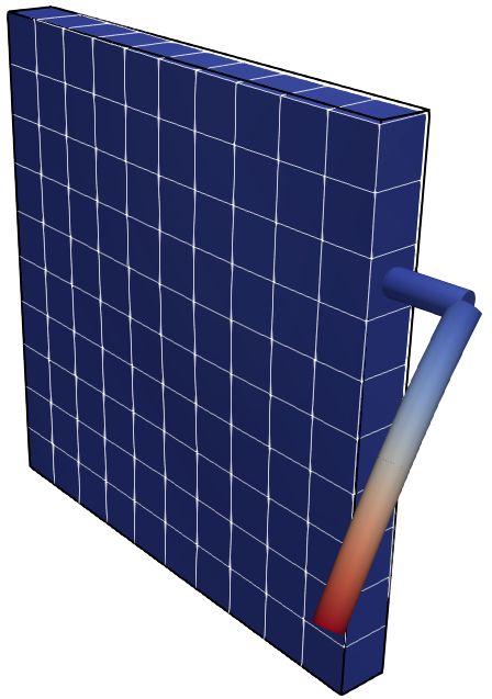
8                                                                                                               Ivo Steinbrecher et al.

                                                                                                       T
4.3.2 Lagrange multiplier potential                                where the identity rv(R∗ ΛR∗ ) = R∗ rv(Λ) has been
                                                                   used. Thus, the rotational coupling conditions (19) in com-
Alternatively, the Lagrange multiplier method can be em-           bination with the proposed solid triad definitions and the
ployed to impose the rotational coupling constraints. A La-        employed geometrically exact beam models are objective.
grange multiplier field λθ = λθ (s) ∈ R3 is therefore defined      As shown in [34], in this case also an associated penalty
on the coupling curve Γc . For now, this field is a purely math-   potential of type (21) or an associated Lagrange multiplier
ematical construct in the sense of generalized coupling forces     potential of type (25) is objective.
associated with the coupling conditions (19). The Lagrange             The previous considerations show objectivity of the pro-
multiplier potential for the rotational coupling is                posed (space-continuous) 1D-3D coupling approaches. How-
        Z                                                          ever, in the realm of the finite element method, cf. Section 6, it
Πλθ =       λTθ ψ SB ds .                                   (25)   is important to demonstrate that objectivity is preserved also
         Γc
                                                                   in the discrete problem setting. It is well known that the dis-
Variation of the Lagrange multiplier potential again leads to      cretized deformation gradient, as required for the definition
a constraint contribution to the weak form, i.e.                   of solid triads, is objective as long as standard discretization
         Z                    Z
                                                                   schemes (e.g. via Lagrange polynomials) are applied to the
δΠλθ =        δλT ψ
                θ SB    ds +      λT
                                   θ δo ψ SB ds .       (26)
           Γc                  Γc                                  displacement field of the solid. Also the employed beam finite
         |       {z
                   δWλθ
                         } |         {z
                                    −δWCθ
                                               }                   element formulation based on the geometrically exact beam
                                                                   theory is objective, even though this topic is not trivial and
Therein, δWλθ and δWCθ are the variational form of the             the interested reader is referred to [36, 38]. Therefore, it can
coupling constraints and the virtual work of the generalized       be concluded that the proposed 1D-3D coupling schemes are
coupling forces λθ , respectively. With (9) the virtual work       objective for the space-continuous as well as for the spatially
of the generalized coupling forces becomes                         discretized problem setting.
           Z
−δWCθ =         (δθ S − δθ B )T T T (ψ SB )λθ ds .       (27)      Remark 4.3 Objectivity is the main reason for formulating
              Γc
                                                                   the rotational coupling constraints (19) based on the relative
Since the multiplicative rotation variations δθ B are work-        rotation vector, i.e. ψ SB = 0, cf. [34]. As alternative choice
conjugated to the moment stress resultants of the beam, the        for the rotational coupling constraints the difference between
term −T T (ψ SB )λθ can be interpreted as a distributed cou-       the beam and solid triad rotation vectors, i.e. ψ B − ψ S =
pling moment acting along the beam centerline.                     0, could be considered. However, such coupling constraints
Remark 4.2 For a vanishing relative rotation ψ 21 = 0, as          would result in a non-objective coupling formulation [34].
enforced in the space-continuous problem setting according
to (19), the identity −T T (ψ SB ) = I holds true and the
                                                                   5 Definition of solid triad field
rotational Lagrange multipliers exactly represent the cou-
pling moments along the beam centerline. However, for the          One of the main aspects of the present work is the definition
discretized problem this is only an approximation.                 of a suitable right-handed orthonormal triad field ΛS in the
                                                                   solid, which is required for the coupling constraint (19). This
4.3.3 Objectivity of full beam-to-solid volume coupling            is by no means a straightforward choice, and different triad
                                                                   definitions will lead to different properties of the resulting
As indicated above, the solid triad field depends on the solid
                                                                   numerical coupling scheme. In the following, a brief moti-
deformation gradient F . It can easily be shown, that the
                                                                   vation will be given for the concept of solid triads before
presented solid triad definitions STR-POL, STR-AVG and
                                                                   different solid triad definitions will be proposed.
STR-ORT, in Section 5 are objective with respect to an arbi-
trary rigid body rotation R∗ ∈ SO3 , i.e.
Λ∗S = ΛS (R∗ F ) = R∗ ΛS (F ).                             (28)    5.1 Motivation of the solid triad concept

The geometrically exact beam model employed in this con-           If the embedded beam is considered as a 3D body, a consis-
tribution is also objective [36, 38], i.e.                         tent 2D-3D coupling constraint between the 2D beam surface
Λ∗B = R∗ ΛB .                                              (29)    and the surrounding 3D solid can be formulated as

Equations (28) and (29) inserted into the definition of the        xB − xS = 0 on          Γ2D-3D .                              (31)
relative beam-to-solid rotation vector according to (20) gives
                                                                   Therein, Γ2D-3D is the 2D-3D coupling surface, i.e. the part
the rotated relative rotation vector,
                                                                   of the beam surface that lies withing the solid volume. In
                           T
ψ ∗SB = rv(R∗ ΛS ΛT
                  BR
                     ∗
                       ) = R∗ ψ SB ,                       (30)    the following, let X S,r denote the line of material solid
Consistent coupling of positions and rotations for embedding 1D Cosserat beams into 3D solid volumes                                         9

points that coincide with the beam centerline in the reference          but also alternative solid triad definitions are possible. Ta-
configuration, i.e. X S,r = r 0 . Furthermore, the orthonormal          ble 1 gives an overview of the solid triad variants proposed
triad ΛS,0 = [g S1,0 , g S2,0 , g S3,0 ] shall represent material       in the following.
directions of the solid that coincide with the beam triad in                 All of these solid triad definitions ΛS = [g̃ S1 , g̃ S2 , g̃ S3 ]
the reference configuration according to                                will be a function of the solid deformation gradient F ,
                                                                        i.e. ΛS = ΛS (F ). Moreover, all solid triad definitions will
ΛS,0 = ΛB,0 .                                                  (32)     be constructed in a manner such that the associated orthonor-
                                                                        mal base vectors g̃ S2 and g̃ S3 represent the effective rotation
The corresponding quantities in the deformed configuration
                                                                        of the non-orthonormal directors g S2 and g S3 in an average
are denoted as xS,r and ΛS . Let us now expand the position
                                                                        sense. Thus, it will be required that g̃ S2 and g̃ S3 lie within a
field in the solid as Taylor series around xS,r , i.e.
                                                                        plane defined by the normal vector
xS = xS,r + F ∆X + O(∆X 2 ),                                   (33)
                                                                                g S2 × g S3
where F is the deformation gradient of the solid accord-                n=                    ,                                           (38)
                                                                                g S2 × g S3
ing to (12). The 1D-3D coupling strategy underlying the
proposed BTS-FULL scheme relies on the basic assump-
tion of slender beams, i.e. R  L, where R is a charac-                 in the following denoted as the n-plane. Eventually, in the
teristic cross-section dimension (e.g. the radius of circular           examples in Section 7, two desirable properties of the solid
cross-sections). This assumption allows to truncate the Tay-            triad field for the proposed BTS-FULL method are identified:
lor series after the linear term as long as small increments
∆X = αg S2,0 + βg S3,0 , with α, β ≤ R, are considered:                 (i) The solid triad should be invariant, i.e. symmetric/unbiased
                                                                             with respect to the reference in-plane beam cross-section
xS ≈ xS,r + αg S2 + βg S3 ,                                    (34)          basis vectors g B2,0 and g B3,0 .
                                                                        (ii) The resulting BTS-FULL method should not lead to
which results in an error of order O(R2 ). Here, the directors               locking effects in the spatially discretized coupled prob-
g S2 and g S3 , which are not orthonormal in general, represent              lem.
the push-forward of the solid directions g S2,0 and g S3,0 :
                                                                        These properties will be investigated for the following solid
g Si := F g Si,0     for i = 2, 3.                             (35)     triad definitions.

It follows from (34) and (15) that the 2D-3D coupling condi-
tions (31) between the beam surface and the expanded solid
position field are exactly fulfilled if the following 1D-3D             5.2 Polar decomposition of the deformation gradient
coupling constraints are satisfied:                                     (STR-POL)

xS,r = r,                                                      (36)     Based on polar decomposition, the deformation gradient of
g S2 = g B2 ,      g S3 = g B3 .                               (37)     the solid problem can be split into a product F = vRS =
                                                                        RS U consisting of a rotation tensor RS ∈ SO3 and a (spa-
Coupling constraints of the form (37) enforce that the mate-            tial or material) positive definite symmetric tensor v or U ,
rial fibers g S2 and g S3 of the solid remain orthonormal dur-          respectively, which describes the stretch. An explicit calcu-
ing deformation, thus enforcing vanishing in-plane strains              lation rule for the rotation tensor, e.g. based on v, can be
of the solid at the coupling point xS,r = r. In Section 7,              stated as:
it will be demonstrated that constraints of this type lead to
severe locking effects when applied to finite element dis-
                                                                         v2 = F F T ,                                                     (39)
cretizations that are relevant for the proposed BTS-FULL                          −1
scheme, i.e. solid mesh sizes that are larger than the beam             RS = v         F.                                                 (40)
cross-section dimensions. It will be demonstrated that such
locking effects can be avoided if the solid triad field is defined      As mentioned above, it is desirable that the orthonormal
in a manner that only captures the purely rotational contri-            base vectors g̃ S2 and g̃ S3 of the solid triad ΛS lie in a plane
butions to the local solid deformation at xS,r = r without              with normal vector n according to (38). It can easily be
additionally constraining the solid directors in the deformed           verified that the rotation tensor RS associated with the total
configuration. As will be demonstrated in the next sections,            deformation gradient F according to (40) will in general
the rotation tensor defined by the polar decomposition of the           not satisfy this requirement. Thus, a modification will be
deformation gradient is an obvious choice for this purpose,             presented in the following to preserve this property.
10                                                                                                                          Ivo Steinbrecher et al.

Table 1 Listing of the different solid triad variants presented in this contribution.

                              solid triad     description
                              STR-POL         obtained from the polar decomposition of the solid deformation gradient
                              STR-DIR2/3      fix one chosen solid material direction to the solid triad
                              STR-AVG         fix average of two solid material directions to the solid triad
                              STR-ORT         orthogonal solid material directions stay orthogonal

5.2.1 Construction of STR-POL triad                                           ḡ 1 = n, ḡ 2 = g S2 /kg S2 k and ḡ 3 = n × ḡ 2 , which coincides
                                                                              with the solid triad definition later discussed in Section 5.3.1.
Since the sought-after solid triad shall be uniquely defined
                                                                                                                             n
already by the two in-plane directors g S2 and g S3 , a modified              Remark 5.1 It can be verified that RS = R2DS R is fulfilled
version of the deformation gradient will be considered,                       for quasi-2D deformation states, e.g. for pure torsion load
                                                                              cases where the beam axis remains straight during the en-
F n = n ⊗ g S1,0 + g S2 ⊗ g S2,0 + g S3 ⊗ g S3,0 ,                  (41)      tire deformation (see example in Section 7.5). In this case,
                                                                              the (simpler) polar decomposition of the total deformation
which consists of the projection of the total deformation
                                                                              gradient F according to (40) can exploited.
gradient F into the n-plane extended by the additional term
n ⊗ g S1,0 . This modified deformation gradient ensures that
the two relevant in-plane basis vectors are correctly mapped,                 5.2.2 Properties of STR-POL triad
i.e. g S2 = F n g S2,0 and g S3 = F n g S3,0 , while the third
basis vector, which is not relevant for the proposed coupling                 In contrast to alternative solid triad definitions that will be in-
procedure, is mapped onto the normal vector of the n-plane,                   vestigated in the following sections, the definition according
i.e. n = F n g S1,0 . This specific definition of a deformation               to (44), referred to as STR-POL or by the subscript (·)POL ,
                                                                              is not biased by an ad-hoc choice of material directors in
gradient allows for the following multiplicative split:
                                                                              the solid that are coupled to the beam. Instead, the rotation
F n = F 2D Rn ,                                                     (42)      tensor RS describes the rotation of material directions co-
          n
                                                                              inciding with the principle axes of the deformation (i.e. it
where R describes the (pure) rotation from the initial solid                  maps the principle axes from the reference to the spatial con-
triad ΛS,0 onto a (still to be defined) orthonormal intermedi-                figuration), which has two important implications: First, the
ate triad Λ̄ = [ḡ 1 , ḡ 2 , ḡ 3 ], whose base vectors ḡ 2 and ḡ 3 lie    choice of material directions that are coupled depend on the
within the n-plane, and F 2D represents a (quasi-2D) in-plane                 current deformation state and will in general vary in time.
deformation between ḡ 2 and ḡ 3 and the non-orthonormal                     Second, the principle axes represent an orthonormal triad per
base vectors g 2 and g 3 . Now, by applying the polar decom-                  definition, and, thus the coupling to the beam triad will not
position only to the in-plane deformation, i.e.                               impose any constraints on the local in-plane deformation of
                                                                              the solid. Consequently, this solid triad variant fulfills both
F 2D = v 2D R2D
             S ,                                                    (43)
                                                                              requirements (i) and (ii) as stated above.
a solid triad can be defined from the initial triad ΛS,0 as:                      Eventually, a further appealing property of the STR-POL
                                                                              triad shall be highlighted. Let θ0 ∈ [−π, π] represent the ori-
             n
ΛS,POL = R2D
          S R ΛS,0 .                                                (44)      entation of arbitrary in-plane directors in the reference con-
                                                                              figuration defined to coincide for solid and beam according
Once an intermediate triad Λ̄ is defined, the required rotation
                  n                                                           to g S,0 (θ0 ) = g B,0 (θ0 ) = cos (θ0 ) g B2,0 + sin (θ0 ) g B3,0 .
tensors R2D
          S and R can be calculated as follows:
                                                                              Their push-forward is given by g S (θS (θ0 )) = F n g S,0 (θ0 )
1.   Rn = Λ̄ΛT   S,0 ,                                                        for the solid and g B (θB (θ0 )) = RB g B,0 (θ0 ) for the beam,
2.   F 2D = F n (Rn )T ,
                                                                              where the angles θS ∈ [−π, π] and θB ∈ [−π, π] represent
3.   (v 2D )2 = F 2D (F 2D )T ,
                                                                              the corresponding in-plane orientations in the deformed con-
4.   R2D
       S = (v )
                2D −1 2D
                       F .
                                                                              figuration (see Appendix A.1 for a detailed definition). Since
The last remaining question is the definition of the triad                    in-plane shear deformation is permissible for the solid but
Λ̄. It can be shown that the choice of this triad is arbi-                    not for the beam, the orientations θS (θ0 ) and θB (θ0 ) cannot
trary and does not influence the result, since a correspond-                  be identical for all θ0 ∈ [−π, π] and arbitrary deformation
ing in-plane rotation offset would be automatically consid-                   states. However, as demonstrated in Appendix A.1, when
ered/compensated (in the sense of a superposed rigid body                     coupling the beam triad to the STR-POL triad according
rotation) via the rotational part R2D
                                   S of the in-plane polar de-                to (44), the beam directors g B (θB (θ0 ) represent the orien-
composition (43). For example, a simple choice is given by                    tation of the solid directors g S (θS (θ0 ) in an average sense
Consistent coupling of positions and rotations for embedding 1D Cosserat beams into 3D solid volumes 11
such that the following L2 -norm is minimized: relies on the average of the directors g 02 and g 03 , cf. Fig-
ure 3(c):
Zπ
(θS (θ0 ) − θB (θ0 ))2 dθ0 → min. for ΛB = ΛS,POL . (45) g 0S2 + g 0S3
g S,AVG = . (49)
−π g 0S2 + g 0S3
In conclusion, STR-POL is an obvious choice for the solid
With this average vector the solid triad can be constructed
triad with many favorable properties, e.g. it represents the av-
as:
erage orientation of material solid directions in a L2 -optimal
manner. However, it requires the calculation of the square ΛS,AVG = R (−(π/4)n) ΛS,AVG,ref
root of a tensor, and more importantly, for latter variation h i (50)
with ΛS,AVG,ref = n, g S,AVG , n × g S,AVG .
and linearization procedures also the first and second deriva-
tives of the tensor square root with respect to the solid de-
The rotation tensor R (−(π/4)n) in (50) represents a "back-
grees of freedom. This results in considerable computational
rotation" of the constructed reference triad ΛS,AVG,ref by an
costs, since this operation has to be performed at local Gauss
angle of −π/4 to ensure that the resulting solid triad aligns
point level. Therefore, alternative solid triad definitions will
with the beam triad in the reference configuration according
be proposed in the following that can be computed more
to (32). In Section 7, it will be shown numerically that the
efficiently, while still being able to represent global system
variant STR-AVG, similar to the variant STR-POL, fulfills
responses with sufficient accuracy.
both requirements (i) and (ii) stated above.
Remark 5.2 Theoretically, an additive director averaging pro-
5.3 Alternative solid triad definitions cedure such as (49) can result in a singularity if the underlying
vectors are anti-parallel, i.e. g 0S2 = −g 0S3 . However, since
All solid triad variants considered in the following rely on the associated material directors are orthogonal in the ref-
the non-orthonormal solid directors g S2 and g S3 according erence configuration, i.e. g T g = 0, and shear angles
S2,0 S3,0
to (35), their normalized counterparts
smaller than π/2 can be assumed, this singularity will not be
g Si relevant for practical applications.
g 0Si := for i = 2, 3 (46)
g Si
5.3.3 Fixed orthogonal solid material directions
and the corresponding normal vector n according to (38). (STR-ORT)
Based on these definitions, three different variants will be
exemplified in the following. In the last considered solid triad definition, both material
directors g 0S2 and g 0S3 are coupled to the solid triad simul-
taneously. This variant enforces that the directors g 0S2 and
5.3.1 Fixed single solid director (STR-DIR2/3 ) g 0S3 remain orthogonal to each other, and thus it is denoted
as STR-ORT, indicated by a subscript (·)ORT . The STR-ORT
In the first variant, denoted as STR-DIR2/3 , the orientation
variant is realized by applying the rotational coupling con-
of one single solid director, either g 0S2 or g 0S3 , is fixed to the
straints (19) twice, once with ΛS,DIR2 according to (47) and
solid triad, cf. Figure 3(b). The choice which solid material
once with ΛS,DIR3 according to (48).
direction to couple is arbitrary. Therefore, two variants will
Opposed to the other triad definitions in this section, this
be distinguished:
version additionally imposes a constraint on the solid dis-
ΛS,DIR2 = n, g 0S2 , n × g 0S2
(47) placement field by enforcing all shear strain components to
vanish at the coupling point. In Section 7, it will be demon-
ΛS,DIR3 = n, g 0S3 × n, g 0S3 ,
(48) strated that this over-constrained solid triad definition can
lead to severe shear locking effects, i.e. requirement (ii) from
Since the variant STR-DIR2/3 does not fulfill the requirement
Section 5.1 is not satisfied. Thus, also this variant will only
(i) as stated above, it will only be considered for comparison
be considered for comparison reasons in the 2D verification
reasons in the 2D verification examples in Section 7.
examples in Section 7.
5.3.2 Fixed average solid director (STR-AVG)
5.4 Variation of the solid rotation vector
In order to solve this problem, i.e. to define a solid triad that
is symmetric with respect to the base vectors g 02 and g 03 , an In the coupling contributions to the weak form (24) and (26)
alternative variant denoted as STR-AVG is proposed, which the multiplicative rotation vector variation δθ S (spin vector)12 Ivo Steinbrecher et al.
This formulation for the solid spin vector is equivalent to the
e3 g DIR one in (52), but only contains the solid triad basis vectors and
2
e2 their variations. Therefore, this definition of the solid spin
e1 ΛS,DIR2 vector is better suited for solid triads constructed via their
basis vector. Especially in the implementation of the finite
element formulation, it is advantageous to avoid the com-
(a) (b) putation and inversion of the transformation matrix in (52).
Nonetheless, in the remainder of this contribution, the solid
g S,AVG
spin vector as defined in (52) is used to improve readability
of the equations.
ΛS,AVG ΛS,ORT
6 Spatial discretization
(c) (d)
In this work, spatial discretization of the beam, solid and
Fig. 3 Illustration of STR-DIR2 , STR-AVG and STR-ORT solid triad coupling problem will exclusively be based on the finite
definitions for an exemplary 2D problem setting. For simplicity it is
element method. In the following, a subscript (·)h refers
assumed that the beam reference triad aligns with the Cartesian frame
e1 , e2 , e3 , i.e. ΛB,0 = I . (a) Reference configuration, (b) STR-DIR2 , to an interpolated field quantity, superscripts (e) and (f )
(c) STR-AVG and (d) STR-ORT. indicate that the quantity is defined for a solid element e and
a beam element f , respectively. Accordingly, (e, f ) refers
to coupling terms between the solid element e and beam
of a solid rotation vector ψ S arises. The spin vector is work-
element f . The global element count is made up of nel,S
conjugated with the coupling moments, i.e. it is required to
solid finite elements and nel,B beam finite elements.
calculate the virtual work of a moment acting on the solid in a
variationally consistent manner. In contrast to the beam spin
vector δθ B , which represents the multiplicative variation of
primal degrees of freedom in the finite element discretization 6.1 Solid and beam problem
of the geometrically exact Simo–Reissner beam theory and
is discretized directly, no such counterpart exists for the solid For the solid domain an isoparametric finite element ap-
field. Therefore, it is assumed that the solid spin vector can proach is used to interpolate position, displacement and vir-
(e)
be stated as a function of a set of generalized solid degrees tual displacement field within each solid element ΩS,h :
of freedom q (which will later be identified as nodal position
S(e)
= N(e) ξ S , η S , ζ S XS(e)
vectors in the context of a finite element discretization) and Xh (53)
their variations δq. The additive variation of the solid rotation S(e)
= N(e) ξ S , η S , ζ S dS(e)
uh (54)
vector ψ S (q) then reads
S(e)
= N(e) ξ S , η S , ζ S δdS(e) .
δuh (55)
∂ψ S (q)
δψ S = δq. (51)
∂q (e)
Therein, N(e) ∈ R3×ndof is the element shape function ma-
The multiplicative and additive variations are related via (7), trix, which depends on the solid element parameter co-
(e)
which gives the spin vector associated with the solid triad as ordinates ξ S , η S , ζ S ∈ R. Furthermore, XS(e) ∈ Rndof ,
(e) (e)
a function of the generalized solid degrees of freedom: dS(e) ∈ Rndof and δdS(e) ∈ Rndof are the element reference
∂ψ (q) position vector, element displacement vector and element
δθ S = T −1 ψ S (q) S
δq. (52) virtual displacement vector, respectively. Each solid element
∂q (e)
has ndof degrees of freedom.
Remark 5.3 Alternatively, the solid spin vector can be ex-
The beam finite elements used in this work are based
pressed by the variations of the corresponding solid triad
on the Simo–Reissner formulation presented in [35, 38].
basis vectors g Si and their variations δg Si , cf. [36, 38]:
Figure 4. illustrates the degrees of freedom for a single
beam finite element. The beam centerline interpolation is
δθ S = δg T g g + δg T
g g + δg T
g g S3
S2 S3 S1 S3 S1 S2 S1 S2 C 1 -continuous based on third-order Hermite polynomials
∂g ∂g with two centerline nodes per element. Each node for the
S2 S3
= g S1 ⊗ g S3 + g S2 ⊗ g S1
∂q ∂q centerline interpolation has 6 degrees of freedom: 3 for the
∂g (f ) (f )
S1
nodal position r̂ i and 3 for the centerline tangent t̂i at
+ g S3 ⊗ g S2 δq. the node, thus resulting in a total of 12 element degrees of
∂qYou can also read