Corona and XUV emission modelling of the Sun and Sun-like stars
←
→
Page content transcription
If your browser does not render page correctly, please read the page content below
Astronomy & Astrophysics manuscript no. main                                                                                          ©ESO 2021
                                              September 8, 2021

                                              Corona and XUV emission modelling of the Sun and Sun-like stars
                                                                                              Munehito Shoda1 and Shinsuke Takasao2

                                                    1
                                                        National Astronomical Observatory of Japan, National Institutes of Natural Sciences, 2-21-1 Osawa, Mitaka, Tokyo, 181-8588,
                                                        Japan e-mail: munehito.shoda@nao.ac.jp
                                                    2
                                                        Department of Earth and Space Science, Graduate School of Science, Osaka University, Toyonaka, Osaka 560-0043, Japan

                                                    Received month dd, yyyy; accepted month dd, yyyy

                                                                                                                 ABSTRACT
arXiv:2106.08915v2 [astro-ph.SR] 7 Sep 2021

                                                    The X-ray and extreme-ultraviolet (EUV) emissions from the low-mass stars significantly affect the evolution of the planetary at-
                                                    mosphere. However, it is, observationally difficult to constrain the stellar high-energy emission because of the strong interstellar
                                                    extinction of EUV photons. In this study, we simulate the XUV (X-ray+EUV) emission from the Sun-like stars by extending the
                                                    solar coronal heating model that self-consistently solves, with sufficiently high resolution, the surface-to-coronal energy transport,
                                                    turbulent coronal heating, and coronal thermal response by conduction and radiation. The simulations are performed with a range
                                                    of loop lengths and magnetic filling factors at the stellar surface. With the solar parameters, the model reproduces the observed so-
                                                    lar XUV spectrum below the Lyman edge, thus validating its capability of predicting the XUV spectra of other Sun-like stars. The
                                                    model also reproduces the observed nearly-linear relation between the unsigned magnetic flux and the X-ray luminosity. From the
                                                    simulation runs with various loop lengths and filling factors, we also find a scaling relation, namely log LEUV = 9.93 + 0.67 log LX ,
                                                    where LEUV and LX are the luminosity in the EUV (100 Å < λ ≤ 912 Å) and X-ray (5 Å < λ ≤ 100 Å) range, respectively, in cgs. By
                                                    assuming a power–law relation between the Rossby number and the magnetic filling factor, we reproduce the renowned relation be-
                                                    tween the Rossby number and the X-ray luminosity. We also propose an analytical description of the energy injected into the corona,
                                                    which, in combination with the conventional Rosner–Tucker–Vaiana scaling law, semi-analytically explains the simulation results.
                                                    This study refines the concepts of solar and stellar coronal heating and derives a theoretical relation for estimating the hidden stellar
                                                    EUV luminosity from X-ray observations.
                                                    Key words. Sun: corona – Stars: coronae – Ultraviolet: stars – X-rays: stars

                                              1. Introduction                                                             netic field of the star (Pevtsov et al. 2003; Vidotto et al. 2014;
                                                                                                                          Kochukhov et al. 2020), stellar EUV emissions are poorly char-
                                              The Sun has an aura of hot plasma called the corona, which has              acterised because they are difficult to observe. EUV photons suf-
                                              a temperature of a few million Kelvin (Edlén 1943). The image               fer from strong absorption by the interstellar medium (Rumph
                                              of the corona has been captured by the Atmospheric Imaging                  et al. 1994), for which stellar EUV spectra are observable only
                                              Assembly (Lemen et al. 2012) of the NASA’s Solar Dynamics                   for nearby stars in the limited range of wavelength (≤ 360 Å,
                                              Observatory (Pesnell et al. 2012). The corona is not unique to the          Ribas et al. 2005; Johnstone et al. 2021). One thus needs to in-
                                              Sun and has been observed to surround low-mass main-sequence                directly estimate or reconstruct the EUV spectrum of a star from
                                              stars in general (Güdel et al. 1997). Due to its high temperature,          other observables. The proposed reconstruction methods include
                                              the corona is the principal source of stellar XUV (X-ray + EUV:             the inversion of the differential emission measure from UV
                                              extreme ultraviolet) emissions.                                             and/or X-ray observations (Sanz-Forcada et al. 2011; Duvvuri
                                                  Stellar XUV emissions drive the expansion and thermal                   et al. 2021), the empirical correlation between other observable
                                              escape of planetary atmospheres (Vidal-Madjar et al. 2003;                  lines and XUV emission (Linsky et al. 2014; Youngblood et al.
                                              Lecavelier des Etangs et al. 2012; Owen & Wu 2013; Ehren-                   2017; France et al. 2018; Sreejith et al. 2020), and/or a combi-
                                              reich et al. 2015; Airapetian et al. 2017). Therefore, describing           nation of them (Diamond-Lowe et al. 2021). However, the em-
                                              the stellar XUV emission in terms of the stellar fundamental pa-            pirical estimations of stellar EUV emission are based on obser-
                                              rameters (luminosity, mass, radius, etc.) is essential in under-            vations with large uncertainty and a limited number of samples,
                                              standing the evolution of a planet and its habitability. Since stel-        and therefore require further validation from different perspec-
                                              lar XUV emissions decrease over time (Güdel et al. 1997; Ribas              tives.
                                              et al. 2005; Telleschi et al. 2005; Claire et al. 2012; Guinan et al.           To circumvent the intrinsic difficulty of stellar EUV obser-
                                              2016) presumably in response to the stellar spin-down (Kraft                vation, this study uses the solar-stellar connection to theoreti-
                                              1967; Skumanich 1972; Barnes 2003; Irwin & Bouvier 2009;                    cally estimate the stellar XUV emission. The solar-stellar theo-
                                              Matt et al. 2015) caused by magnetised stellar wind (Weber &                retical connection is a natural strategy to predict the stellar prop-
                                              Davis 1967; Kawaler 1988; Shoda et al. 2020), the long-term                 erties. For example, by extending the solar coronal theory, Shi-
                                              evolution of the XUV activity of the host star needs to be de-              bata & Yokoyama (2002) modelled the X-ray characteristics of
                                              scribed as well (Tu et al. 2015; Johnstone et al. 2021).                    the stellar coronae, which was later extended by Takasao et al.
                                                  While the observational characteristics of stellar X-ray emis-          (2020) considering the size distribution of active regions. In this
                                              sions have been established, including their correlations with the          study, by extending the solar atmospheric model, the structure
                                              rotation (Pallavicini et al. 1981; Wright et al. 2011) and mag-             of the upper stellar atmosphere and the XUV emission are pre-
                                                                                                                                                                     Article number, page 1 of 25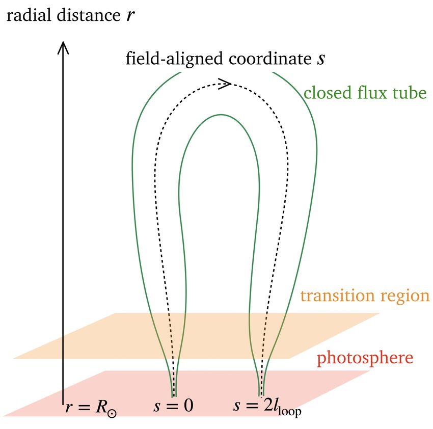
A&A proofs: manuscript no. main

dicted. To this end, the coronal heating problem must be explic-        notation           meaning
itly solved.
     To solve the coronal heating problem, the following three          r                  radial distance from the stellar centre
issues must be addressed (Klimchuk 2006).
1. Energy generation and transfer: the source of the coronal            s                  coordinate along the flux-tube axis
   thermal energy probably comes from the magneto-
                                                                        G                  gravitational constant
   convection on the surface (Steiner et al. 1998). The energy
   generation and transfer to the corona, possibly in the form          kB                 Boltzmann constant
   of Alfvén waves (Alfvén 1947; Osterbrock 1961; Kudoh &
   Shibata 1999; De Pontieu et al. 2007; McIntosh et al. 2011;          mH                 hydrogen mass
   Srivastava et al. 2017), needs to be solved.
2. Energy dissipation in the corona: the magnetic (and kinetic)         me                 electron mass
   energy in the corona needs to dissipate to sustain the
   high-temperature corona. The field-braiding process must be          h                  Planck constant
   considered as a promising mechanism of magnetic-energy
   dissipation (Parker 1972, 1988).                                     M                  solar mass
3. Thermal response to the heating: the density and temper-             R                  solar radius
   ature of a coronal loop are determined by the energy bal-
   ance among heating, conduction and radiation. The Rosner-            T                  solar effective temperature
   Tucker-Vaiana (RTV) scaling law (Rosner et al. 1978) origi-
   nates from the thermal response to coronal heating. Thus, the        Ω                  solar angular rotation rate
   RTV scaling law or its generalised form (Serio et al. 1981;
   Zhuleku et al. 2020) should be reproduced by the model (An-       Table 1. Notations of the coordinates (r and s) and constant parameters.
   tolin & Shibata 2010).                                            Note that subscript denotes the solar fundamental parameter.
For these issues, a model of the coronal heating should 1. in-
clude the photosphere (stellar surface) and chromosphere, 2.
appropriately consider the field-braiding process in the corona,     XUV emission that includes a significant contribution from the
and 3. implement the thermal conduction and radiative cooling.       transition region.
Classically, numerical models of a corona have often focused              Considering the difficulty of the TR problem, we perform
on the thermal responses to heating events by one-dimensional        a series of 1D, high-resolution magnetohydrodynamic (MHD)
(1D) (expanding) flux-tube models (Antiochos & Sturrock 1978;        simulations for a wide range of parameters. This 1D model fa-
Peres et al. 1982; Antiochos et al. 1999). A zero-dimensional        cilitates a coronal loop simulation with sufficiently high numeri-
model of the coronal thermal evolution is also proposed (Klim-       cal resolution. The field-braiding process (or turbulence), which
chuk et al. 2008). The advancement of numerical techniques and       is essentially 3D, must be appropriately modelled when solving
increase in computational power have made models highly so-          the coronal heating problem by 1D simulation. In this study, an
phisticated. Several models deal with the realistic energy gen-      approximated formulation of turbulent dissipation, developed in
eration by explicitly solving the magneto-convection (Hansteen       previous studies (Dmitruk et al. 2002; Shoda et al. 2018), is em-
et al. 2015; Rempel 2017). Other models have focused more            ployed as it is likely to reproduce the average heating rate of the
on energy dissipation with simpler numerical settings (Moriyasu      coronal loop (van Ballegooijen et al. 2011). For simplicity, we
et al. 2004; Rappazzo et al. 2008; van Ballegooijen et al. 2011;     focus on the Sun-like stars that exhibit solar mass, luminosity,
Dahlburg et al. 2016). These models have predicted that the          radius, and metallicity.
signature of coronal heating could be explained by convection-            The rest of the manuscript is structured as follows. In Sec-
driven energy injection. By extending these studies, we aimed        tion 2, the coronal model and numerical methods are detailed.
to construct a stellar coronal model that would satisfy the three    Section 3 produces the numerical results, focusing on the depen-
requirements.                                                        dencies of coronal properties on the loop length and magnetic
    In deriving the X-ray and EUV spectra from simulations,          filling factor that are likely to vary with the star (Reale & Micela
care needs to be taken in the spatial resolution at the transition   1998; Reale et al. 2004; Reiners et al. 2009; See et al. 2019). The
region (the temperature-jump region between the chromosphere         XUV spectra obtained from the simulations are also presented.
and the corona). The numerical resolution around the transition      In Section 4, analytical arguments on the energy flux injected
region is found to significantly affect the coronal density (Brad-   into the corona are presented. In Section 5, the interpretations
shaw & Cargill 2013), and the coronal emission measure dis-          and limitations of the proposed model are discussed. Section 6
tribution (EMD). Because the coronal emission is proportional        summarises the study. Several details are provided in the Ap-
to the EMD, it means that the XUV emission predicted by sim-         pendix, including the resolution dependence of the model (see
ulation significantly depends on the numerical resolution. The       Appendix B).
required resolution is in the order of km or less, which is im-
practical in realistic three-dimensional (3D) simulations. A pre-
vious study attempted to solve this “transition-region problem”      2. Model
by introducing the artificial broadening of the transition region    2.1. Model overview and notation
by tuning the magnitude of radiative cooling and thermal con-
duction (Johnston et al. 2017; Johnston & Bradshaw 2019; Iijima      As mentioned earlier, the aim of this study is to model the XUV
& Imada 2021; Johnston et al. 2021). However, this treatment         (X-ray+EUV) emissions from the Sun and Sun-like stars (in-
may yield an unrealistic EMD in the transition-region temper-        cluding young Sun) with a range of magnetic activity level. To
ature, and therefore is inappropriate for the calculation of the     this end, the luminosity, mass, radius, and metallicity of the stars
Article number, page 2 of 25
Munehito Shoda and Shinsuke Takasao : Corona and XUV emission modelling of the Sun and Sun-like stars
2010), solar and stellar coronal heating (Moriyasu et al. 2004;
Washinoue & Suzuki 2019), and solar wind acceleration (Suzuki
& Inutsuka 2005; Shoda et al. 2018).
Hereinafter, the two perpendicular directions shall be de-
noted by x and y. Thus, the local xy plane is perpendicular to the
axis of the loop. The flux-tube expansion is incorporated through
the scale factors in the x and y directions: h x,y . For simplicity,
the loop is assumed to expand isotropically in the perpendicular
directions. In terms of scale factors, the isotropic expansion is
represented by
h x = hy ∝ A(s),
p
(2)
where A(s) is the cross section of the coronal loop. As h s = 1 by
definition, Eq. (2) results in
1 ∂
∇·X = (X s A(s)) ,
A(s) ∂s
1 ∂ p
∇×X = √ X x A(s) ey (3)
A(s) ∂s
1 ∂ p
− √ Xy A(s) e x
A(s) ∂s
Fig. 1. A schematic picture of the system. One-dimensional dynamics
along the axis of the closed flux tube is simulated. The axis is indicated for any vector field X, where e x,y represent the unit vectors in
by the dotted line, while the flux tube surface is denoted by green lines. the x, y directions. The 1D spherical coordinate system is repro-
The flux tube is intended to be nearly vertical and super-radially ex- duced as a special case of A(s) = s2 .
panding. The geometry of the loop is defined by the filling factor f and The flux tube expands in the chromosphere as a response to
radial distance r as functions of field-aligned distance s.
the exponential decrease in the ambient gas pressure (Cranmer
& van Ballegooijen 2005; Ishikawa et al. 2021). As a result of
are fixed to the solar value, i.e., this expansion, the filling factor of the magnetic field (flux tube)
f should increase nearly exponentially with altitude. Under this
L=L , M=M , R=R , Z=Z . (1) assumption, we model the filling factor f as
" !#
Dependence on metallicity is considered in the radiative loss r−R
f = min 1, f∗ exp , Hmag = cmag H∗ , (4)
function (Section 2.5) and spectrum calculation (Section 3.1). Hmag
We study the dependence of coronal properties on the coronal
loop length and the filling factor of magnetic fields. Because the where f∗ is the magnetic filling factor on the photosphere and
filling factor tends to increase with the stellar rotation rate (or
the Rossby number, Saar 2001; Reiners et al. 2009), the coronal kB T R2
H∗ = (5)
dependence on the stellar rotation rate is implicitly investigated. GM mH
We model a single coronal loop rooted in the stellar surface,
is the pressure scale height at the photosphere. By this formula-
and self-consistently solve the energetics and dynamics inside
tion, we assume that the loop expands only in the chromosphere
the loop. In other words, we solve the time-dependent, 1D MHD
and exhibits a uniform cross section in the corona, which is sup-
equations for an expanding coronal loop. The differential emis-
ported by some solar observations (Klimchuk et al. 1992, but
sion measure (DEM) of a single coronal loop is directly obtained
see a recent discussion by Malanushenko et al. (2021)). Given
from the simulation, which is then converted to the XUV spec-
that the pressure scale height is uniform from the photosphere
trum by prescribing the chemical composition and integrating
up to the chromosphere, cmag = 2 yields a flux-tube expansion
the continuum and line emissions as a function of wavelength
with a constant plasma beta in altitude. In this work, we set
using the CHIANTI atomic database version 10.0 (Dere et al.
cmag = 2.5 that realizes a slightly low-beta chromosphere. We
1997; Del Zanna et al. 2021).
have confirmed that the choice of cmag does not have a signifi-
Notations of the coordinates and constant parameters used in cant influence over the simulation results.
this study are listed in Table 1. X denotes the solar value and X∗
the value of X measured at the photosphere. When the coronal loop extends to a region far above the sur-
face, the flux tube also undergoes the radial expansion ∝ r2 ,
where r is the radial distance from the stellar centre. Consid-
2.2. Model of the closed flux tube ering the chromospheric and radial expansions, the cross section
A is expressed as
A single coronal loop is modelled by a 1D expanding flux tube
rooted in the photosphere. Figure 1 illustrates a schematic of the A ∝ r2 f. (6)
model. As shown in Table 1, the coordinate along the axis of
the flux tube is denoted by s. The spatial variation only along We define the inclination of the flux tube by prescribing r as
the loop is assumed to be nonzero, that is, ∂/∂s , 0. Similar 1D a function of s. We consider nearly vertical flux tubes, so that
flux tube models were used in the models of solar spicules (Holl- the vertical line of sight is nearly aligned with the axis of the
weg et al. 1982; Kudoh & Shibata 1999; Matsumoto & Shibata flux tube (Figure 1). It is easier to calculate the DEM along the
Article number, page 3 of 25A&A proofs: manuscript no. main
1.0 eint denotes the internal energy per unit volume and is defined in
Section 2.4. The source term S is given by
0
0.8
!
1 2 GM dr
p + ρv⊥ /L − ρ 2
2 r ds
1 Bs Bx
0.6 −ρv s v x + + ρD v
x
z/lloop
2L 4π !
1 Bs By
S = 2L
−ρv v
s y + + ρD v
y ,
(12)
4π
0.4
1
(v s Bx − v x Bs ) + 4πρDbx
p
2L
1 p
v s By − vy Bs + 4πρDy b
0.2 2L
GM∗ dr
+ Qcnd + Qrad
−ρv s 2
r ds
0.0
0.0 0.2 0.4 0.6 0.8 1.0 where L−1 = d/ds ln r2 f denotes the length scale of the flux-
tube expansion. The conduction term Qcnd is defined in terms of
x/lloop conductive flux qcnd as
1 ∂
Fig. 2. Shape of the flux-tube axis defined by Eq. (7). x and z denote Qcnd = − q cnd r 2
f . (13)
the horizontal and vertical coordinates, repectively. r2 f ∂s
Because the mean free path of an electron is generally smaller
than the system size, the Spitzer–Härm flux (Spitzer & Härm
1953) is applied to qcnd :
vertical line of sight for this structure. In particular, we set
|Bs | ∂T
qcnd = − κSH T 5/2 , (14)
dr 10 lloop − s |B| ∂s
= tanh , r| s=0 = R (7)
ds lloop where κSH = 10−6 erg cm−1 s−1 K−7/2 . The radiative cooling Qrad
where lloop is the half-loop length. The actual shape of the flux- and turbulent dissipation Dv,bx,y are described in Section 2.5 and
tube axis is displayed in Figure 2. Combining Eq.s (4)–(7), the 2.6, respectively. Because turbulence is considered not as an ex-
cross section A(s) is well defined as a function of s. ternal force but as a dissipative process, the losses of the kinetic
and magnetic energies by turbulence are locally balanced by the
gain in the internal energy. Thus, the presence of the turbulence
terms does not affect the conservation of the total energy. For the
2.3. Basic equations same reason, we do not explicitly consider the numerical dissi-
pation of velocity and magnetic field in the energy equation. We
The MHD equations with the equation of state of partially note that the numerical dissipation is unlikely to be the dominant
ionised hydrogen, gravity, thermal conduction, radiative cooling, heating mechanism because the coronal Alfvén wave, which has
and phenomenology of turbulent heating are selected as the ba- a typical wavelength of ∼ 100 Mm, is resolved by a sufficiently
sic equations of the model, which are expressed in the form of fine grid in the corona (100 km).
conservation law (for derivation, see Appendix A)
∂ 1 ∂ 2 2.4. Equation of state
U+ 2 Fr f = S. (8)
∂t r f ∂s We assume that the plasma consists of neutral hydrogen atoms,
protons, and electrons. The internal energy per unit volume eint
The conserved variables U and the corresponding fluxes F are
is composed of the conventional thermal energy p/(γ − 1) and
given by
the latent heat of the ionised gas.
ρ ρv s
p
eint = + nH χIH , nH = ρ/mH ,
ρv s ρv s + pT
2 (15)
γ−1
ρv x ρv s v x − Bs Bx /(4π)
U = ρvy , F = ρv s vy − Bs By /(4π) , (9) where χ is the ionisation degree and nH is the number density of
hydrogen atoms (proton + neutral hydrogen). IH is the ionisation
Bx
v B
s x − v B
x s
energy of the hydrogen atom (IH = 13.6 eV). We assume that the
By v s By − vy Bs
e (e + pT ) v s − Bs (v⊥ · B⊥ ) /(4π) ionisation degree could be determined from the approximated
version of the Saha-Boltzmann equation, in which only the
where ground state is considered as the bound state (low-temperature
limit).
v⊥ = v x e x + vy ey , B⊥ = Bx e x + By ey , (10)
χ2
!
B2⊥ 1 B2⊥ 2 IH
pT = p + , e = eint + ρv2 + . (11) = exp − , (16)
8π 2 8π 1 − χ nH λ3e kB T
Article number, page 4 of 25Munehito Shoda and Shinsuke Takasao : Corona and XUV emission modelling of the Sun and Sun-like stars
radiative loss function [erg cm3 s−1] 10−21 mosphere exhibits isothermal behaviour in the absence of other
cooling/heating mechanisms.
The optically thin cooling is expressed in terms of the radia-
10−22 tive loss function Λ(T ) by ne nH Λ(T ). In this work, we define the
loss function over a wide range of temperature (103 K ≤ T ≤
107 K) as follows.
10−23
1. For simplicity, in the high-temperature range (T ≥ 1.5 ×
104 K), the cooling rate is referred from the CHIANTI
10−24 atomic database with the photospheric abundance (no first
ionisation potential (FIP) effect).
CHINATI loss function 2. The cooling rate in the low-temperature range (T ≤ 1.0 ×
10−25 Λeff (T ) 104 K) is deduced by Goodman & Judge (2012), which par-
Λ(T ) tially consider the non-LTE effect.
10−26 3. In the intermediate-temperature range (1.0 × 10⁴ K < T <
104 105 106 107 1.5 × 10⁴ K), a bridging law between two loss functions asre
T [K] employed following the method of Iijima (2016).
Fig. 3. Solid and dashed lines show the effective and original optically- The chromospheric heating effect by backward coronal radiation
thin radiative loss functions Λeff (T ) and Λ(T ), respectively. Also shown is still missing in Λ(T ) defined above. To introduce this effect,
by crosses are the loss function from the CHIANTI atomic database we quench Λ(T ) in the chromospheric temperature range, which
with photospheric abundance. gives Qthin
rad
2
T
where λe is the thermal de Broglie wavelength of electron. Qrad = ne nH Λeff (T ), Λeff (T ) = Λ(T ) exp − chr
thin , (22)
T2
s
h2 where T chr = 2.0 × 10⁴ K. The effective radiative loss function
λe = . (17) Λeff (T ) is displayed in Figure 3, along with the original radiative
2πme kB T
loss function Λ(T ) and the CHIANTI loss function defined in
When chromospheric hydrogen is no longer in thermal equi- T ≥ 104 K.
librium, the ionisation degree will deviate from the Saha–
Boltzmann value (Goodman & Judge 2012), which is beyond
2.6. Phenomenological model of coronal turbulence
the scope of this study. Once the ionisation degree χ is obtained,
the pressure and temperature are related by Although the mechanism of the coronal heating is debated, it
is of no doubt that magnetic field feeds heat to the corona that
p = (ne + nH ) kB T = (1 + χ) nH kB T. (18) maintains the million-Kelvin temperature by dissipation. The
formation of tangential discontinuities (electric current sheets) in
2.5. Radiation response to the continuous shuffling of the foot points of coro-
nal magnetic fields is a plausible mechanism of magnetic-field
The radiative cooling rate per unit volume Qrad is given by dissipation (Parker 1972; Sturrock & Uchida 1981; Parker 1983;
van Ballegooijen 1986; Galsgaard & Nordlund 1996). The ubiq-
Qrad = ξrad Qthck
rad + (1 − ξrad ) Qrad ,
thin
(19) uitous current-sheet formation should lead to small-scale impul-
p
! sive energy release, which is likely to feed a sufficient amount
ξrad = 1 − exp − , prad /p∗ = 0.1, (20) of energy to the corona, possibly in the form of micro- and
prad nano-flares (Parker 1988; Shimizu 1995; Aschwanden & Parnell
2002).
where p∗ is the pressure at the surface (photosphere) and Qthck rad The formation of current sheets can be interpreted as turbu-
and Qthin
rad approximate the optically thick and thin cooling rates, lent cascading (Rappazzo et al. 2007, 2008; Verdini et al. 2012).
respectively. The optically thick and thin functions are seam- Because the coronal loop is threaded by a strong mean mag-
lessly connected via ξrad . Instead of solving the radiative transfer, netic field, the MHD turbulence evolving in the coronal loop can
we model Qthck thin
rad and Qrad as follows. be accurately approximated by the reduced-MHD turbulence,
The radiative heating and cooling are approximately bal- in which the energy cascades preferentially in the perpendicu-
anced near the photosphere to maintain a nearly constant sur- lar direction (Shebalin et al. 1983; Cho & Vishniac 2000; Cho
face temperature. The optically thick radiative loss is approxi- & Lazarian 2003). The energy-cascading (or heating) rate of
mated by an exponential cooling function that forces the local the reduced-MHD turbulence, Qheat , is precisely approximated
temperature to approach the reference value (Gudiksen & Nord- by the mean-field quantities as follows (Hossain et al. 1995;
lund 2005): Matthaeus et al. 1999; Dmitruk et al. 2002; Verdini & Velli 2007)
!−1/2
1 ref ρ z+⊥ z−⊥ 2 + z−⊥ z+⊥ 2
Qrad =
thck
e − eint , τ = 0.1 s , (21) Qheat ≈ cd ρ , (23)
τ int ρ∗ 4λ⊥
where ρ∗ is the photospheric mass density and erefint is the refer- where z±⊥ denotes the (root-mean-squared (RMS)) amplitude of
ence internal energy density corresponding to the reference tem- the perpendicular Elsässer variables and λ⊥ is the correlation
perature T ref . We simply assume T ref = T , i.e., the stellar at- length of the Elsässer variable (Alfvén wave) perpendicular to
Article number, page 5 of 25A&A proofs: manuscript no. main
the mean field. cd is a dimensionless parameter. By this approx- The photospheric magnetic field is known to form localised kilo-
imation, we estimate the averaged heating rate using the coronal Gauss patches (Spruit & Zweibel 1979; Tsuneta et al. 2008).
turbulence (field braiding). These patches are likely to be in thermal equipartition, which
The approximated heating rate in Eq. (23) is implemented by equates the gas and magnetic pressures. For the non-magnetised
adding the source terms Dvx,y , Dbx,y given by Shoda et al. (2018). photosphere, the thermal equipartition field is given by
cd Beq = 1.34 × 10³ G. (33)
z+x,y z−x,y + z−x,y z+x,y ,
Dvx,y = − (24)
4λ⊥ In the magnetised photosphere, as the deeper region tends to
cd
z+x,y z−x,y − z−x,y z+x,y ,
Dbx,y =− (25) be observed (e.g. Keller et al. 2004), the ambient gas is likely
4λ⊥ to exhibit larger pressure than the non-magnetised photosphere.
Thus, the equipartition magnetic field should be larger than this
where z±x,y = v x,y ∓ Bx,y / 4πρ. The role of these terms is ex-
p
equipartition value. Therefore, we set the photospheric axial
plained below. Without the conservation part ∝ ∂ r2 f F /∂s, the magnetic field equal to
perpendicular components of the equation of motion and induc-
tion equation are expressed as Bs,∗ = 1.5Beq = 2.01 × 10³ G. (34)
∂ ∂
ρv x,y = ρDvx,y , Bx,y = 4πρDbx,y ,
p
(26)
∂t ∂t We model the energy injection from the photosphere by im-
In the limit of the reduced-MHD approximation (time- posing the velocity and magnetic-field fluctuations. Fluctuations
independent density, ∂ρ/∂t = 0), Eqs. (24), (25), and (26) are are imposed at both ends of the simulation domain. The verti-
reduced to cal and horizontal velocity fluctuations are modelled separately.
The upward acoustic waves are excited on the photosphere by
∂ ± cd ∓ ± employing the time-dependent boundary conditions on the den-
z =− z z , (27)
∂t x,y 2λ⊥ x,y x,y sity and axial velocity.
!
which yields the energy conservation law of v s,∗
ρ∗ = ρ∗ 1 + , (35)
X z− z+ 2 + z+ z− 2 a∗
∂ i i i i
e⊥ = −cd ρ , (28) Z ωlmax
∂t
h i
i=x,y
4λ⊥ v s,∗ = dω ṽ s (ω) sin ωt + ψl (ω) , (36)
ωlmin
where e⊥ is the sum of the kinetic and magnetic energies emerg-
ing from the fluctuations of the perpendicular components: where ρ∗ is the time-averaged photospheric density, a∗ =
√
kB T ∗ /mH is the isothermal speed of sound on the photosphere,
1 +2 2
1 B2 and ψl (ω) is a random phase function that ranges between 0 and
e⊥ = ρ z⊥ + z−⊥ = ρv2⊥ + ⊥ . (29) 2π. In the numerical implementation of the integral in Eq. (36),
4 2 8π
the frequency range is evenly divided into 21 bins and the corre-
Comparing Eq.s (23) and (28), one obtain sponding 21 components are summed. The time-averaged pho-
tospheric density is given by equipartition on the photosphere:
∂
e⊥ ≈ −Qheat , (30)
∂t B2s,∗
ρ∗ kB T ∗ /mH = , (37)
indicating that the energy dissipation by the reduced-MHD tur- 8π
bulence is considered appropriately. which yields
The perpendicular correlation length is assumed to increase
with the flux-tube radius, i.e., ρ∗ = 4.22 × 10⁻⁷ g cm−3 . (38)
ρ∗ is larger than the typical mass density on the solar surface be-
r s
A r f
λ⊥ = λ⊥,∗ = λ⊥,∗ , (31) cause the magnetised photosphere should be deeper and denser.
A∗ R f∗ The (time-averaged) Alfvén speed vA on the photosphere is then
expressed as
where the perpendicular correlation length at the photosphere is
set equal to the typical width of the inter-granular lane: λ⊥,∗ = Bs,∗
150 km. However, the best possible free parameter cd is still de- vA,∗ ≈ p = 8.73 km s−1 . (39)
4πρ∗
bated. In this study, we infer cd = 0.1 from the previous studies
of the solar-wind turbulence (van Ballegooijen & Asgari-Targhi We arbitrarily set ṽ s (ω) ∝ ω−1/2 with
2017; Chandran & Perez 2019; Verdini et al. 2019).
2π/ωlmin = 300 s, 2π/ωlmax = 100 s. (40)
2.7. Boundary condition and simulation setting The minimum frequency corresponds to the cut-off frequency of
the acoustic wave at the photosphere (e.g. Felipe et al. 2018).
Both boundaries of the simulation domain are located at the pho- The magnitude of ṽ s (ω) is tuned such that the RMS amplitude
tosphere, and the photospheric temperature is fixed to the effec- of v s,∗ at the photosphere is 0.6 km s−1 .
tive temperature, i.e.,
q
T ∗ = T = 5.77 × 10³ K. (32) v2s,∗ = 0.6 km s−1 , (41)
Article number, page 6 of 25Munehito Shoda and Shinsuke Takasao : Corona and XUV emission modelling of the Sun and Sun-like stars
where the overline denotes the time average. Although the magnetic filling factor half-loop length
longitudinal-wave excitation on the photosphere is explicitly (photosphere) [103 km]
considered, the effect of the longitudinal-wave input is insignif-
icant; the coronal temperature decreases by only 2% when the f∗ = 1 lloop = [20, 30, 40]
longitudinal wave injection is terminated.
f∗ = 0.5 lloop = [20, 30, 40]
The horizontal velocity and magnetic field at the bottom
boundary are expressed in terms of the Elsässer variables, which f∗ = 0.333 lloop = [20, 30, 40, 60]
are defined as
f∗ = 0.2 lloop = [20, 30, 40]
Bx,y
z±x,y = v x,y ∓ p . (42)
4πρ f∗ = 0.1 lloop = [20, 30, 40, 60, 80]
The free boundary condition is imposed on the downward El- f∗ = 0.05 lloop = [20, 30, 40]
sässer variables.
lloop = [20, 30, 40, 60,
∂ − f∗ = 0.0333
z = 0. (43) 80, 120, 160, 240]
∂s x,y ∗
lloop = [20, 30, 40, 60, 80, 120,
The upward Elsässer variable is assumed to be non- f∗ = 0.01 = f
160, 240, 320, 480, 640]
monochromatic with respect to the frequency.
Z ωtmax f∗ = 0.005 lloop = [20]
+
h i
z x,y,∗ = dω z̃±x,y (ω) sin ωt + ψt (ω) , (44)
ωtmin Table 2. List of the simulation runs conducted in this study. The mag-
netic filling factor on the solar photosphere is set to f = 0.01 (Cranmer
where ψt (ω) is a random phase function that ranges between 0 2017).
and 2π. As with Eq. (36), the frequency range is discretised into
21 bins when numerically implementing the integral in Eq. (44).
We set z̃±x,y (ω) ∝ ω−1/2 with
it reaches the maximum ∆smax . In particular, in 0 ≤ s ≤ lloop , the
2π/ωtmin = 1000 s, 2π/ωtmax = 100 s. (45) size of the i-th cell, ∆si , is iteratively defined as
z̃±x,y (ω) ∝ ω−1/2 corresponds to the 1/ω energy spectrum dis-
" " ##
2εge
∆si = max ∆smin , min ∆smax , ∆smin + si−1 − sge ,
covered in previous solar simulations and observations (Van 2 + εge
Kooten & Cranmer 2017). Given that the typical size of a gran- 1
ule is 1, 000 km and the typical speed of surface convection is si = si−1 + (∆si−1 + ∆si ) , (48)
1 km s−1 (Chitta et al. 2012), the maximum wave period corre- 2
sponds to the turn-over time of granular motion. Similarly, given Letting N be the total number of cells, we express the cell size
that the typical size of an inter-granular lane is 100 km, the min- in the latter half of the domain lloop ≤ s ≤ 2lloop by
imum wave period corresponds to the turn-over time of inter-
granular motion. The magnitude of z̃±x,y (ω) is tuned such that 1
∆si = ∆sN+1−i , si = si−1 + (∆si−1 + ∆si ) , (49)
the root-mean-squared amplitude of z+x,y,∗ at the photosphere is 2
1.2 km s−1 : The maximum cell size is fixed to ∆smax = 100 km. The relation
q q between the minimum cell size and f∗ is
z+x,∗ 2 = z+y,∗ 2 = 1.2 km s−1 , (46)
∆smin = 5 km ( f∗ < 0.05), ∆smin = 2 km ( f∗ ≥ 0.05). (50)
where the overline denotes the time average. Although some so-
lar observations have observed the suppression of convective ve- This relation is used because a higher resolution is required
locity in large-filling-factor regions (e. g. Katsukawa & Tsuneta at the transition region in the large- f∗ runs (for details, see
2005), we dismiss this effect for simplicity. Appendix B). The grid expansion rate also depends on f∗ as
By this formulation, the energy flux of the upward Alfvén εge = 2.13 ( f∗ < 0.05) and εge = 1.89 ( f∗ ≥ 0.05). The grid
wave at the footpoint of the flux tube is given by expansion height is fixed to sge = 10, 000 km, which is greater
than the typical height of the transition region that needs to be
1 1 resolved with the minimum cell size.
F A,∗ = ρ z2x,∗ + z2y,∗ vA,∗ ≈ ρ∗ z2x,∗ + z2y,∗ vA,∗ In numerically solving Eq. (8), we rewrite the basic equa-
4 4
= 2.65 × 10 erg cm s ,
9 −2 −1
(47) tions in terms of the cross-section-weighted conserved variables
Ũ and the corresponding fluxes F̃ defined by
which is sufficiently larger than the energy flux required to sus- ρ̃ ρr2 f
tain the solar corona (Withbroe & Noyes 1977).
ρ̃ṽr ρvr r2 f
ρ̃ṽ x ρv x r f
2
2.8. Numerical method Ũ = ρ̃ṽy = ρvy rp f , 2
(51)
B̃x B r f
A non-uniform grid system is used to resolve the computational x
B̃y By r p f
domain 0 ≤ s ≤ 2lloop . A uniform cell size of ∆smin is used below
ẽ er2 f
the critical height s < sge , above which the cell size expands until
Article number, page 7 of 25A&A proofs: manuscript no. main
ρ̃ṽr
thermal conduction, which reduce the numerical cost and time
ρ̃ṽ2r
+ p̃T with minimum loss of accuracy.
ρ̃ṽr ṽ x − B̃r B̃x /(4π)
F̃ = ρ̃ṽr ṽy − B̃r B̃y /(4π) ,
(52)
ṽr B̃x − ṽ x B̃r 3. Simulation result
ṽr B̃y −ṽy B̃r
3.1. Fiducial (solar) case: atmosphere and spectrum
(ẽ + p̃T ) ṽr − B̃r ṽ⊥ · B̃⊥ /(4π)
First, we discuss the simulation run with lloop = 20 Mm and
where f∗ = 1.0 × 10⁻² as the fiducial case. In this case, the coronal
2
field strength is ≈ 20 G, which is within the range of the solar
B̃⊥ coronal magnetic field strength measured by the coronal seis-
p̃T = p̃ + = pT r2 f. (53)
8π mology technique (Nakariakov & Ofman 2001; Verwichte et al.
2004; Jess et al. 2016), and thus the fiducial case is regarded as
Using Ũ and F̃, the basic equation is given by the solar case.
∂ ∂ Figure 4 illustrates the time-averaged properties of a quasi-
Ũ + F̃ = S̃, (54) steady coronal loop. Panels show the mass density (top) and tem-
∂t ∂s perature (middle) along the loop axis and the differential emis-
where sion measure (DEM, bottom), defined by
! 0
dllos
DEM(T ) = n2e (T ) , (56)
1 GM∗ dr dT
p̃ + ρ̃ṽ⊥ /L − ρ̃ 2
2
2 !r ds
where ne (T ) is the electron density with temperature T and llos is
1 B̃r B̃x
−ρ̃ṽr ṽ x + + ρ̃Dvx the length along the line of sight. Practically, dividing the tem-
2L 4π ! perature range into bins and considering the vertical line of sight
S̃ = 1 B̃r B̃y . (55) (llos = r), the DEM and associated emission measure distribution
−ρ̃ṽr ṽy + + ρ̃Dvy
(EMD) are numerically obtained as follows
2L 4π
p4πρ̃Dbx
p b
DEM(T i )∆T i ≡ EMD(T i ) = n2e (T i ) ∆r(T i ),
(57)
4πρ̃Dy
GM∗ dr
where ne (T i ) is the total number density of an electron that ex-
−ρ̃ṽr 2 + Qcnd r2 f + Qrad r2 f
r ds hibits a temperature in [T i − ∆T i /2, T i + ∆T i /2] and ∆r(T i ) is the
total radial extension of where T i − ∆T i /2 ≤ T < T i + ∆T i /2.
With this variable conversion, any MHD solver designed for the The DEM is calculated in the temperature range of 104 K ≤ T ≤
Cartesian coordinate system can be directly applied to Eq. (54). 107 K with an equal spacing in the logarithmic scale of T . The
In this study, the Harten–Lax–van Leer discontinuities (HLLD) DEM in the range of T < 104 K is not calculated because, in
approximated Riemann solver (Miyoshi & Kusano 2005) is used the low-temperature range, the atmosphere is not optically thin
to calculate F̃ at the cell boundary. For spatial reconstruction, the and the DEM loses its meaning. Note that the unit of EMD is
fifth-order accurate monotonicity-preserving method (Suresh & cm−5 , while the “volume” EMD, which has often been used in
Huynh 1997) is used to reconstruct the cross-section-weighted the literature (Güdel et al. 2003; Scelsi et al. 2005), represents
conserved variables Ũ in s ≤ sge and 2lloop − s ≤ sge , whereas the the distribution of an emission measure over the whole coronal
monotonic upstream-centred scheme for the law of conservation volume and has a different unit (cm−3 ).
(van Leer 1979) with a minmod flux limiter is used in sge < s <
The high-temperature (T > 106 K) corona is successfully re-
2lloop − sge .
produced in the fiducial case. Since we are imposing the phe-
Thermal conduction and the other parts are solved indepen- nomenological, mean-field formulation of the coronal heating
dently by the second-order operator-splitting procedure as fol- (field braiding/turbulence), the heating tends to be more con-
lows. stant in time and more uniform in space than the actual three-
dimensional case in which the heating is intermittent in time and
1. thermal conduction is solved for a half step ∆t/2: space. Nevertheless, the time-averaged heating rate should be
n ∆t/2 ∗
Ũ −−−→ Ũ (thermal conduction only) similar between the 1D approximation and the 3D simulation,
because the previous 3D simulation of solar wind yielded a simi-
2. the rest of the basic equations are solved for a full step ∆t: lar mean field to the 1D simulation with turbulence phenomenol-
∗ ∆t ∗∗ ogy (Shoda et al. 2019).
Ũi −→ Ũi (without thermal conduction)
Under the assumption that the upper atmosphere (T ≥
104 K) is optically thin in the wavelength of interest, the XUV
3. thermal conduction is solved again for a half step ∆t/2:
∗∗ ∆t/2 n+1
spectrum is obtained from the EMD using the open-source pack-
Ũi −−−→ Ũi (thermal conduction only) age ChiantiPy based on CHIANTI database ver 10.0 (Del Zanna
n
et al. 2021). In particular, the specific intensity Iλ was calcu-
where Ũ is the n-th step value of Ũ. With this procedure, we lated from the EMD using the ChiantiPy.core.Spectrum module
avoid the severe constraints on the ∆t from thermal conduction with the coronal abundance given by Schmelz et al. (2012). Al-
when updating the MHD equations. though the radiative loss function Λ(T ) is constructed with pho-
The third-order strong-stability-preserving (SSP) Runge– tospheric abundance, because the loss function is nearly inde-
Kutta method is used in the time integration of the MHD equa- pendent of the FIP effect in the radiation-dominated temperature
tions (Shu & Osher 1988; Gottlieb et al. 2001). The super-time- range T ≤ 3 × 10⁵ K, the inconsistency in abundance do not vi-
stepping method (Meyer et al. 2012, 2014) is used to solve the olate the simulation results. Assuming that the stellar corona is
Article number, page 8 of 25Munehito Shoda and Shinsuke Takasao : Corona and XUV emission modelling of the Sun and Sun-like stars
10−6 102
flux at 1 au [erg cm−2 s−1 Å−1]
reconstructed from simulated DEM
time average
101 observed solar spectrum (solar minimum)
10−8 snapshot
100
ρ [g cm−3]
10−10 10−1
10−2
10−12
10−3
10−14 10−4
10−16 10−5
0 10 20 30 40 Lyman edge
10−6
s [Mm] 0 200 400 600 800 1000 1200
107
wavelength [Å]
TR TR
Fig. 5. Observed (blue) and simulated (red) spectral flux density of the
106 Sun measured at 1 au. The observed spectrum is retrieved in the solar
activity minimum. The two spectra are in a good agreement below the
Lyman edge (≤ 912 Å).
T [K]
105
& Lightman 1979)
4
10 R 2
Fλ = πIλ , (58)
r
103 which yields the X-ray and EUV luminosities as
0 10 20 30 40 Z 100 Å Z 912 Å
s [Mm] LX = 4πr2 dλ Fλ , LEUV = 4πr2 dλ Fλ . (59)
5Å 100 Å
1029
In terms of energy, X-ray photons are in the range of 0.12 −
2.48 keV. Caution must be exercised when calibrating the X-
1027 rays because a subtle difference in the bandpass of the instrument
DEM [cm−5 K−1]
can result in large differences in the derived response function
and X-ray luminosity (Zhuleku et al. 2020). For the procedure of
1025 translation between different instruments, see Judge et al. (2003).
To test the capability of our model in the prediction of XUV
1023 spectrum, we compare in Figure 5 the spectral flux density ob-
tained from our simulation (red) and that from the observation
in a solar activity minimum (blue). The observed spectrum is
1021 obtained from the coordinated observation in the Whole Helio-
sphere Interval (WHI, from March 20, 2008 to April 16, 2008
1019 Woods et al. 2009; Chamberlin et al. 2009). Figure 5 shows that,
104 105 106 107 below the Lyman edge (≤ 912 Å), the simulated spectrum is in
T [K] a good agreement with the observed spectrum. Above the Ly-
man edge (≥ 912 Å), the continuum is underestimated, and the
emission lines are overestimated in the simulated spectrum, pos-
Fig. 4. Simulated loop properties of the fiducial case. Top: time-
averaged (solid line) and snapshot (dashed line) profiles of mass den-
sibly because the optically thin approximation is inadequate in
sity along the loop axis. Middle: time-averaged (solid line) and snapshot this wavelength range. In this study, because the focus is on the
(dashed line) profiles of temperature along the loop axis. Bottom: time- spectrum below the Lyman edge, the simulation is validated with
averaged differential emission measure (solid line). Annotations “TR” respect to spectrum prediction.
in the middle panel indicate the locations of the transition region in the
snapshot profile.
3.2. Loop-length dependence: Density and temperature
The coronal loop length is a fundamental parameter that affects
the coronal density and temperature. Here, we show the relation
a uniformly bright sphere, the spectral flux density at the helio- between the time-averaged coronal properties and the coronal
centric distance r is deduced by (see, e.g., Section 1.3 of Rybicki loop length. For simplicity, we fix the magnetic filling factor to
Article number, page 9 of 25A&A proofs: manuscript no. main
Ttop [106 K] pbase [dyne cm−2] 101 Another factor that should be considered is the gravitational
stratification. The effective half-loop length often exceeds the
coronal pressure scale height. In such cases, the loop-top pres-
sure in the original RTV scaling law is replaced by the coronal-
base pressure (Serio et al. 1981). Given that the pressure is con-
tinuous across the transition region, we define the coronal-base
pressure pbase as the pressure measured at T ave = 105 K. For
the coronal electron density, both the loop-top value ne,top and
100
coronal-base value ne,base are measured. In contrast to pressure,
the density is discontinuous across the transition region, and
Ttop therefore the definition of the coronal-base density is not triv-
pbase ial. Here, we define ne,base as the value measured in the coronal
eff
∝ lloop
0.39 base:
0.25
Z scor,2
eff
∝ lloop 1
ne,base ≡ ne,ave ds, (61)
10−1 scor,2 − scor,1 scor,1
101 102 103
eff
lloop [Mm] where we set scor,1 = 10 Mm and scor,2 = 15 Mm. The loop-top
density and temperature are given by
1010
ne,top = ne s = lloop , T top = T s = lloop . (62)
ne,top
ne,base eff
Figure 6 shows the lloop -dependencies of the time-averaged
eff −0.49
∝
ne,top ne,base [cm−3]
lloop coronal properties (density, temperature and pressure). The loop-
0.10
eff
∝ lloop top temperature and coronal-base pressure obey a power–law re-
lation with respect to the effective half-loop length, which is for-
mulated as
109
0.39
eff
T top ∝ lloop , (63)
eff 0.25
pbase ∝ lloop . (64)
The (generalised) RTV scaling law predicts that the loop-top
temperature obeys the following relation
108 eff 1/3
101 102 103
RTV
T top ∝ pbase lloop , (65)
eff
lloop [Mm] where we dismiss the exponential correction term as it is negligi-
ble (Serio et al. 1981). A comparison of Eqs. (63), (64), and (65)
eff reveals that the simulation results are consistent with the RTV
Fig. 6. Top: relation between the effective half loop length lloop (see
scaling law.
Eq. (60) for definition) and the time-averaged loop-top temperature
(T top , red circles) and coronal-base pressure (pbase , blue diamonds). Bot- An alternative form of the RTV scaling law predicts a rela-
eff
tom: relation between the effective half loop length lloop eff
and the time- tion among the coronal energy flux Fcor , loop length lloop , and
RTV
averaged loop-top electron density (ne,top , red circles) and coronal-base loop-top temperature T top , and is expressed as
electron density (ne,base , blue diamonds). In both panels, lines represent
the power-law fittings to the symbols. eff 2/7
RTV
T top ∝ Fcor lloop . (66)
A comparison of Eqs. (63) and (66) indicates that the energy flux
the fiducial (solar) value: f∗ = f = 0.01. Hereinafter, the time- injected into the corona is larger for longer loops. In terms of the
averaged value of X will be denoted by Xave . heating rate per unit volume Q, the RTV predictions,
4/7
In the discussion on the behaviour of the coronal properties, RTV
T top ∝ Q2/7 lloop
eff
, (67)
the results must be compared with the analytical RTV scaling
eff 5/7
law (Rosner et al. 1978). Note that the half-loop length in the pRTV
base ∝ Q6/7 lloop , (68)
RTV scaling law denotes the length from the transition region
to the apex of the loop, whereas lloop stands for the length from and simulation results from Eqs. (63) and (64) indicate that
the stellar surface to the apex of the loop. For better comparison, Q = Fcor /lloop
eff eff
is a decreasing function of lloop . These conclu-
eff sions shall be directly validated in the following section.
instead of lloop , we use the effective half-loop length lloop , which
denotes the coronal length, and is defined as The bottom panel of Figure 6 shows the variations in loop-
eff
Z lloop top and coronal-base electron densities over lloop . Given that the
RTV scaling law predicts a larger loop-top density at a higher
eff
lloop = ds, (60)
sTR loop-top temperature for a uniform corona, the decrease in the
loop-top density is attributed to gravitational stratification. Note
where sTR (< lloop ) is where T ave = 105 K. that the coronal-base density exhibits a weaker dependence on
Article number, page 10 of 25Munehito Shoda and Shinsuke Takasao : Corona and XUV emission modelling of the Sun and Sun-like stars
107 ference in the position of the coronal base yields a significant er-
Fcnd measured at Tave = 106 K ror or uncertainty in Fcor . Therefore, instead of directly measur-
Fcnd averaged in [10Mm, 15Mm] ing Fcor , we measure the backward conductive flux Fcnd , which
∝ lloop 0.51 should be balanced with Fcor by energy conservation.
Fcnd [erg cm−2 s−1]
The top and bottom panels in Figure 7 show the loop-length
eff
(lloop and lloop ) dependence of the coronal conductive flux. The
factor 4 difference panels display the simulation runs with a fixed magnetic filling
106 factor of f∗ = 1.00×10⁻² . The red circles and blue diamonds rep-
resent the conductive flux measured at T ave = 1.0×10⁶ K and av-
eraged over 10 Mm ≤ s ≤ 15 Mm, respectively. The black solid
lines represent the power-law fittings to the blue diamonds. The
coronal conductive flux increases with the loop length. How-
ever, the trend deviates from a simple power law. When the
eff
loop length is sufficiently small (lloop . 101.5 Mm) or large
eff
105 (lloop & 102.5 Mm), the conductive flux weakly depends on the
101.0 101.5 102.0 102.5 103.0 eff
loop length. The energy flux increases around lloop ∼ 102.0 Mm,
lloop [Mm] with the minimum and maximum values differing by a factor of
4.
107 An approximate power-law fit to the blue diamonds yields
Fcnd measured at Tave = 106 K the following scaling law
Fcnd averaged in [10Mm, 15Mm]
0.48
eff
∝ lloop
0.48 eff
Fcnd ∝ lloop , (69)
Fcnd [erg cm−2 s−1]
which, in combination with the RTV scaling law, predicts
factor 4 difference
eff 2/7
eff 0.42
106
RTV
T top ∝ Fcor lloop ∝ lloop . (70)
eff
The simulated dependence of T top on lloop , Eq. (63), is repro-
duced by the semi-analytical arguments. Thus, the results shall
be explained semi-analytically once the theoretical behaviour of
Fcor (or equivalently Fcnd ) has been derived. In Section 4, we
propose a simple model to produce Fcor .
105 The enhanced energy injection to the corona produces en-
101.0 101.5 102.0 102.5 103.0 hanced XUV emissions. Figure 8 depicts the loop-length depen-
eff dence of the predicted XUV luminosity. For each coronal loop
lloop [Mm]
calculation, the XUV spectrum is calculated as in Figure 5 and
converted to XUV luminosity through Eq. (59). Both LX and
Fig. 7. Top: half loop length versus coronal conductive flux measured LEUV exhibit increasing trends as those found in the coronal en-
at T ave = 106 K (red circles) and averaged in 10 Mm ≤ s ≤ 15 Mm ergy flux Fcnd . In particular, LX exhibits this trend significantly.
(blue diamonds). Also shown by the solid line is the power-law fitting The inferred power–law relations are
to the blue diamonds. Bottom: same as the top panel but with respect to
eff 0.29
the effective half loop length lloop . eff
LEUV ∝ lloop , (71)
eff 0.65
LX ∝ lloop . (72)
eff
lloop than the coronal-base pressure, which is contradictory if
eff eff
the coronal-base temperature is constant in lloop . It may be in- The dependence of LX on lloop is further explained semi-
eff analytically. The X-ray luminosity should be proportional to the
terpreted that the coronal-base temperature increases with lloop
eff
in response to the increasing T top with lloop . emission measure of the corona, i.e.,
LX ∝ n2cor lloop
eff
, (73)
3.3. Loop-length dependence: Energy flux and XUV where ncor is the typical number density of the coronal loop that
emission lies between nbase and ntop . Assuming that ncor follows the pre-
For a better interpretation of the behaviour of coronal properties, diction of the RTV scaling law,
the variation in the energy flux entering the corona Fcor with the 2 −3/7
eff
effective half-loop length lloop must be revealed.
RTV
ncor ∝ T top /lloop
eff
∝ Fcor 4/7 lloop
eff
, (74)
Directly measuring Fcor from the simulation data is, how- the X-ray luminosity is connected to the coronal energy flux Fcor
ever, not a trivial task. To obtain Fcor , one needs to measure the eff
and loop length lloop by
energy flux at the base of the corona, which moves in time and
is broadened after time averaging. Because a significant amount 1/7 0.69
of energy is reflected back at the transition region, a slight dif- LX ∝ Fcor 8/7 lloop
eff eff
∝ lloop , (75)
Article number, page 11 of 25A&A proofs: manuscript no. main
LX LEUV [erg s−1] 1029 107.0
1028 106.5
Ttop [K]
1027 LX 106.0
LEUV
∝ lloop 0.70 Ttop
∝ lloop 0.31 ∝ f∗0.29
1026
101.0 101.5 102.0 102.5 103.0 105.5
10−2 10−1 100
lloop [Mm] f∗
1029
1011
LX LEUV [erg s−1]
1028
1010
ne,top [cm−3]
LX
1027
LEUV 109
eff 0.65
∝ lloop
eff
∝ lloop
0.29 ne,top
1026 ∝ f∗0.49
101.0 101.5 102.0 102.5 103.0
108
eff 10−2 10−1 100
lloop [Mm]
f∗
Fig. 8. (Effective) loop length versus X-ray luminosity LX (red circles)
and EUV luminosity LEUV (blue diamonds). The solid and dashed lines Fig. 9. Magnetic filling factor on the photosphere f∗ versus time-
show the power-law fittings to the simulation results. The top and bot- averaged loop-top temperature (T top , top panel) and loop-top electron
tom panels show the relation with respect to the half loop length lloop density (ne,top , bottom panel). The half loop length is fixed to lloop =
eff
and the effective hal loop length lloop (see Eq. (60)), respectively. 20 Mm. Red circles show the simulation results and the solid lines show
the power-law fittings to them.
where the simulated scaling law Eq. (69) is used in the second
proportional relation. The actual scaling relation Eq. (72) is in pendence of the coronal properties on the filling factor is worth
good agreement with the semi-analytical prediction Eq. (75), investigating as a proxy of the dependence of the stellar corona
validating the RTV scaling law in describing the stellar coronal on the activity level. The simulation results with various mag-
properties. netic filling factors shall be discussed below, with the half-loop
Note that EUV luminosity LEUV is weakly dependent on the length fixed to lloop = 20 Mm.
loop length compared with LX because a portion of the EUV Figure 9 shows the filling-factor dependence of the time-
photons originates from the upper chromosphere and transition averaged loop-top temperature T top and electron density ne,top .
region, which are barely affected by the variation in the coronal The coronal density and temperature increase with an increase
loop length. Within the investigated loop-length range, the ratio in the magnetic filling factor following a power–law relationship
LEUV /LX decreases from ∼ 10 to ∼ 3 as the effective loop length
increases. T top ∝ f∗0.29 , (76)
ne,top ∝ f∗0.49 . (77)
3.4. Filling-factor dependence: density and temperature Although not explicitly demonstrated, the effective half-loop
The magnetic filling factor of the photosphere appears to have length also weakly depends on f∗ as
scaled with the Rossby number, or equivalently the magnetic ac-
tivity level (Saar 1996, 2001; Reiners et al. 2009). Hence, the de-
eff
lloop ∝ f∗0.04 . (78)
Article number, page 12 of 25You can also read