Coupling BFM with ocean models: the NEMO model (Nucleus for the European Modelling of the Ocean)
←
→
Page content transcription
If your browser does not render page correctly, please read the page content below
Coupling BFM with ocean models:
                    the NEMO model
(Nucleus for the European Modelling of the Ocean)

      M. Vichi, T. Lovato, E. Gutierrez Mlot and W. J. McKiver

                    Release 1.0, August 2015
                  —– BFM Report series N. 2 —–

                      http://bfm-community.eu
                      info@bfm-community.eu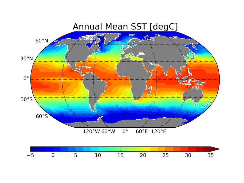
The authors wish to thank Christian Ethé and all the members of the NEMO System Team
     for their collaboration during the implementation of the coupling.
     This document should be cited as:
     Vichi M., Lovato T., Gutierrez Mlot E., McKiver W. (2015). Coupling BFM with Ocean
     models: the NEMO model (Nucleus for the European Modelling of the Ocean). BFM
     Report series N. 2, Release 1.0, August 2015, Bologna, Italy, http://bfm-community.eu, pp.
     31

Copyright 2015, The BFM System Team. This work is licensed under the Creative Commons
Attribution-Noncommercial-No Derivative Works 2.5 License. To view a copy of this license, visit
http://creativecommons.org/licenses/by-nc-nd/2.5/ or send a letter to Creative Commons, 171 Second Street, Suite 300,
San Francisco, California, 94105, USA.

2
Contents

1 Introduction                                                                                                                                5
  1.1 Eulerian coupling . . . . . . . . . . . . . . . . . . . . . . . . . . . . . . . . . . . .                                               5
  1.2 Information flow and numerical integration . . . . . . . . . . . . . . . . . . . . . .                                                  6

2 Technical coupling with NEMO                                                                                                                 9
  2.1 Integration of BFM in the NEMO-TOP interface                .   .   .   .   .   .   .   .   .   .   .   .   .   .   .   .   .   .   .    9
  2.2 BFM and TOP parameters . . . . . . . . . . . .              .   .   .   .   .   .   .   .   .   .   .   .   .   .   .   .   .   .   .    9
  2.3 The flow chart . . . . . . . . . . . . . . . . . . .        .   .   .   .   .   .   .   .   .   .   .   .   .   .   .   .   .   .   .   11
  2.4 Boundary conditions in TOP . . . . . . . . . . .            .   .   .   .   .   .   .   .   .   .   .   .   .   .   .   .   .   .   .   13
  2.5 Coupling of the underwater shortwave irradiance             .   .   .   .   .   .   .   .   .   .   .   .   .   .   .   .   .   .   .   17

3 Installation, configuration and compilation                                                                                                 19
  3.1 Installation . . . . . . . . . . . . . . . . . .    .   .   .   .   .   .   .   .   .   .   .   .   .   .   .   .   .   .   .   .   .   19
  3.2 Configuring BFM with NEMO . . . . . . . .           .   .   .   .   .   .   .   .   .   .   .   .   .   .   .   .   .   .   .   .   .   19
       3.2.1 The GYRE_BFM preset . . . . . . .            .   .   .   .   .   .   .   .   .   .   .   .   .   .   .   .   .   .   .   .   .   20
  3.3 Compilation and interaction with makenemo           .   .   .   .   .   .   .   .   .   .   .   .   .   .   .   .   .   .   .   .   .   21

4 Running GYRE_BFM                                                                                                                            23
  4.1 Description . . . . . . . . . . . . . . . . . . . . . . . . . . . . . . . . . . . . . . .                                               23
  4.2 Serial and parallel simulations . . . . . . . . . . . . . . . . . . . . . . . . . . . . .                                               23
  4.3 Results . . . . . . . . . . . . . . . . . . . . . . . . . . . . . . . . . . . . . . . . . .                                             23

5 The PELAGOS global ocean configuration                                                                                                      25
  5.1 Description . . . . . . . . . . . . . . . . . . . . . . . . . . . . . . . . . . . . . . .                                               25
  5.2 The PELAGOS2 preset . . . . . . . . . . . . . . . . . . . . . . . . . . . . . . . . .                                                   26
  5.3 Results . . . . . . . . . . . . . . . . . . . . . . . . . . . . . . . . . . . . . . . . . .                                             26

6 Output and diagnostics                                                                                                                      29
  6.1 Introduction . . . . . . . . . . . . . . . . . . . . . . . . . . . . . . . . . . . . . . .                                              29
  6.2 Rebuilding the output and restart files . . . . . . . . . . . . . . . . . . . . . . . . .                                               29
  6.3 Diagnostic computation of satellite chlorophyll . . . . . . . . . . . . . . . . . . . .                                                 29

Bibliography                                                                                                                                  31

                                                                                                                                               3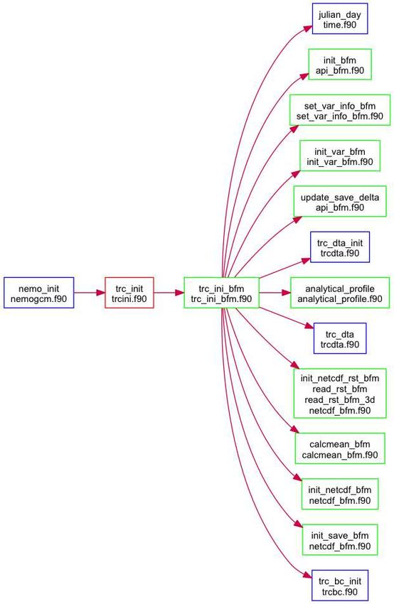
1 Introduction
1.1 Eulerian coupling
This introduction presents the major theoretical assumptions for the Eulerian coupling between a
general circulation model of the ocean (NEMO, Nucleus for the European Modelling of the Ocean,
http://nemo-ocean.eu) and a biogeochemical model of the pelagic system (BFM, Biogeochemical
Flux Model, http://bfm-community.eu). The concepts presented in this section and partly in the more
technical Chap. 2 are to be considered valid for any coupling of the BFM with an ocean general
circulation model (OGCM).
   The BFM is designed as a set of ordinary differential equations that resolve the fluxes of biogeo-
chemical constituents in the marine environment. By construction, it assumes that biological and
chemical variables are homogeneously distributed in the infinitesimal water volume, which is clearly
a poor approximation for living cells and particulate organic matter in general. From a theoretical
point of view, the biological components of the marine environment have always been casted in the
Eulerian representation, using dissolved nutrients and unicellular plankton as models because they are
sufficiently small and passive to be considered “parts” of the fluid. This theoretical formulation has
been proposed initially by O’Brien and Wroblewski (1973), then Robinson (1997) and summarized
in Hofmann and Lascara (1998) and Vichi et al. (2007b). It must be noted that all these formulations
either neglected the role of turbulent diffusive processes or assumed that turbulent fluctuations in the
biological fields are affected by the same Reynolds averaging used for the fluid properties.
   We use the conceptual framework proposed by Vichi et al. (2007b), and we acknowledge that
a similar theoretical formulation was previously proposed by Robinson (1997), who also provided
a mathematical derivation of the analytical solutions. Passively transported variables can be basi-
cally described using concentrations of functional living and non-living components (the chemical
functional families proposed by Vichi et al., 2007b), and we write the conservation equation for an
infinitesimal volume of fluid containing the concentration C for a BFM variable. We apply the con-
tinuum hypothesis that the value of C is a continuous function of space and time. The basic equation
in a fluid is thus:
                                              ∂C
                                                  = −~∇ · ~F,                                    (1.1.1)
                                               ∂t
where ~F is the generalized flux of Ci through and within the basic infinitesimal element of mass of the
fluid. By making the continuum approximation valid for biogeochemistry, we can further separate the
flux in a physical part and a biological reaction term

                                      ∂C
                                         = −~∇ · ~Fphys − ~∇ · ~Fbio .                           (1.1.2)
                                      ∂t
   The second term on the right hand side of (1.1.2) cannot be measured directly because living cells
have finite dimensions, and therefore we assume that it can be approximated with the following eule-
rian approach:
                                    ~∇ · ~Fbio = −wB ∂ C + ∂ C     .                          (1.1.3)
                                                     ∂z    ∂ t bio

                                                                                                      5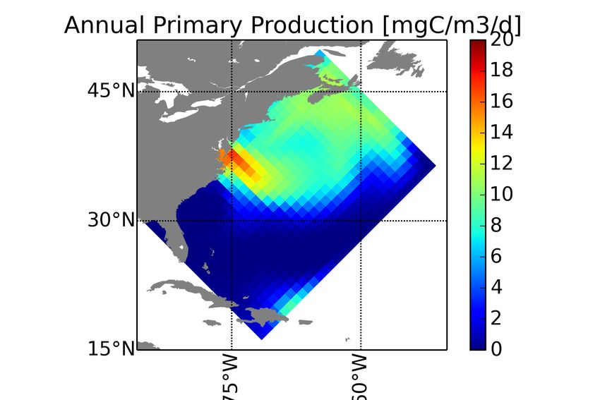
1 Introduction

   Both terms in eq. (1.1.4) represent the biogeochemical divergence flux and parameterize the sinking
of biological particulate matter and the local time rate of change due to biogeochemical transformation
processes. The sinking velocity wB is introduced for those state variables that have a mass-related
vertical velocity other than the fluid vertical velocity.
   This approximation brings us to the typical form of an advection-diffusion-reaction equation in an
incompressible fluid:

                   ∂C                             ∂   ∂C      ∂C ∂C
                      = −u · ∇C + ∇H · (AH ∇H C) + AV    − wB    +                               (1.1.4)
                   ∂t                             ∂z ∂z       ∂z   ∂t             bio

where u ≡ (u, v, w) is the three-dimensional current velocity and (AH , AV ) are the horizontal and ver-
tical turbulent diffusivity coefficient for tracers. To highlight the coupling between physical and bio-
geochemical processes, we may rewrite this equation in component forms, also indicating the ocean
variables that are resolved by the OGCM and needed for the reaction term R:

      ∂C    ∂C    ∂C    ∂C                   ∂   ∂C      ∂C
         +u    +v    +w    = ∇H · (AH ∇H C) + AV    − wB    + R (T, S, W, E)                     (1.1.5)
      ∂t    ∂x    ∂y    ∂z                   ∂z ∂z       ∂z
where the scalar symbols in the last term indicate water temperature (T), salinity (S), the intensity of
wind (W), and shortwave irradiance (E).

1.2 Information flow and numerical integration
Equation (1.1.4) is one approximated form of a primitive equation for biogeochemical variables in
the ocean and requires the knowledge of ocean physical variables to be solved. The time evolution
of physical variables is carried out by the OGCM and transferred to the biogeochemical model. A
typical, generic scheme of the information flow between the two models is presented in Fig. 1.1. The
physical variables are used to compute the advection, diffusion and reaction terms in eq. (1.1.4) and
then combined to obtain the forward in time biogeochemical states. This equation cannot be solved
analytically but requires a numerical integration, just as it happens for temperature and salinity on
OGCM. Usually, the same kind of numerical scheme is used. The sensitivity of the BFM to integration
schemes has been tested by Butenschön et al. (2012), and it was concluded that the source splitting
method is more accurate. Currently, NEMO uses a time integration based on source splitting with a
leapfrog scheme for active tracers (Madec, 2008); in the case of BFM-NEMO the final integration is
carried out with a simple Euler-forward step, but still with source splitting .

6
1.2 Information flow and numerical integration

Figure 1.1: Scheme of the information flow between the ocean model and the biogeochemical state
            variables. The blue boxes indicate that the computation is carried out directly by the
            OGCM or using modified routines belonging to the OGCM. Integrator is a generic name
            for the solver used to advance in time the solution of the coupled physical-biogeochemical
            system.

                                                                                                    7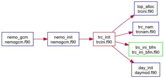
2 Technical coupling with NEMO
2.1 Integration of BFM in the NEMO-TOP interface
BFM and NEMO are separated codes that are maintained by different groups of developers. The
coupled configuration is therefore the result of a joint compilation of the two codes, where the BFM
is a modular external library of NEMO. This document assumes that you are already familiar with
NEMO and it does not substitute the NEMO documentation (Madec, 2008) which should be used as
reference for the specific namelist parameters and code macros.
   NEMO contains an interface for the computation of biogeochemical tracers named TOP (from
the French Traceurs Oceanographique Passives) which is contained in the TOP_SRC directory of
NEMO code. This interface allows to use all the same numerical schemes available for the active
tracers to solve the advective and diffusive processes, as well as to prescribe surface, bottom and
lateral boundary conditions. This is a crucial requirement for the inclusion of BFM in any OGCM,
and it is possible because all NEMO routines have been written with explicit input-output arguments
to pass either temperature or salinity or biogeochemical tracers.
   The BFM has been integrated in this framework with the addition of a seamless software layer that
uses the generic tracer interface called MY_TRC. In addition, the BFM source code provides all the
ancillary routines that are required for the coupling in the directory $BFMDIR/src/nemo. When
a NEMO configuration containing the BFM is compiled, this generic tracer interface is activated and
the external directory containing the BFM coupling interface is included, substituting some of the
standard routines contained in TOP_SRC. The compilation of the coupled system is done with the
BFM configuration script detailed in Sec. 3.2.
   This is activated with the macro key_my_trc and the BFM is plugged into the NEMO flow chart
during the initialization and stepping phases. It important to make clear that BFM still uses its own
libraries for diagnostic output and restart files.

2.2 BFM and TOP parameters
The biogeochemical processes of the BFM are controlled by their own namelist files as described in
the manual (Vichi et al., 2015), but when run in coupled configuration there are some additional pa-
rameters derived from the NEMO TOP namelist that must be adjusted. Particularly, this occurs for the
prescription of initial and boundary conditions because both rely on the NEMO facilities for reading
and interpolating external files. The file namelist_top_cfg generated by the BFM configuration
script (see Sec. 3.2) contains the namelist namtrc_dta which gives the information on the initial
data values for the BFM variables:
!-------------------------------------------------------------------------!
!NAMELIST namtrc_dta
!-------------------------------------------------------------------------!
!   Initialisation from data input file
!   for each BFM variable set the structure sn_trcdta(VARNAME)
!   and the conversion factor rn_trfac(VARNAME)
!   Specifications for fld_read:
!   !file name!frequency (hr)!variable!time interp.!clim !’yearly’ or !weights !rotation!land/sea
!   !         !(if
2 Technical coupling with NEMO

&namtrc_dta
  sn_trcdta(O2o)     = ’data_1m_O_nomask’, -12 , ’O2’ , .false. , .true. , ’yearly’ , ’’, ’’, ’’
  sn_trcdta(N1p)     = ’data_1m_P_nomask’, -1  , ’PO4’ , .false. , .true. , ’yearly’ , ’’, ’’, ’’
  rn_trfac(O2o)      =   22.4 ! conversion factor from ml/l to mmol m3 (1 mol O2 = 22.4 l)
  rn_trfac(N1p)      =   1.0   ! no conversion
...
  cn_dir         =   ’./’      !   root directory for the location of the data files
/

   The parameters of the fld_read structure sn_trcdta allow to specify the name of the file, the fre-
quency of input data and the interpolation weights. Note that the interpolation is still two-dimensional
only and the input data must already be on the vertical grid of the model. It is possible to give a
conversion factor that may also be used to increase artificially the initial values of a uniform factor.
The BFM named constants for the variables are substituted by the configuration script at compilation
time and then copied to the running directory as fully detailed in Sec. 3.2.
   In addition to this part that is common to other biogeochemical models in the TOP interface,
the BFM allows to choose the specific mode of initialization for each variable in the namelist
bfm_init_nml. This is the same namelist used for the STANDALONE model as described in Vichi
et al. (2015) but when coupled with NEMO it also allows to specify if each variable should start from
the initial file given in the namelist above, from a constant homogeneous value or from an analytical
profile:
!-------------------------------------------------------------------------!
! NAMELIST bfm_init_nml
!-------------------------------------------------------------------------!
!Pelagic initialisation of standard variables
!0 =
!
! Initialization with InitVar structure
!----------------------------------------
! NOTE:
! This part is still experimental and will be improved in the future
!----------------------------------------
! BFM variable information for data input
! available fields:
! integer init: select the initialization
!               0 = homogeneous
!               1 = analytical
!               2 = from file
! options for init==1
!   real anv1: value in the surface layer
!   real anz1: depth of the surface layer
!   real anv2: value in the bottom layer
!   real anz2: depth of the bottom layer
! options for init==2
! * Options currently used when coupled with NEMO
!   logical obc: variable has open boundary data
!   logical sbc: variable has surface boundary data
!   logical cbc: variable has coastal boundary data
! * Options not used when coupled with NEMO because
!   overridden by values in namelist_top_cfg
!   char filename: name of the input file
!   char varname: name of the var in input file
!-------------------------------------------------------------------------!
&bfm_init_nml
   InitVar(O2o)%init = 0
   O2o0 = 300.0,
   InitVar(N1p)%init = 2
   InitVar(N1p)%sbc = .false.
   InitVar(N1p)%cbc = .false.
   InitVar(N1p)%obc = .false.
   InitVar(N1p)%init = 1
   InitVar(P1c)%anv1 = 5.0
   InitVar(P1c)%anz1 = 20.0

10
2.3 The flow chart

    InitVar(P1c)%anv2 = 1.0
    InitVar(P1c)%anz2 = 100.0
\

   In the above example, oxygen is initialized with a constant value, phosphate is read from file and
phytoplankton carbon is initialized with a stepwise analytical profile with higher concentration in the
surface 20 m, a lower value in the adjacent 100 m and the background concentration in the reminder
of the water column.
   Surface, coastal and open boundary values for biogeochemical variables can also be switched on
and off from this namelist and they are fully detailed in Sec. 2.4.
   Another important parameter to be checked in coupled configurations is the sinking velocity
of BFM variables. BFM computes a dynamical sinking velocity for phytoplankton that is de-
pendent on nutrient stress (if activated) and a constant background sinking rate for phytoplankton
and detritus. These are considered to be global variables and they are included in the namelist
PelGlobal_parameters:
!-------------------------------------------------------------------------!
!NAMELIST PelGlobal_parameters
!-------------------------------------------------------------------------!
! Sinking rates of Pelagic Variables
! : for mem_PelGlobal filled by InitPelGlobal
! NAME           UNIT      DESCRIPTION
! p_rR6m         [m/d]   detritus sinking rate
! KSINK_rPPY      [m]    prescribe sinking rate for phytoplankton below this
!                        depth threshold to p_rR6m value. Use 0.0 to disable.
! AggregateSink logic    use aggregation = true to enhance the sink rate
!                        below a certain depth and bypass the prescribed
!                        sinking
! depth_factor    [m]    depth factor for aggregation method
!-------------------------------------------------------------------------!
&PelGlobal_parameters
  p_rR6m         = 10.0
  KSINK_rPPY     = 150.0
  AggregateSink = .FALSE.
  depth_factor   = 2000.0
/

   The coupling with NEMO adds three parameters that allow to parameterize the change in the
sinking rate at depth. Below a certain depth, it is assumed that aggregation takes place. This is
parametrized either by imposing the sinking rate of detritus to phytoplankton concentration below a
fixed depth KSINK_rPPy (in meters), or by activating the enhancement of background velocity also
found in the PISCES model of NEMO (AggregateSink = .TRUE.).

2.3 The flow chart
The BFM is zero-dimensional by construction and defined only in the ocean points. This implies that
the BFM memory is one dimensional, with all the land points stripped out from the 3D domain and
the remapping into the ocean grid is done only when dealing with transport processes (as shown in
Fig. 2.1 taken from the BFM manual).
   The flow of information between NEMO and the BFM is presented using “butterfly” graphs that
show the main caller of the function of interest and the tree of calls. By convention, the routines of
NEMO are indicated with blue boxes while the BFM routines are in green. Routines indicated with
red boxes originally belong to NEMO TOP_SRC but are substituted by the ones provided in the BFM
directory ($BFMDIR/src/nemo).

                                                                                                    11
2 Technical coupling with NEMO
Figure 2.1: Layout of the main memory array for the pelagic variables and schematic of the remapping
into the NEMO three-dimensional ocean grid for transport processes (see Vichi et al., 2015
for a description of the code naming).
122.4 Boundary conditions in TOP
Figure 2.2: Graph of the initialization routine for passive tracers. This routine is not the default TOP
routine but it is substituted by the version contained in $BFMDIR/src/nemo that con-
tains the call to the BFM routine trc_ini_bfm.
A scheme of the NEMO initialization of passive tracers is shown in Fig. 2.2, where a specific routine
was designed to handle the information flow toward BFM (trc_ini_bfm). The initialization of
BFM (Fig. 2.3) in the coupling is different from the STANDALONE configuration, because it includes
also the transfer of grid parameters from NEMO and the reading of three-dimensional field data of
initial conditions (see Sec. 2.4).
The time marching computation in NEMO are performed in the stp routine (Fig. 2.4) and the
passive tracers are specifically addressed in trc_stp. A modified version of the latter subroutine
was created to include three different routines for the solution of BFM core processes (trc_bfm),
the advection and diffusion of state variables (trc_trp_bfm), and the computation of output data
(trc_dia_bfm). In particular, the trc_bfm routine includes the retrieval of environmental condi-
tions from NEMO (envforcing_bfm), like e.g., temperature, salinity, light, and the computation
of BFM biogeochemical processes (EcologyDynamics).
The transport of BFM state variables is operated by trc_trp_bfm subroutine (Fig. 2.5), which
is derived from the general one of NEMO for passive tracers (namely, trc_trp). In fact, this sub-
routine also handles the application of external boundary conditions (trc_bc_bfm), vertical sink-
ing (trc_set_bfm) and it prepares the model variables to perform the Euler Forward integration
(trc_nxt_bfm).
.
2.4 Boundary conditions in TOP
Since version 3.6, NEMO allows to define different types of boundary conditions for biogeochemical
tracers. For every single variable it is possible to define a field of surface boundary conditions, such as
deposition of dust or nitrogen, which is then interpolated to the grid and timestep using the fld_read
function. The same facility is available to include river inputs (coastal boundary conditions) and it is
under development the treatment of open boundary conditions.
The namelist namtrc_bc is contained in file namelist_top_cfg (which in the BFM is gen-
erated during the first compilation, see Sec. 3.2) and allows to specify the name of the files, the
132 Technical coupling with NEMO
Figure 2.3: Butterfly graph of the BFM initialization within NEMO.
142.4 Boundary conditions in TOP
Figure 2.4: Graph of the stepping routine trc_stp for passive tracers. This routine is not the default
TOP routine but it is substituted by the version contained in $BFMDIR/src/nemo that
contains the calls to the BFM routines trc_bfm, trc_trp_bfm and trc_dia_bfm.
frequency of the input and the time and space interpolation as done for any other field using the
fld_read interface. It also allows to specify how freshwater fluxes from sea ice freezing and melt-
ing affect the concentration of tracers.
!-------------------------------------------------------------------------!
!NAMELIST namtrc_bc
!-----------------------------------------------------------------------
! Set input files for surface (s), coastal (c) or open (o) boundary
! conditions for each variable
! sn_trc?bc(VARNAME): structure with file name and interpolation
! rn_tr?fac(VARNAME): conversion factor
! Specifications for fld_read:
! !file name!frequency (hr)!variable!time interp.!clim !’yearly’ or !weights
!rotation!land/sea
! ! !(if2 Technical coupling with NEMO
Figure 2.5: Call graph of the transport routine trc_trp_bfm for BFM tracers.
162.5 Coupling of the underwater shortwave irradiance
2.5 Coupling of the underwater shortwave irradiance
One of the largest coupling mechanism between ocean physics and biogeochemistry is the irradiance
attenuation driven by suspended and dissolved components (e.g. Patara et al., 2012). In NEMO this is
controlled by the namelist namtra_qsr, which is usally not modified in the configuration files and
it is located in namelist_ref
!-----------------------------------------------------------------------
&namtra_qsr ! penetrative solar radiation
!-----------------------------------------------------------------------
sn_chl =’chlorophyll’, .......
cn_dir = ’./’ ! root directory for the location of the runoff files
ln_traqsr = .true. ! Light penetration (T) or not (F)
ln_qsr_rgb = .true. ! RGB (Red-Green-Blue) light penetration
ln_qsr_2bd = .false. ! 2 bands light penetration
ln_qsr_bio = .false. ! bio-model light penetration
nn_chldta = 1 ! RGB : Chl data (=1) or cst value (=0)
rn_abs = 0.58 ! RGB & 2 bands: fraction of light (rn_si1)
rn_si0 = 0.35 ! RGB & 2 bands: shortest depth of extinction
rn_si1 = 23.0 ! 2 bands: longest depth of extinction
ln_qsr_ice = .true. ! light penetration for ice-model LIM3
/
The coupling with a biogeochemical model is controlled by the parameter ln_qsr_bio. If this is
set to false as in the default settings above, shortwave radiation penetrates the interior of the ocean ac-
cording to a 4 waveband algorithm (ln_qsr_rgb=.true.), where the incident spectrum is decom-
posed in infrared, red, green and blue (RGB) portions that are attenuated differentially as a function
of chlorophyll concentration. This approximated tabulated solution has been proposed by Lengaigne
et al. (2007) using original data by Morel (1988) for 68 wavelengths. If available for the specific
configuration, the chlorophyll field is read from a data file (given in the structure sn_chl) and used
to compute the attenuation coefficients for RGB and the shortwave radiation that is absorbed at every
level. This information is used to compute the trend of ocean temperature. The alternative uncupled
configuration is the standard formulation by Paulson and Simpson (ln_qsr_2bd=.true.) where
light is attenuated according to a 2 waveband formulation, near-infrared and visible.
In both of the cases above the BFM is not coupled to NEMO, that is the evolution of BFM
chlorophyll does not feedback into the physical model to determine the vertical divergence of the
shortwave field. When ln_qsr_bio=.true., the control of light propagation is completely
passed to the BFM (PAR_parameters in Pelagic_Environment.nml) and the namelist
above is not considered. The infrared attenuation depth is substituted by the attenuation coef-
ficient (p_epsIR=1/rn_si0) and the fraction of visible light spectral energy is equivalent to
p_PAR=1-rn_abs:
!-------------------------------------------------------------------------!
! PAR_parameters
!-------------------------------------------------------------------------!
&PAR_parameters
...
p_PAR = 0.42
p_epsIR = 2.857
...
/
The difference between a coupled and uncoupled simulation depends on two factors: how different the
chlorophyll seasonality is from the climatological dataset used to compute the attenuation coefficient
and the vertical distribution of dynamical chlorophyll, because the satellite-derived chlorophyll is
assumed to be homogeneous in the vertical. An example of the difference in the resulting shortwave
flux at every depth is given in Fig. 2.6 for a station in the North Pacific (Station PAPA).
172 Technical coupling with NEMO
Figure 2.6: Difference of shortwave heat flux between an uncoupled and coupled simulation, where
light attenuation is a function of the BFM chlorophyll.
183 Installation, configuration and compilation
3.1 Installation
Both the BFM and NEMO codes have to be downloaded from the respective distribution sites. The
coupling is officially maintained from NEMO version 3.6 and BFM version 5.1. Please contact the
BFM System Team (bfm_st@lists.cmcc.it) for information on the use of BFM with the sta-
ble version of NEMO 3.4.1. In the following, it is assumed that the NEMO code is found in a directory
identified by the environmental variable $NEMODIR and the BFM in the directory $BFMDIR.
As it occurs for the NEMO compilation, it is necessary to select a configuration before doing
the compilation of BFM-NEMO. The default basic configuration of BFM coupled with NEMO is
GYRE_BFM (Chap. 4), which simulates the general circulation of a double gyre ideally located in
the north-western Atlantic. The directory GYRE_BFM is already distributed with NEMO 3.6 (and
above) in the directory NEMOGCM/CONFIG, while the global ocean configuration PELAGOS (see
Chap. 5) is provided with the BFM and other coupled configurations can be added by the user.
Refer to the NEMO web site for how to obtain the code and how to install it. It is suggested to first
compile and run the desired NEMO configuration without the BFM, in order to set up the necessary
compilation environment. The same architecture file contained in the directory NEMOGCM/ARCH will
in fact be used by the BFM configuration script. The same software required for running NEMO is
necessary for the coupled configuration, with the only addition of perl (version 5.8.2 and above),
which is used automatically during compilation time to generate the code.
Download the source code from the BFM website or through the git repository. In the example
below it is assumed that you downloaded the tarball. The downloaded file may have a different name
based on the version. As a final step create the required basic environmental variables pointing at the
root directories as:
% mkdir $HOME/BFM
% cd $HOME/BFM
% gunzip bfm-release-.tgz
% tar xvf bfm-release-.tar
% export BFMDIR=$HOME/BFM
% export NEMODIR=$HOME/NEMO
3.2 Configuring BFM with NEMO
Configuration and deployment of the model is done automatically by the script bfm_configure.sh (see
the BFM manual for more information or simply run ./bfm_configure.sh -h). The default
configuration (see Chap. 4) is generated, compiled and deployed with the command:
% cd $BFMDIR/build
% ./bfm_configure.sh -gcd -a ARCHFILENAME -p GYRE_BFM
where ARCHFILENAME must be substituted by the name of your specific architecture files
that is found in NEMOGMC/ARCH. The generated namelists and model executable will be found
193 Installation, configuration and compilation
in $BFMDIR/run/gyre_bfm or in the directory indicated by the environmental variable
$BFMDIR_RUN if set.
3.2.1 The GYRE_BFM preset
As it occurs for BFM STANDALONE, a configuration is defined by a model lay-
out structure and initial input values. The GYRE_BFM preset is found in the
$BFMDIR/build/configurations/GYRE_BFM folder and contains the following files:
configuration: compilation and deployment options
This file uses the F90 namelist format to set values and strings must be surrounded by the ’ character:
&BFM_conf
MODE = ’NEMO’,
CPPDEFS = ’BFM_PARALLEL INCLUDE_PELCO2 INCLUDE_PELFE INCLUDE_DIAG’,
ARCH = ’ARCHFILENAME’,
PROC = 8,
EXP = ’gyre_bfm’,
QUEUE = ’poe_short’,
EXPFILES = ’iodef.xml namelist_cfg namelist_top_cfg’
/
These options prescribe that the GYRE_BFM configuration is a coupled MODE with NEMO, and it
has the pre-compiler macros specified in CPPDEFS (parallel simulation, as it is in the standard NEMO
GYRE configuration; inclusion of carbonate and iron dynamics and possibility to store the diagnostic
output). In particular, the BFM_PARALLEL macro is used to enable the creation of a simulation log
file when using parallel execution on multiple processors. Please refer to the BFM manual (Vichi
et al., 2015) for further details on the other macros.
The coupled configurations also require to include the parameters to run the OGCM in the running
directory. This is done by means of the variable EXPFILES, that contains the name of the ancillary
files (the configuration namelist for NEMO and TOP interface), as well as the the I/O definition
that have to be copied to the running directory.The configuration script also copies the reference
configurations from the CONFIG/SHARED directory of NEMO.
layout: memory layout configuration file
This file contains the list of state variables defined in the BFM. This is independent of the coupled
configuration and it is fully detailed in the BFM manual (Vichi et al., 2015).
namelists_bfm: template namelist file for BFM and NEMO-TOP with standard
values
This file contains all the standard values of the namelists used for the experiment. This file is processed
by the configuration script and the BFM named constants are substituted by numerical constants both
for BFM parameters and for the ones needed by NEMO-TOP, such as the boundary conditions (see
Sec. 2.4), generating the configuration namelist file namelist_top_cfg. Namelists are checked
for consistency against the source code at generation time and the files effectively used for the simula-
tion are copied to the $BFMDIR/run directory. The regular user will generally work with generated
namelists and usually there is no need to change any keyword in this file unless new boundary condi-
tions are added or the layout is changed.
203.3 Compilation and interaction with makenemo
3.3 Compilation and interaction with makenemo
This section provides more details on the joint compilation and it is intended mostly for NEMO
developers. The configuration script, when called with MODE option equal to NEMO, pre-
pares the BFM code and make it compatible with the NEMO compilation using the FCM con-
figuration manager (http://www.metoffice.gov.uk/research/collaboration/fcm). More specifically,
bfm_configure.sh creates an fcm file for the BFM source code that is then included in the
compilation process by means of the NEMOGCM/CONFIG/GYRE_BFM/cpp_GYRE_BFM.fcm file
(or any other cpp_* file from a coupled BFM configuration, see for instance Chap. 5):
bld::tool::fppkeys key_dynspg_flt key_ldfslp key_zdftke key_vectopt_loop
key_top key_my_trc key_mpp_mpi key_iomput
inc $BFMDIR/src/nemo/bfm.fcm
The file bfm.fcm does not exist initially in the BFM tree and it is generated from a template found
in $BFMDIR/build/scripts/proto depending on the directory structure and model choices.
The specific pre-compilation macro BFM_NEMO that is required by BFM to activate the NEMO-
related parts of the code is also added to the list of macros.
Finally, the compilation with makenemo is launched by prescribing the use of an external di-
rectory (option -e, introduced since version 3.5) that allows the substitution of the TOP_SRC files
with the ones containing the coupling with the BFM (see Chap. 2). After the first genera-
tion with the bfm_configure.sh script it is also possible to compile the model from the standard
NEMOGCM/CONFIG directory with the command
./makenemo -n GYRE_BFM -m ARCHFILE -e ${BFMDIR}/src/nemo
214 Running GYRE_BFM
4.1 Description
GYRE_BFM is an analytical configuration of NEMO that simulates a warm and cold gyre ideally
located in the North Atlantic. Only the pelagic system can be currently simulated with this configura-
tion. The model is forced with analytical heat and momentum fluxes over a regular year of 360 days
and starts from homogeneous initial conditions for biogeochemistry. The model output is in NetCDF.
The default grid is 22 x 32 with 31 vertical levels.
4.2 Serial and parallel simulations
GYRE_BFM is the simplest example to run as a single process on a desktop computer because
the grid is rather coarse. However, the default GYRE configuration in NEMO is set up to use
parallel computation and the advanced XIOS server (http://www.nemo-ocean.eu/Using-NEMO/User-
Guides/Basics/XIOS-IO-server-installation-and-use). To compile in serial mode it is necessary to re-
move the macro key_mpp_mpi for parallel computation that is found in $NEMODIR/NEMOGCM/-
CONFIG/GYRE_BFM/cpp_GYRE_BFM.cpp. It is also possible to use the standard NEMO output
instead of the XIOS library by removing the macro key_iomput in the cpp file of the configuration.
Together with the BFM, the GYRE configuration increases substantially the computational burden,
therefore it is also a good example to learn how to use the model with multiple processes. In this case,
it is necessary to install an MPI library (like http://www.open-mpi.org/) and use a NEMO ARCH file
with the mpif90 compiler. When GYRE_BFM is run in parallel, the BFM netcdf output is produced
for each sub-domain just like it happens for NEMO and the same naming convention is used. The
output can be “rebuilt”, that is all the tiles are combined together, to obtain the full domain using the
tool described in Sec 6.2.
4.3 Results
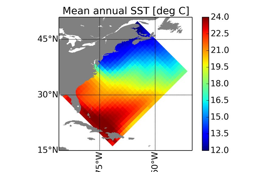
This example demonstrates the role of the major physical factors in driving the plankton response.
The double gyre is characterized by a warm subtropical cell and a cold subpolar cell (Fig. 4.1) that
are separated by a simplified current that should mimic the features of a western boundary current.
Phytoplankton production is generally localized around the current bordering the gyres and in corre-
spondence with the cold and less stratified parts of the sub-polar gyre.
234 Running GYRE_BFM
Figure 4.1: Example output from GYRE_BFM after 9 years of simulation. Mean annual sea surface
temperature (top) and net primary production (bottom).
245 The PELAGOS global ocean configuration
5.1 Description
PELAGOS stands for PELAGic biogeochemistry for Global Ocean Simulations (Vichi et al., 2007a)
and it is a global ocean implementation of the BFM with NEMO using the family of ORCA grids.
It was originally designed as a specific sub-set and integration of functional parameterizations that
were required to address global ocean dynamics (see Vichi et al. (2007b)), but it is now intended
to be just another configuration of the BFM. This implies that any BFM feature can now be used
with NEMO also in global ocean configurations. The PELAGOS family of configurations follows the
ORCA family specifications, that is PELAGOS2 refers to the ORCA2 grid, PELAGOS1 to ORCA1
and so forth.
PELAGOS2 is the coarsest global ocean resolution but still requires a parallel computing en-
vironment for its usage. One needs to have a fully functioning NEMO implementation of the
ORCA2_LIM configuration before attempting to run PELAGOS2 (see details here: http://www.nemo-
ocean.eu/Using-NEMO/Configurations/ORCA2_LIM_PISCES). The default set up is the same as
ORCA2_LIM with the following features:
• sea ice model LIM2 (key_lim2)
• filtered linear free surface (key_dynspg_flt)
• Laplacian diffusion with isopycnal diffusion (key_ldfslp) and coefficients for horizontal dif-
fusion with 2-D variation (key_traldf_c2d)
• eddy-induced velocity parameterization of enhanced diffusion (key_traldf_eiv) and re-
lated diagnostics (key_diaeiv)
• coefficients for horizontal viscosity with 3-D variation (key_dynldf_c3d)
• vertical turbulence TKE closure and vertical tidal mixing (key_zdftke and key_zdftmx)
• bottom boundary layer parameterization (key_trabbl)
• double diffusion (key_zdfddm)
with the addition of the pre-processing macros to turn on passive tracers and the BFM (key_top and
key_my_trc)
By default, PELAGOS2 is compiled with the embedded I/O library XIOS (key_iomput) which
must be compiled as an external library. On a modern super-computer, 1 month of simulation takes
about 5 minutes using 128 processors.
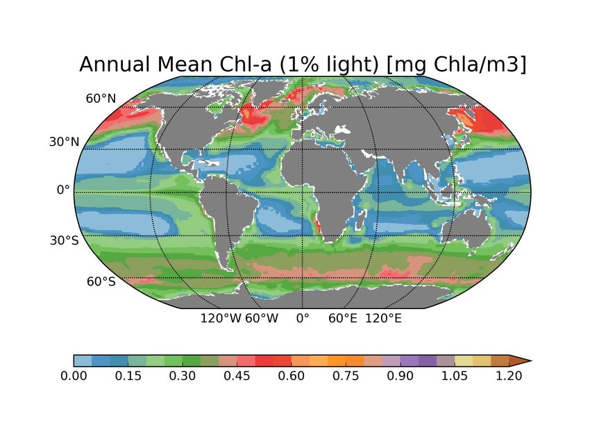
255 The PELAGOS global ocean configuration 5.2 The PELAGOS2 preset This preset is not part of the official NEMO release but uses the makenemo tool to create the config- uration PELAGOS2 in the $NEMODIR/NEMOGCM/CONFIG directory to allow the compilation with FCM. Users should know that the file cpp_PELAGOS2.fcm containing the preprocessing macros listed above is found in this directory, and once you have created the corresponding configuration directory in the NEMO tree it will be copied there and should be subsequently modified from there. When the configuration script is called with the PELAGOS2 preset, makenemo is requested to create a new configuration and % ./bfm_configure.sh -gcd -a ARCHFILE -p PELAGOS2 You are installing a new configuration Creating PELAGOS2/WORK = OPA_SRC TOP_SRC LIM_SRC_2 for PELAGOS2 MY_SRC directory is : PELAGOS2/MY_SRC .... The run directory is created in $BFMDIR_RUN/pelagos2 just like all other BFM presets and the nemo executable is linked to there. 5.3 Results A 9 years-long simulation was performed with the PELAGOS2 configuration by using the normal year CORE II atmospheric forcing (Large and Yeager (2009)) and climatological river runoff (Dai and Trenberth (2002)) and nutrients loads (Cotrim da Cunha et al. (2007)). All data are available on the NEMO web site (http://www.nemo-ocean.eu/Using-NEMO/Configurations/ORCA2_LIM_PISCES). The initial conditions of both physical and biogeochemical variables were set using the World Ocean Atlas 2009 climatological fields (NESDIS NOAA Atlas (2010)). In Fig. 5.1 are shown the mean an- nual fields for the sea surface temperature and the satellite-like chlorophyll concentration (using 1% light threshold for depth integration, see Sec. 6.3) computed in the last year of simulation. PELA- GOS2 is capable to reproduce the main distribution patterns of primary producers across the different oceanic regions, by preserving also the minimum concentration within the subtropical oceanic gyres. 26
5.3 Results

Figure 5.1: Example output from PELAGOS2 after 9 years of simulation. Mean annual surface tem-
            perature (top) and satellite-like chlorophyll at 1% light level (bottom). See Sec. 6.3 for
            satellite-like chlorophyll computation.

                                                                                                   27
6 Output and diagnostics
6.1 Introduction
BFM uses its own libraries for NetCDF output that are specifically built to create diagnostic rates
between the biogeochemical variables (see Chap. 6 in Vichi et al., 2015). One new feature of NEMO
3.6 is the availability of the external library XIOS, which allows to use an external I/O server and
distribute the computation and preparation of output over different processes and with a different
domain decomposition. The XIOS library functions cannot be used with the BFM yet, therefore it is
needed to post-process the output before accessing the three-dimensional domain fields.
6.2 Rebuilding the output and restart files
The BFM is by construction defined only in the ocean grid points and the output file consists of a one-
dimensional vector. It is therefore required to post-process the output to obtain the three-dimensional
fields on the ocean model grid.
This operation is done with the tools bnremap and bnmerge found in the $BFMDIR/tools
directory:
• bnremap works with a serial single-domain simulation, while
• bnmerge must be used when the model is run in parallel mode. In this case the model produces
one output file per domain containing a vector with the ocean grid points of that specific domain
only and the domains must be merged together to obtain the full domain.
Both applications are controlled with a namelist (see the examples contained in each tool folder),
where it is possible to specify the list of variables to be remapped and the names of the files.
In the case of restart files, it is also possible to use the tool bnmerge to build a single restart file
which may turn to be useful in the case a user want to restart an experiment but with a different number
of parallel processes. The reading of restart input files is controlled by the option bfm_init in the
BFM_General.nml namelist file, which can be set to 0 = no restart, 1 = multiple restart files (one
per process), 2 = restart is a single merged file.
6.3 Diagnostic computation of satellite chlorophyll
This tool is available in directory $BFMDIR/tools/chlsat and computes the chlorophyll concentration
as seen by satellite considering:
1. the optical depth and a tolerance level as described in eq. 2 of Vichi et al. (2007b);
2. the 1% light level;
3. the 0.1% light level
296 Output and diagnostics Input files are the chlorophyll concentration (variable Chla) and the attenuation coefficient (variable xEPS), both with the same number of time stamps, and the mask file. It also allows to compute the attenuation coefficient using the BFM formula from total chlorophyll concentration, background attenuation and chlorophyll-specific absorption coefficient but neglecting the contribution from inor- ganic suspended matter and detritus. This tool also computes the integrated primary production (gross and net) down to 1% and 0.1% light level by setting the flag compute_intpp and providing the paths to the files containing the BFM diagnostics ruPPYc (gross primary production) and resPPYc (respiration). The input parameters are in the namelist chlsat.nml: !------------------------------------------------------------------------------------! !Main initialisation and output specifications !NAME KIND DESCRIPTION !out_fname string Name of output file !inp_dir string Path to the input files !out_dir string Path to the output file !mask_fname string Full path to NEMO mesh_mask file !chla_fname string Name of data file containing 3D Chl !chla_name string Name of Chl variable in file !compute_chlsat logical Compute chlsat (true by default useful only for NPP) !compute_eps logical Use attenuation coefficient from output ! or computed using the BFM formula from Chl ! concentration, neglecting ISM and detritus ! The computation requires: ! p_eps0 real background attenuation of water (m-1) ! p_epsChla real specific attenuation of Chla (m2/mg Chl) ! !eps_fname string Name of data file containing 3D att. coeff. !eps_name string Name of attenuation coeff. variable in file !tolerance real multiplicative factor for optical depth ! ! !compute_intpp logical Compute integrated GPP and NPP down to 1% and 0.1% !gpp_fname string Name of data file containing 3D GPP !gpp_name string Name of GPP variable in file !rsp_fname string Name of data file containing 3D RSP !rsp_name string Name of RSP variable in file !------------------------------------------------------------------------------------! &chlsat_nml out_fname=’chlsat.nc’ inp_dir=’.’ out_dir=’.’ mask_fname=’ORCA2_chlmask.nc’ chla_fname=’bfm_output.nc’ chla_name=’Chla’ compute_chlsat=.true. compute_eps=.false. p_eps0=0.0435 p_epsChla=0.03 eps_fname=’bfm_output.nc’ eps_name=’xEPS’ tolerance=0.0 compute_intpp=.false. gpp_fname=’bfm_output.nc’ gpp_name=’ruPPYc’ rsp_fname=’bfm_output.nc’ rsp_name=’resPPYc’ / 30
Bibliography
Butenschön, M., Zavatarelli, M., Vichi, M., 2012. NESDIS NOAA Atlas, 2010. World ocean atlas
  Sensitivity of a marine coupled physical bio-      2009. Tech. rep., NOAA.
  geochemical model to time resolution, integra-
  tion scheme and time splitting method. Ocean O’Brien, J., Wroblewski, J., 1973. On advection
  Modelling 52–53, 36—53.                            in phytoplankton models. J. Theor. Biology 38,
                                                     197–202.
Cotrim da Cunha, L., Buitenhuis, E., Quéré, C. L.,
  Giraud, X., Ludwig, W., 2007. Potential impact Patara, L., Vichi, M., Masina, S., Fogli, P. G.,
  of changes in river nutrient supply on global      Manzini, E., 2012. Global response to solar ra-
  ocean biogeochemistry. Global Biogeochemi-         diation absorbed by phytoplankton in a cou-
  cal Cycles 21 (4), GB4007.                         pled climate model. Clim. Dyn. 39 (7-8), 1951–
                                                     1968.
Dai, A., Trenberth, K., 2002. Estimates of fresh-
  water discharge from continents: Latitudinal Robinson, A. R., 1997. On the theory of advec-
  and seasonal variations. Journal of Hydrome-       tive effects on biological dynamics in the sea.
  teorology 3, 660–687.                              Proceedings of the Royal Society of London A:
                                                     Mathematical, Physical and Engineering Sci-
Hofmann, E., Lascara, C., 1998. Overview of          ences 453 (1966), 2295–2324.
  interdisciplinary modeling for marine ecosys-
                                                   Vichi, M., Gutierrez Mlot, G. C. E., Lazzari, P.,
  tems. In: Brink, K., Robinson, A. R. (Eds.),
                                                     Lovato, T., Mattia, G., McKiver, W., Masina,
  The Sea. Vol. 10. John Wiley and Sons, pp.
                                                     S., Pinardi, N., Solidoro, C., Zavatarelli, M.,
  507–540.
                                                     July 2015. The Biogeochemical Flux Model
Large, W. G., Yeager, S. G., 2009. The global cli-   (BFM): Equation Description and User Man-
  matology of an interannually varying air–sea       ual. BFM version 5.1. BFM Report Series 1,
  flux data set. Climate Dynamics 33 (2-3), 341–     Bologna, Italy.
  364.                                               URL http://bfm-community.eu

Lengaigne, M., Menkes, C., Aumont, O., Vichi, M., Masina, S., Navarra, A., 2007a. A gen-
  Gorgues, T., Bopp, L., Madec, J.-M. A. G.,         eralized model of pelagic biogeochemistry for
  2007. Bio-physical feedbacks on the tropical       the global ocean ecosystem. Part II: numerical
  pacific climate in a coupled general circulation   simulations. J. Mar. Sys. 64, 110–134.
  model. Clim. Dyn. 28, 503–516.
                                                   Vichi, M., Pinardi, N., Masina, S., 2007b. A gen-
Madec, G., 2008. NEMO ocean engine. Note du          eralized model of pelagic biogeochemistry for
  Pole de modélisation 27, Institut Pierre-Simon     the global ocean ecosystem. Part I: theory. J.
  Laplace (IPSL), France.                            Mar. Sys. 64, 89–109.
  URL http://www.nemo-ocean.eu

Morel, A., 1988. Optical modeling of the up-
 per ocean in relation to its biogenous matter
 content (case i waters). J. Geophys. Res. 93,
 10,749–10,768.

                                                                                                 31
You can also read