LEARNING TASK DECOMPOSITION WITH ORDER-MEMORY POLICY NETWORK - OpenReview
←
→
Page content transcription
If your browser does not render page correctly, please read the page content below
Under review as a conference paper at ICLR 2021

L EARNING TASK D ECOMPOSITION                                             WITH          O RDER -
M EMORY P OLICY N ETWORK
 Anonymous authors
 Paper under double-blind review

                                            A BSTRACT

         Many complex real-world tasks are composed of several levels of sub-tasks. Hu-
         mans leverage these hierarchical structures to accelerate the learning process and
         achieve better generalization. To this work, we study the inductive bias and pro-
         pose Ordered Memory Policy Network (OMPN) to discover subtask hierarchy by
         learning from demonstration. The discovered subtask hierarchy could be used
         to perform task decomposition, recovering the subtask boundaries in an unstruc-
         tured demonstration. Experiments on Craft and Dial demonstrate that our model
         can achieve higher task decomposition performance under both unsupervised and
         weakly supervised settings, comparing with strong baselines. OMPN can also be
         directly applied to partially observable environments and still achieve higher task
         decomposition performance. Our visualization further confirms that the subtask
         hierarchy can emerge in our model.

1   I NTRODUCTION

Learning from Demonstration (LfD) is a popular paradigm for policy learning and has served as a
warm-up stage in many successful reinforcement learning applications (Vinyals et al., 2019; Silver
et al., 2016). However, beyond simply imitating the experts’ behaviors, an intelligent agent’s crucial
capability is to decompose an expert’s behavior into a set of useful skills and discover sub-tasks.
The discovered structure from expert demonstrations could be leveraged to re-use previously learned
skills in the face of new environments (Sutton et al., 1999; Gupta et al., 2019; Andreas et al., 2017).
Since manually labeling sub-task boundaries for each demonstration video is extremely expensive
and difficult to scale up, it is essential to learn task decomposition unsupervisedly, where the only
supervision signal comes from the demonstration itself.
This question of discovering a meaningful segmentation of the demonstration trajectory is the key
focus of Hierarchical Imitation Learning (Kipf et al., 2019; Shiarlis et al., 2018; Fox et al., 2017;
Achiam et al., 2018) These works can be summarized as finding the optimal behavior hierarchy so
that the behavior can be better predicted (Solway et al., 2014). They usually model the sub-task
structure as latent variables, and the subtask identifications are extracted from a learnt posterior. In
this paper, we propose a novel perspective to solve this challenge: could we design a smarter neural
network architecture, so that the sub-task structure can emerge during imitation learning? To be
specific, we want to design a recurrent policy network such that examining the memory trace at each
time step could reveal the underlying subtask structure.
Drawing inspiration from the Hierarchical Abstract Machine (Parr & Russell, 1998), we propose that
each subtask can be considered as a finite state machine. A hierarchy of sub-tasks can be represented
as different slots inside the memory bank. At each time step, a subtask can be internally updated with
the new information, call the next-level subtask, or return the control to the previous level subtask.
If our designed architecture maintains a hierarchy of sub-tasks operating in the described manner,
then subtask identification can be as easy as monitoring when the low-level subtask returns control
to the higher-level subtask, or when the high-level subtask expands to the new lower-level subtask.
We give an illustrative grid-world example in Figure 1. In this example, there are different in-
gredients like grass for the agent to pickup. There is also a factory where the agent can use the
ingredients. Suppose the agent wants to complete the task of building a bridge. This task can be
decomposed into a tree-like, multi-level structure, where the root task is divided into GetM aterial

                                                   1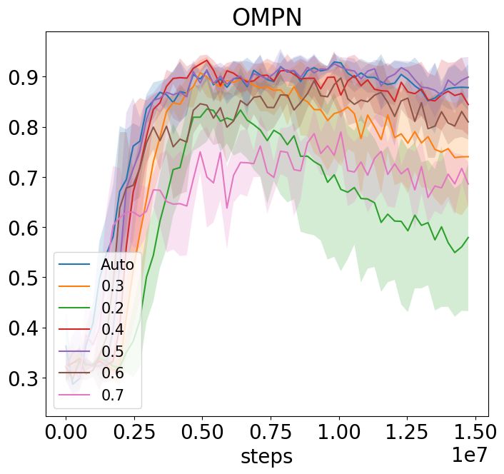
Under review as a conference paper at ICLR 2021

                                             MakeBridge     MakeBridge    MakeBridge    MakeBridge    MakeBridge

             MakeBridge

                                              GetMaterial   GetMaterial   GetMaterial   GetMaterial   BuildBridge
     GetMaterial    BuildBridge

GetGrass     GetWood      GoFactory            GetWood       GetWood      GetGrass      GetGrass      GoFactory

                                  (a)

                                                                             (b)

Figure 1: (a) A simple grid world with the task “make bridge”, which can be decomposed into
multi-level subtask structure. (b) The representation of subtask structure within the agent memory
with horizontal update and vertical expansion at each time step. The black arrow indicates a copy
operation. The expansion position is the memory slot where the vertical expansion starts and is
marked blue.

and BuildBridge. GetM aterial can be further divided into GetGrass and GetW ood. We pro-
vide a sketch on how this subtask structure should be represented inside the agent’s memory during
each time step. The memory would be divided into different levels, corresponding to the subtask
structure. When t = 1, the model just starts with the root task, M akeBridge, and vertically expands
into GetM aterial, which further vertically expands into GetW ood. The vertical expansion corre-
sponds to planning or calling the next level subtasks. The action is produced from the lowest-level
memory. The intermediate GetM aterial is copied for t < 3, but horizontally updated at t = 3,
when GetW ood is finished. The horizontal update can be thought of as an internal update for each
subtask, and the updated GetM aterial vertically expands into a different child GetGrass. The
root task is always copied until GetM aterial is finished at t = 4. As a result, M akeBridge goes
through one horizontal update at t = 5 and then expands into BuildBridge and GoF actory. We
can identify the subtask boundaries from this representation by looking at the change of expansion
position, which is defined to be the memory slot where vertical expansion happens. E.g., from t = 2
to t = 3, the expansion position goes from the lowest level to the middle level, suggesting the com-
pletion of the low-level subtask. From t = 4 to t = 5, the expansion position goes from the lowest
level to the highest level, suggesting the completion of both low-level and mid-level subtasks.
Driven by this intuition, we propose the Ordered Memory Policy Network (OMPN) to support the
subtask hierarchy described in Figure 1. We propose to use a bottom-up recurrence and a top-
down recurrence to implement horizontal update and vertical expansion respectively. Our proposed
memory-update rule further maintains a hierarchy among memories such that the higher-level mem-
ory can store longer-term information like root task information, while the lower-level memory can
store shorter-term information like leaf subtask information. At each time step, the model would
softly decide the expansion position from which to perform vertical expansion based on a differen-
tiable stick-breaking process, so that our model can be trained end-to-end.
We demonstrate the effectiveness of our approach with multi-task behavior cloning. We perform
experiments on a grid-world environment called Craft, as well as a robotic environment called Dial
with a continuous action space. We show that in both environments, OMPN is able to perform task
decomposition in both an unsupervised and weakly supervised manner, comparing favorably with
strong baselines. Meanwhile, OMPN still maintains the similar, if not better, performance on behav-
ior cloning in terms of sample complexity and returns. Our ablation study shows the contribution
of each component in our architecture. Our visualization further confirms that the subtask hierarchy
emerges in our model’s expanding positions.

2     O RDERED M EMORY P OLICY N ETWORK

We describe our policy architecture given the intuition described above. Our model is a recurrent
policy network p(at |st , M t ) where M ∈ Rn×m is a block of n memory while each memory has
dimension m. We use Mi to refer to the ith slot of the memory, so M = [M1 , M2 , ..., Mn ]. The
highest-level memory is Mn while the lowest-level memory is M1 . Each memory can be thought of
as the representation of a subtask. We use the superscript to denote the time step t.

                                                   2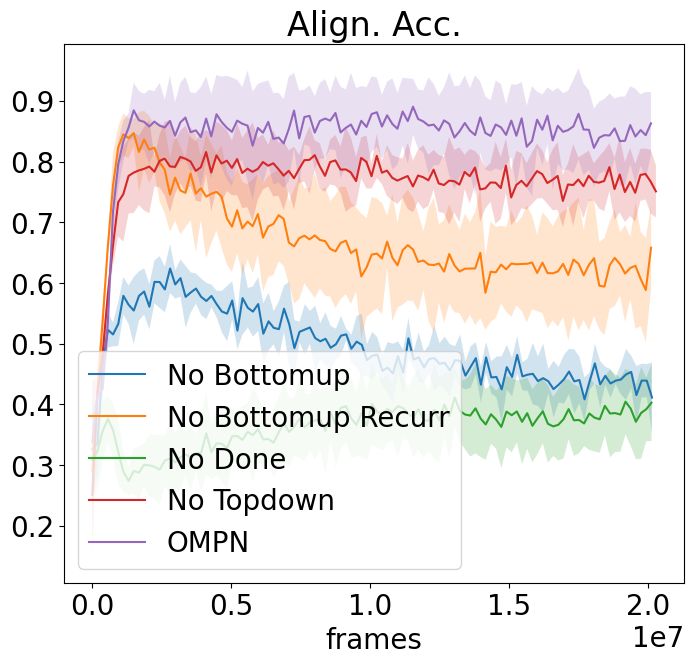
Under review as a conference paper at ICLR 2021

At each time step, our model will first transform the observation st ∈ S to xt ∈ Rm . This can
be achieved by a domain-specific observation encoder. Then we have an ordered-memory module
M t , Ot = OM (xt , M t−1 ) to generate the next memory and the output. The output Ot is sent into
a feed-forward neural net to generate the action distribution.

2.1   O RDERED M EMORY M ODULE

                        Bottom Up
                                                                             Bottom Up

                                                                                                  Top Down

                        (a)                                                              (b)
                           Bottom Up                                                MakeBridge               MakeBridge

                                             Top Down

                                                                                    GetMaterial              BuildBridge

                                                                                     GetGrass                GoFactory

                                                                                          t=4                    t=5

                                       (c)                                                           (d)

Figure 2: Dataflow of how M t−1 will be updated in M t for three memory slots when the expansion
position is at a (a) low, (b) middle, or (c) high position. Blue arrows and red arrows corresponding to
the vertical expansions and horizontal updates. (d) is a snapshot of t = 5 from the grid-world exam-
ple Figure 1b. The subtask-update behavior corresponds to the memory-update when the expansion
position is at the high position.

The ordered memory module first goes through a bottom-up recurrence. This operation implements
the horizontal update and updates each memory with the new observation. We define C t to be the
updated memory:
                                    Cit = F(Ci−1
                                             t
                                                 , xt , Mit−1 )
for i = 1, ..., n where C0t = xt and F is a cell function. Different from our mental diagram, we
make it an recurrent process since the high-level memory might be able to get information from the
updated lower-level memory in addition to the observation. In our experiment we find that such
recurrence will help model perform better than in task decomposition. For each memory, we also
generate a score fit from 0 to 1 with fit = G(xt , Cit , Mit ) for i = 1, ..., n. The score fit can be
interpreted as the probability that subtask i is completed at time t.
In order to properly generate the final expansion position, we would like to insert the inductive bias
that the higher-level subtask is expanded only if the higher-level subtask is not completed while all
the lower-level subtasks are completed, as is shown in Figure 1b. As a result we use a stick-breaking
process as follows:
                                      (           Qi−1
                                  t     (1 − fit ) j=1 fjt 1 < i ≤ n
                                π̂i =
                                        1 − f1t             i=1

Finally we have the expansion position πit = π̂it / π̂ t as a properly normalized distribution over n
                                                   P
memories. We can also define the ending probability as the probability that every subtask is finished.
                                                                 n
                                                                 Y
                                                         t
                                                        πend =         fit                                                 (1)
                                                                 i=1

                                                             3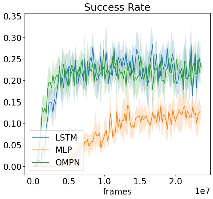
Under review as a conference paper at ICLR 2021

Then we use a top-down recurrence on the memory to implement the vertical expansion. Starting
from M̂nt = 0, we have
                             M̂it = h(π~ti+1 Ci+1
                                              t
                                                  + (1 − π~ti+1 )M̂i+1t
                                                                         , xt ),
where ~πit = j≥i πjt , π~ti = j≤i πjt , and h can be any cell function. Then we update the memory
              P               P
in the following way:
                             M t = M t−1 (1 − ~π t ) + C t π t + M̂ t (1 − π~t )               (2)
where the output is read from the lowest-level memory Ot = M1t . For better understanding purpose,
we show in Figure 2 how M t−1 will be updated into M t with n = 3, when the expansion position
is at a high, middle and low position respectively. The memory higher than the expansion position
will be preserved, while the memory at and lower than the expansion position will be over-written.
We also take the snapshot of t = 5 from our the early example in Figure 1b and show that the
subtask-update behavior corresponds to our memory-update when the expansion position is at the
high position.
Although we show only the discrete case for illustration, the vector π t is actually continuous. As a
result, the whole process is fully differentiable and can be trained end-to-end. More details can be
found in the appendix A.
The memory depths n is a hyper-parameter here. If n is too small, we might not have enough
capacity to cover the underlying structure in the data, If n is too large, we might impose some extra
optimization difficulty. In our experiments we investigate the effect of using different n.

2.2   U NSUPERVISED TASK D ECOMPOSITION WITH B EHAVIOR C LONING

We assume the following setting. We firstly have a training phase to perform behavior cloning on
an unstructured demonstration dataset with state-action pairs. Then during the detection phase, the
user would specify the number of subtasks K for the model to produce the task boundaries.
We firstly describe our training phase. We develop a unique regularization technique which can help
our model learning the underlying hierarchy structure. Suppose we have an action space A. We first
augment this action space with A0 = A ∪ {done}, where done is a special action. Then we can
modify the action distribution accordingly:
                                            t t          t
                                            p(a |s )(1 − πend ) at ∈ A
                            p0 (at |st ) =   t
                                            πend                at = done
Then for each demonstration trajectory τ = {st , at }Tt=1 , we transformed it into τ 0 = τ ∪
{sT +1 , aT +1 = done}, which is essentially telling the model to output done only after the end
of the trajectory. This process can be achieved on both discrete and continuous action space without
                                                                              PT +1
heavy human involvement described in Appendix A. Then we will maximize t=1 log p0 (at |st ) on
  0                            t
τ . We find that including πend into the loss is crucial to prevent our model degenerating into only
using the lowest-level memory, since it provides the signal to raise the expansion position at the end
of the trajectory, benefiting the task decomposition performance. We also justify this in our ablation
study.
Since the expansion position should be high if the low-level subtasks are completed, we can achieve
unsupervised task decomposition by monitoring the behavior of π t . To be specific, we define πavg
                                                                                               t
                                                                                                   =
Pn       t
   i=1 iπi as the expected expansion position. Given πavg , we consider the following methods to
recover the subtask boundaries.

Top-K In this method we choose the time steps of K largest πavg to detect the boundary, where
K is the desired number of sub-tasks given by the user during the detection phase. We find that
this method is suitable for the discrete action space, where there is a very clear boundary between
subtasks.

Thresholding In this method we standardize the πavg into π̂avg from 0 to 1, and then we compute
a Boolean array 1(πavg > thres), where thres is from 0 to 1. We retrieve the subtask boundaries
from the ending time step of each T rue segments. We find this method is suitable for continuous
control settings, where the subtask boundaries are more ambiguous and smoothed out across time
steps. We also design an algorithm to automatically select the threshold in Appendix B.

                                                  4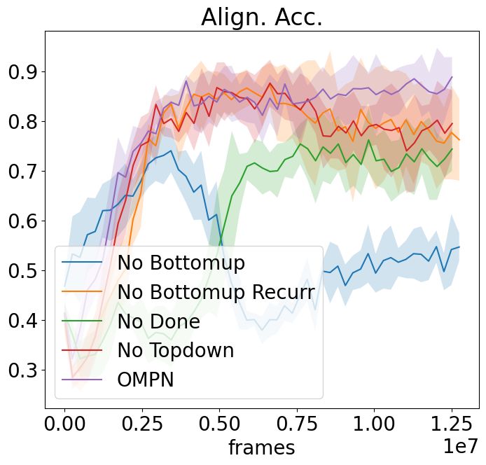
Under review as a conference paper at ICLR 2021

3   R ELATED W ORK
Our work is related to option discovery and hierarchical imitation learning. The existing option
discovery works have focused on building a probabilistic graphical model on the trajectory, with op-
tions as latent variables. DDO (Fox et al., 2017) proposes an iterative EM-like algorithm to discover
multiple level of options from the demonstration. DDO was later applied in the continuous action
space (Krishnan et al., 2017) and program modelling (Fox et al., 2018). Recent works like com-
pILE (Kipf et al., 2019) and VALOR (Achiam et al., 2018) also extend this idea by incorporating
more powerful inference methods like VAE (Kingma & Welling, 2013). Lee (2020) also explore
unsupervise task decompostion via imitation, but their method is not fully end-to-end, requires an
auxiliary self-supervision loss, and does not support multi-level structure. Our work focuses on the
role of neural network inductive bias in discovering re-usable options or subtasks from demonstra-
tion. We do not have an explicit “inference” stage in our training algorithm to infer the option/task
ID from the observations. Instead, this inference ”stage” is implicitly designed into our model ar-
chitecture via the stick-breaking process and expansion position. Based on these considerations, we
choose compILE as the representative baseline for this field of work.
Our work is also related to Hierarchical RL (Vezhnevets et al., 2017; Nachum et al., 2018; Bacon
et al., 2017). These works usually propose an architecture that has a high-level controller to output
a goal, while the low-level architecture takes the goal and outputs the primitive actions. However,
these works mainly deal with the control problem, and do not focus on learning task decomposition
from the demonstration. Recent works (Gupta et al., 2019; Lynch et al., 2020) also include hierarchi-
cal imitation learning stage as a way to pretraining low-level policies before apply Hierarchical RL
for finetuning, however they do not produce the task boundaries and therefore are not comparable to
our works. Moreover, their hierarchical IL algorithm exploits the fact that the goal can be described
as a point in the state space, so that they are able to re-label the ending state of an unstructured
demonstrations as a fake goal to train the goal-conditioned policy. Meanwhile our approach is de-
signed to be general. In addition to the option framework, our work is closely related to Hierarchical
Abstract Machine (HAM) (El Hihi & Bengio, 1996). Our concept of subtask is similar to the finite
state machine (FSM). The horizontal update corresponds to the internal update of the FSM, while
the vertical expansion corresponds to calling the next level of the FSM. Our stick-breaking process
is also a continuous realization of the idea that low-level FSM transfers control back to high-level
FSM at completion.
Recent work (Andreas et al., 2017) introduces the modular policy networks for reinforcement learn-
ing so that it can be used to decompose a complex task into several simple subtasks. In this setting,
the agent is provided a sequence of subtasks, called sketch, at the beginning. Shiarlis et al. (2018)
propose TACO to jointly learn sketch alignment with action sequence, as well as imitating the tra-
jectory. This work can only be applied in the ”weakly supervised” setting, where they have some
information like the sub-task sequence. Nevertheless, we also choose TACO (Shiarlis et al., 2018)
as one of our baselines.
Incorporating varying time-scale for each neuron to capture hierarchy is not a new idea (Chung
et al., 2016; El Hihi & Bengio, 1996; Koutnik et al., 2014). However, these works do not focus on
recovering the structure after training, which makes these methods less interpretable. Shen et al.
(2018) introduce Ordered Neurons and show that they can induce syntactic structure by examin-
ing the hidden states after language modelling. However ONLSTM does not provide mechanism to
achieve the top-down and bottom-up recurrence. Our model is mainly inspired by the Ordered Mem-
ory (Shen et al., 2019). However, unlike previous work our model is a decoder expanding from root
task to subtasks, while the Ordered Memory is an encoder composing constituents into sentences.
Recently Mittal et al. (2020) propose to combine top-down and bottom-up process. However their
main motivation is to handle uncertainty in the sequential prediction and they do not maintain a
hierarchy of memories with different update frequencies.

4   E XPERIMENT
We would like to evaluate whether OMPN is able to jointly learning task decomposition during
behavior cloning. We would like to answer the following questions in our experiments.
    Q1: Can OMPN be applied in both continuous and discrete action space?

                                                  5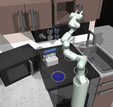
Under review as a conference paper at ICLR 2021

      Q2: Can OMPN be applied in both unsupervised, as well as, weakly supervised setting for task
          decomposition?
      Q3: How much does each component helps the task decomposition?
      Q4: How does the task decomposition performance change with different hyper-parameters,
          e.g., memory dimension m and memory depths n?

4.1     S ETUP AND M ETRICS

For the discrete action space, we use a grid world environment called Craft adapted from Andreas
et al. (2017)1 . At the beginning of each episode, an agent is equipped with a task along with the
sketch, e.g. makecloth = (getgrass, gof actory). The original environment is fully observable.
To further test our model, we make it also support partial observation by providing a self-centric
window. For the continuous action space, we have a robotic setting called Dial (Shiarlis et al., 2018)
where a JACO 6DoF manipulator interact with a large number pad2 . For each episode, the sketch is a
sequence of numbers to be pressed. More details on the demonstration can be found in Appendix E.
We experiment in both unsupervised and weakly supervised settings. For the unsupervised setting,
we did not provide any task information. For the weakly supervised setting, we provide the subtask
sequence, or sketch, in addition to the observation. We use nosketch and sketch to denote these
two settings respectively. We choose compILE to be our unsupervised baseline while TACO to be
our weakly supervised baseline.
We use the ground-truth K to get the best performance of both our models and the baselines. This
setting is consistent with the previous literature (Kipf et al., 2019). The details about task decompo-
sition metric can be found in the appendix C.

4.2     TASK D ECOMPOSITION R ESULTS

                                                            Craft
                                                                                             Dial
                                           Full                           Partial
                                Align Acc     F1(tol=1)        Align Acc       F1(tol=1)   Align Acc
        NoSketch    OMPN         93(1.7)          95(1.2)            84(6)      89(4.6)     87(4.0)
                    compILE      86(1.4)          97(0.8)           54(1.4)     57(4.8)     45(5.2)
                    OMPN         97(1.2)          98(0.9)       78(10.7)        83(8.1)     84(5.7)
        Sketch
                    TACO         90(3.6)             -          66(2.2)            -        98(0.1)

Table 1: Alignment accuracy and F1 scores with tolerance 1 on Craft and Dial. The results are
averaged over five runs, and the number in the parenthesis is the standard deviation.

In this section, we mainly address the question Q1 and Q2. Our main results for task decomposition
in Craft and Dial are in Table 1. In Craft, we use the T opK detection algorithm. Our results show
that OMPN is able to outperform baselines in both unsupervised and weakly-supervised settings
with a higher F1 scores and alignment accuracy. In general, there is a decrease of the performance
for all models when moving from full observations to partial observations. Nevertheless, compared
with the baselines, we find that OMPN suffers less performance drop than the baselines. The F1
score results with different K other than the ground truth is in Table 5 and Table 6.
In Dial, we use the automatic threshold method described in Appendix B. Our results is able to
outperform compILE for the unsupervised setting, but is not better than TACO when the sketch
information is given. In general, our current model does not benefit from the additional sketch
information, and we hypothesize that it is because we use a very trivial way of incorporating sketch
information by simple concatenating it with the observation. A more effective way would be using
attention over the sketch sequence to properly feed the related task information into the model. The
F1 score results with different K other than the ground truth is in Table 8.
   1
       https://github.com/jacobandreas/psketch
   2
       https://github.com/KyriacosShiarli/taco/tree/master/taco/jac

                                                     6
Under review as a conference paper at ICLR 2021

          Factory                                                                   Iron       Grass
          Toolshed
                                                                                   Agent       Wood
          Workbench

Figure 3: Visualization of the learnt expanding positions on Craft. We present π and the action
sequence. The four subtasks are GetW ood, GoT oolshded, GetGrass and GoW orkbench. In the
action sequence, “u” is either picking up/using the object. Each ground truth subtask is highlighted
with an arrow of different colors.

4.3   Q UALITATIVE A NALYSIS

In this section, we provide some visualization of the learnt expanding positions to qualitatively
evaluate whether OMPN can operate with a subtask hierarchy.

                                             9                     3                       3
                           Init                   8
                                                            6

                                     Init

                                        9                   8                      6

Figure 4: Visualization of the learnt expanding positions of Dial domain. The task is to press the
number sequence [9, 8, 6, 3]. We plot the π̂avg . Our threshold selection algorithm produce a upper
bound and and lower bound, and the final threshold is computed as the average. The task boundary
is detected as the last time step of a segment above the final threshold. The frames at the detected
task boundary show that the robot just finishes each subtask.

We firstly visualize the behavior of expanding positions for Craft in Figure 3. We find that at the end
of each subtask, the model learns to switch to a higher expansion position when facing the target
object/place, while within each subtask, the model learns to maintain the lower expansion position.
This is our desired behavior described in Figure 1. What is interesting is that although the ground
truth hierarchy structure might be only two-levels, our model is able to learn multiple level hierarchy
if given some redundant depths. In this example, the model combines the first two subtasks into one
group and the last two subtasks into another group. More results can be found in Appendix F.
In Figure 4, we show the qualitative result in Dial. We find that, instead of having a sharp sub-
task boundary, the boundary between subtasks is more ambiguous with high expanding positions

                                                  7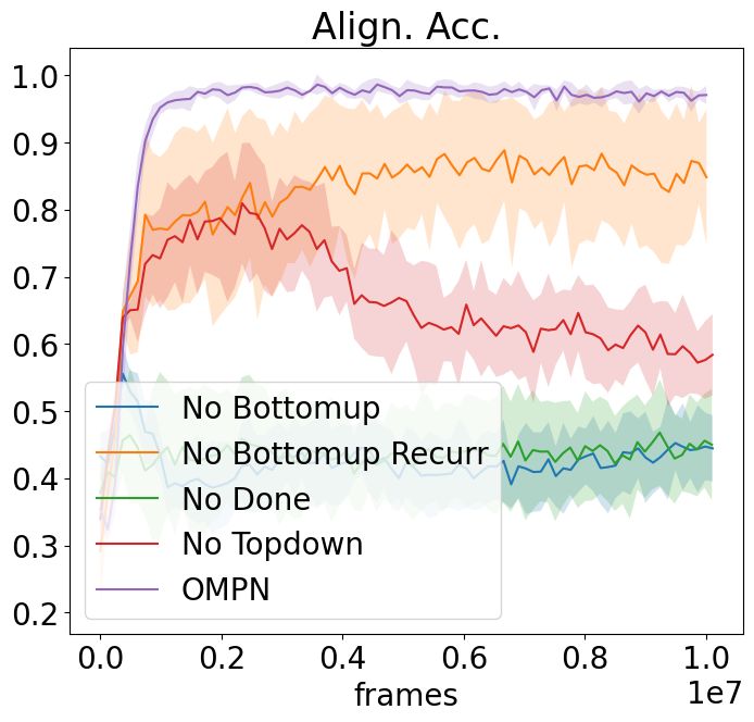
Under review as a conference paper at ICLR 2021

across multiple time steps, and this motivates our design of the threshold algorithm. This happens
because we use the observation to determine the expanding position. In Dial, the state difference
are less significant due to a small time skip and continuous space, so the expanding position near
the boundaries might be high for multiple time steps. Also just like in Craft, the number of subtasks
naturally emerge from the peak patterns. We also provide addition qualitative result on Kitchen
released by Gupta et al. (2019) in Figure 5. More results on Kitchen can be found in Appendix I.

                                 Init                                   D                        D

                                                  A     B      C

                                          Init

                                   A                               B                   C

Figure 5: Visualization of the learnt expanding positions of Kitchen. The subtasks are Microwave,
Bottom Knob, Hinge Cabinet and Slider. We show the upper bound, lower bound and final threshold
produced by our detection algorithm.

4.4     A BLATION S TUDY

  (a) NoSketch + Craft(Full)            (b) NoSketch + Craft(Partial)       (c) NoSketch + Dial

      (d) Sketch + Craft(Full)           (e) Sketch + Craft(Partial)         (f) Sketch + Dial

                  Figure 6: Ablation study for task alignment accuracy for all settings.

                                                       8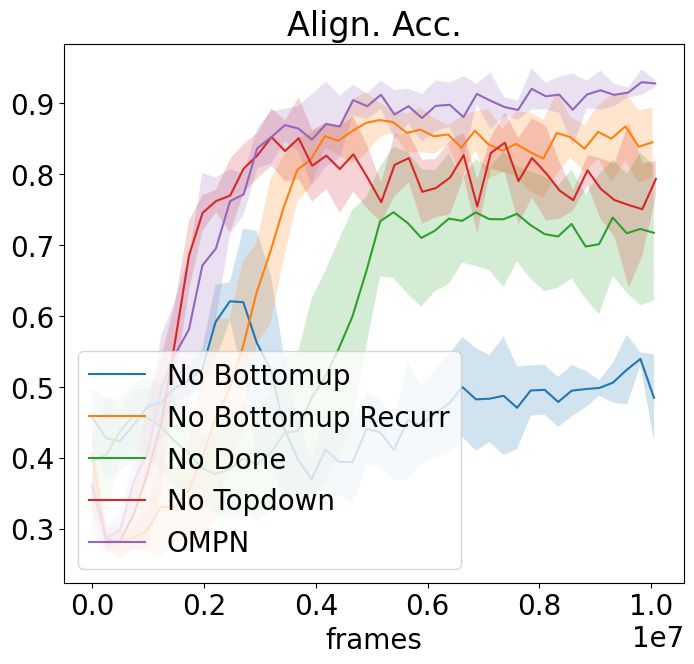
Under review as a conference paper at ICLR 2021

In this section, we aim to answer Q3 and Q4. We perform the ablation study as well as some
hyper-parameter analysis. The results are in Figure 6. We summarize our findings as below:
For No Bottomup and No Topdown, we remove completely either the bottom-up or the top-bottom
process from the model. We find that both hurt the alignment accuracy and removing bottom-up
process hurts more. This is expected since bottom-up recurrence updates the subtasks with the latest
observations before predicting the termination scores, while the top-down process is more related to
outputting actions.
For No Bottomup Recurr, we remove the recurrence in the bottom-up process by making Cit =
F(0, xt , Mit−1 ) so as to preserve the same number of parameters as OMPN. Although this hurts
the alignment accuracy least, the existence of the performance drop confirms our intuition that the
outputs of the lower-level subtasks are beneficial for the higher-level subtasks to predict termination
scores, resulting in better task decomposition.
For No Done, we use the OMPN architecture but remove the πend from the loss. We find that the
model is still able to learn the structure based on the inductive bias to some degree, but the alignment
accuracy is much worse.
We also perform hyper-parameter analysis and see its effect on the task decomposition results in
Appendix H. We find that our task decomposition results is robust to the memory depths n and
memory size m in most cases.

4.5   B EHAVIOR C LONING

We show the behavior cloning results in Figure 7 and the full results are in Figure 10. For Craft,
the sketch information is necessary to make the task solvable, so we don’t see much difference
when there is no sketch information. On the contrary, with full observation and sketch information
(Figure 7a), this setting might be too easy to show the difference since a memory-less MLP can
also achieve almost perfect success rate. As a result, only when the environment moves to a more
challenging but still solvable setting with partial observation (Figure 7b), OMPN outperform LSTM
on the success rate.
For Dial, we find that behaviour cloning alone is not able to solve the task and all of our models
never generate the maximum return due to the exposure bias. This is consistent with the previous
literature on applying behavior cloning to robotics tasks with continuous states (Laskey et al., 2017).
More details can be found in Figure 13.

       (a) Craft Full             (b) Craft Partial                      (c) Dial

Figure 7: The behavior cloning results when sketch information is provided. For Craft, we define
success as the completion of four subtasks. For Dial, the total maximum return is 4.

5     C ONCLUSION
In this work, we investigate the problem of learning the subtask hierarchy from the demonstration
trajectory. We propose a novel Ordered Memory Policy Network (OMPN) that can represent the
subtask structure and leverage it to perform unsupervised task decomposition. Our experiments
show that OMPN learns to recover the ground truth subtask boundary in both unsupervised and
weakly supervised settings with behavior cloning. In the future, we plan to develop a novel control
algorithm based on the inductive bias for faster adaptation to compositional combinations of the
subtasks.

                                                      9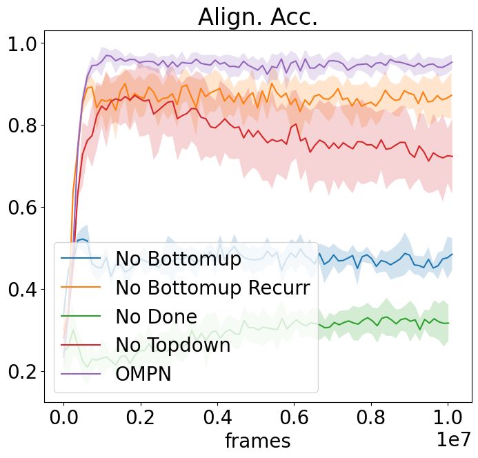
Under review as a conference paper at ICLR 2021

R EFERENCES
Joshua Achiam, Harrison Edwards, Dario Amodei, and Pieter Abbeel. Variational option discovery
  algorithms. arXiv preprint arXiv:1807.10299, 2018. 1, 5

Jacob Andreas, Dan Klein, and Sergey Levine. Modular multitask reinforcement learning with
  policy sketches. In International Conference on Machine Learning, pp. 166–175, 2017. 1, 5, 6

Pierre-Luc Bacon, Jean Harb, and Doina Precup. The option-critic architecture. In Thirty-First AAAI
  Conference on Artificial Intelligence, 2017. 5

Junyoung Chung, Sungjin Ahn, and Yoshua Bengio. Hierarchical multiscale recurrent neural net-
  works. arXiv preprint arXiv:1609.01704, 2016. 5

Salah El Hihi and Yoshua Bengio. Hierarchical recurrent neural networks for long-term dependen-
  cies. In Advances in neural information processing systems, pp. 493–499, 1996. 5

Roy Fox, Sanjay Krishnan, Ion Stoica, and Ken Goldberg. Multi-level discovery of deep options.
  arXiv preprint arXiv:1703.08294, 2017. 1, 5

Roy Fox, Richard Shin, Sanjay Krishnan, Ken Goldberg, Dawn Song, and Ion Stoica. Parametrized
  hierarchical procedures for neural programming. ICLR 2018, 2018. 5

Abhishek Gupta, Vikash Kumar, Corey Lynch, Sergey Levine, and Karol Hausman. Relay policy
  learning: Solving long-horizon tasks via imitation and reinforcement learning. arXiv preprint
  arXiv:1910.11956, 2019. 1, 5, 8, 20

Diederik P Kingma and Max Welling.           Auto-encoding variational bayes.      arXiv preprint
  arXiv:1312.6114, 2013. 5

Thomas Kipf, Yujia Li, Hanjun Dai, Vinicius Zambaldi, Alvaro Sanchez-Gonzalez, Edward Grefen-
  stette, Pushmeet Kohli, and Peter Battaglia. Compile: Compositional imitation learning and
  execution. In International Conference on Machine Learning, pp. 3418–3428. PMLR, 2019. 1,
  5, 6

Jan Koutnik, Klaus Greff, Faustino Gomez, and Juergen Schmidhuber. A clockwork rnn. In Inter-
  national Conference on Machine Learning, pp. 1863–1871, 2014. 5

Sanjay Krishnan, Roy Fox, Ion Stoica, and Ken Goldberg. Ddco: Discovery of deep continuous
  options for robot learning from demonstrations. arXiv preprint arXiv:1710.05421, 2017. 5

Michael Laskey, Jonathan Lee, Roy Fox, Anca Dragan, and Ken Goldberg. Dart: Noise injection
 for robust imitation learning. arXiv preprint arXiv:1703.09327, 2017. 9

Sang-Hyun Lee. Learning compound tasks without task-specific knowledge via imitation and self-
  supervised learning. In International Conference on Machine Learning, 2020. 5

Corey Lynch, Mohi Khansari, Ted Xiao, Vikash Kumar, Jonathan Tompson, Sergey Levine, and
  Pierre Sermanet. Learning latent plans from play. In Conference on Robot Learning, pp. 1113–
  1132. PMLR, 2020. 5

Sarthak Mittal, Alex Lamb, Anirudh Goyal, Vikram Voleti, Murray Shanahan, Guillaume Lajoie,
  Michael Mozer, and Yoshua Bengio. Learning to combine top-down and bottom-up signals in
  recurrent neural networks with attention over modules. arXiv preprint arXiv:2006.16981, 2020.
  5

Ofir Nachum, Shixiang Shane Gu, Honglak Lee, and Sergey Levine. Data-efficient hierarchical
  reinforcement learning. In Advances in Neural Information Processing Systems, pp. 3303–3313,
  2018. 5

Ronald Parr and Stuart J Russell. Reinforcement learning with hierarchies of machines. In Advances
  in neural information processing systems, pp. 1043–1049, 1998. 1

                                                10
Under review as a conference paper at ICLR 2021
Yikang Shen, Shawn Tan, Alessandro Sordoni, and Aaron Courville. Ordered neurons: Integrating
tree structures into recurrent neural networks. In International Conference on Learning Repre-
sentations, 2018. 5
Yikang Shen, Shawn Tan, Arian Hosseini, Zhouhan Lin, Alessandro Sordoni, and Aaron C
Courville. Ordered memory. In Advances in Neural Information Processing Systems, pp. 5037–
5048, 2019. 5, 12
Kyriacos Shiarlis, Markus Wulfmeier, Sasha Salter, Shimon Whiteson, and Ingmar Posner. Taco:
Learning task decomposition via temporal alignment for control. In International Conference on
Machine Learning, pp. 4654–4663, 2018. 1, 5, 6, 13, 15
David Silver, Aja Huang, Chris J Maddison, Arthur Guez, Laurent Sifre, George Van Den Driessche,
Julian Schrittwieser, Ioannis Antonoglou, Veda Panneershelvam, Marc Lanctot, et al. Mastering
the game of go with deep neural networks and tree search. nature, 529(7587):484–489, 2016. 1
Alec Solway, Carlos Diuk, Natalia Córdova, Debbie Yee, Andrew G Barto, Yael Niv, and Matthew M
Botvinick. Optimal behavioral hierarchy. PLOS Comput Biol, 10(8):e1003779, 2014. 1
Richard S Sutton, Doina Precup, and Satinder Singh. Between mdps and semi-mdps: A frame-
work for temporal abstraction in reinforcement learning. Artificial intelligence, 112(1-2):181–
211, 1999. 1
Alexander Sasha Vezhnevets, Simon Osindero, Tom Schaul, Nicolas Heess, Max Jaderberg, David
Silver, and Koray Kavukcuoglu. Feudal networks for hierarchical reinforcement learning. arXiv
preprint arXiv:1703.01161, 2017. 5
Oriol Vinyals, Igor Babuschkin, Wojciech M Czarnecki, Michaël Mathieu, Andrew Dudzik, Juny-
oung Chung, David H Choi, Richard Powell, Timo Ewalds, Petko Georgiev, et al. Grandmaster
level in starcraft ii using multi-agent reinforcement learning. Nature, 575(7782):350–354, 2019.
1
11Under review as a conference paper at ICLR 2021
A OMPN A RCHITECTURE D ETAILS
We use the gated recursive cell function from Shen et al. (2019) in the top-down and bottom up
recurrence. We use a two-layer MLP to compute the score fi for the stick-breaking process. For the
initial memory M 0 , we send the environment information into the highest slot while keep the rest
of the slots to be zeros. If unsupervised setting, then the every slot is initialized as zero. At the first
time step, we also skip the bottom-up process and hard code π 1 such that the memory expands from
the highest level. This is used to make sure that at first time step, we could propagate our memory
with the expanded subtasks from root task. In our experiment, our cell functions does not share the
parameters. We find that to be better than shared-parameter.
We set the number of slots to be 3 in both Craft and Dial, and each memory has dimension 128.
We use Adam optimizer to train our model with β1 = 0.9, β2 = 0.999. The learning rate is 0.001
in Craft and 0.0005 in Dial. We set the length of BPTT to be 64 in both experiments. We clip the
gradients with L2 norm 0.2. The observation has dimension 1076 in Craft and 39 in Dial. We use
a linear layer to encode the observation. After reading the output Ot , we concatenate it with the
observation xt and send them to a linear layer to produce the action.
In section 2, we describe that we augment the action space into A ∪ {done} and we append the
trajectory τ = {st , at }Tt=1 with one last step, which is τ ∪ {st+1 , done}. This can be easily done if
the data is generated by letting an expert agent interact with the environment as in Algorithm 1. If
you do not have the luxury of environment interaction, then you can simply let sT +1 = sT , aT +1 =
done. We find that augmenting the trajectory in this way does not change the performance in our
Dial experiment, since the task boundary is smoothed out across time steps for continuous action
space, but it hurts the performance for Craft, since the final action of craft is usually U SE, which
can change the state a lot.
Algorithm 1: Data Collection with Gym API
env = gym.make(name)
done = False
obs = env.reset()
traj = []
repeat
action = bot.act(obs)
nextobs, reward, done = env.step(action)
traj.append((obs, action, reward))
obs = nextobs
until done is True;
traj.append((obs, done action))
B T HRESHOLDING A LGORITHM
We here provide the peseudo-code for our threshold algorithm. Algorithm 2, we detect boundary by
recording the time steps which goes from above to below the given threshold. We return the final K
time steps where K is given. We assume the last subtask ends when the episode ends.
We design Algorithm 3 to automatically select the threshold. Our intuition is that, the optimal
threshold should pass through K peaks, where K is the provided by the users. As a result, we pick
the highest peak and the lowest valley as the upper bound and lower bound for the threshold, and we
return the final threshold as the middle of these two.
C TASK D ECOMPOSITION M ETRIC
C.1 F1 S CORES WITH T OLERANCE
For each trajectory, we are given a set of ground truth task boundary gt of length L which is the
number of subtasks. The algorithm also produce L task boundary predictions. This can be done in
12Under review as a conference paper at ICLR 2021
Algorithm 2: Get boundary from a given threshold
Data: Standardized average expanding positions πavg
ˆ with length L, the number of subtasks
K, and a threshold T
Result: A list of K split points.
preds = []
prev = F alse
for t in range(L) do
curr = [πavgˆ [t] > T ]
if prev == curr then
continue
else
if prev and not curr then
preds.append(t − 1)
prev = curr
preds.append(L − 1)
Return preds[:: −1][: K][:: −1]
Algorithm 3: Automatic threshold selection
Data: Standardized average expanding positions πavg ˆ with length L
Result: A final threshold T
diff = πavg
ˆ [1:] - πavg
ˆ [:-1]
upid = [i for i in range(1, len(diff)) if diff[i] < 0 and diff[i-1] > 0]
lowid = [i for i in range(1, len(diff)) if diff[i] > 0 and diff[i - 1] < 0]
upval = πavg
ˆ [upid]
lowval = πavg
ˆ [lowid]
upper = upval.max()
lower = lowval.min()
final = (upper + lower) / 2
Return final
OMPN by setting the correct K in topK boundary detection. For compILE, we set the number of
segments to be equal to N . Nevertheless, our definition of F1 can be extended to arbitaray number
of predictions.
P
i,j match(predsi , gtj , tol)
precision =
#predictions)
P
i,j match(gti , predsj , tol)
precision =
#ground truth
where the match is defined as
match(x, y, tol) = [y − tol ≤ x ≤ y + tol]
where [] is the Iverson bracket. The tolerance
C.2 TASK A LIGNMENT ACCURACY
This metric is taken from Shiarlis et al. (2018). Suppose we have a sketch of 4 subtasks b =
t
[b1, b2, b3, b4] and we have the ground truth assignment ξtrue = {ξtrue }Tt=1 . Similar we have the
predicted alignment ξpred . The alignment accuracy is simply
X
t t
[ξpred == ξtrue ]
t
For OMPN and compILE, we obtain the task boundary first and construct the alignment as a result.
For TACO, we follow the original paper to obtain the alignment.
13Under review as a conference paper at ICLR 2021
D BASELINE
D.1 COMP ILE D ETAILS
latent [concrete, gaussian]
prior [0.3, 0.5,0.7]
kl b [0.05, 0.1, 0.2]
kl z [0.05, 0.1, 0.2]
Table 2: compILE hyperparameter search.
Our implementation of compILE is taken from the author github3 . However, their released code only
work for a toy digit sequence example. As a result we modify the encoder and decoder respectively
for our environments. During our experiment, we perform the following hyper-parameter sweep on
the baseline in Table 2. Although the authors use latent to be concrete during their paper, we find
that gaussian perform better in our case. We find that Gaussian with prior = 0.5 performs the best
in Craft. For Dial, these configurations perform equally bad.
We show the task alignments of compILE for Craft in Figure 8. It seems that compILE learn the task
boundary one-off. However, since the subtask ground truth can be ad hoc, this brings the question
how should we decide whether our model is learning structure that makes sense or not? Further
investigation in building a better benchmark/metric is required.
Figure 8: Task alignment results of compILE on Craft.
D.2 TACO D ETAILS
dropout [0.2, 0.4, 0.6, 0.8]
decay [0.2, 0.4, 0.6, 0.8]
Table 3: TACO hyperparameter search.
We use the implementation from author github4 and modifiy it into pytorch. Although the author
also conduct experiment on Craft and Dial, they did not release the demonstration dataset they use.
As a result, we cannot directly use their numbers from the paper. We also apply dropout on the
prediction of ST OP and apply a linear decaying schedule during training. The hyperparameter
search is in table 3. We find the best hyperparameter to be 0.4, 0.4 for Craft. For Dial, the result is
not sensitive to the hyperparameters.
3
https://github.com/tkipf/compile
4
https://github.com/KyriacosShiarli/taco
14Under review as a conference paper at ICLR 2021
E D EMONSTRATION G ENERATION
We use a rule-based agent to generate the demonstration for both Craft and Dial. For Craft, we train
on 500 episodes each on M akeAxe, M akeShears and M akeBed. Each of these task is further
composed of four subtasks. For Dial, we generate 1400 trajectories for imitation learning with each
sketch being 4 digits.
For Craft with full observations, we design a shortest path solver to go to the target location of each
subtask. For Craft with partial observation, we maintain an internal memory about the currently seen
map. If the target object for the current subtask is not seen on the internal memory, we perform a left-
to-right, down-to-top exploration until the target object appears inside the memory. Once the target
object is seen, it defaults to the behavior in full observations. For Dial, we use the hand-designed
controller in Shiarlis et al. (2018) to generate the demonstration.
F C RAFT
We train our models on M akeBed, M akeAxe, and M akeShears. The detail of their task decom-
position is in Table 4. We show the behavior cloning results for all settings in Figure 10. We display
more visuzliation of task decomposition results from OMPN in Figure 9.
makebed get wood, make at toolshed, get grass, make at workbench
makeaxe get wood, make at workbench, get iron, make at toolshed
makeshears get wood, make at workbench, get iron, make at workbench
Table 4: Details of training tasks decomposition.
Figure 9: More results on π in Craft. The model is able to robustly switch to a higher expanding
position at the end of subtasks. The model will also sometimes discover multi-level hierarchy.
We show the results of task decomposition when the given K is different in table 5 and table 6. We
find that when you increase the K, the recall increases while the precision decreases.
15Under review as a conference paper at ICLR 2021
(a) Full + NoSketch (b) Full + Sketch (c) Partial + NoSketch (d) Partial + Sketch
Figure 10: Behavior Cloning for Craft.
Full NoSketch Full Sketch
F1(tol=1) Pre(tol=1) Rec(tol=1) F1(tol=1) Pre(tol=1) Rec(tol=1)
K=2 62(2.4) 93(3.7) 47(1.8) 62(2.4) 93(3.4) 46(1.8)
K=3 81(2) 95(2.4) 71(1.8) 81(2.2) 95(2.3) 71(2.0)
K=4 95(1.2) 95(1.8) 95(1.8) 98(0.9) 98(1.6) 97(2.1)
K=5 92(1.6) 87(2.8) 99(0.5) 93(6.4) 87(1.1) 99(0.5)
K=6 88(2.9) 78(3.9) 100(0) 88(0.6) 79(0.9) 99(0.2)
Table 5: Parsing results for full observations with different K
Parital NoSketch Partial Sketch
F1(tol=1) Pre(tol=1) Rec(tol=1) F1(tol=1) Pre(tol=1) Rec(tol=1)
K=2 64(1.8) 96(2.7) 48(1.4) 57(3.7) 88(5.6) 43(2.8)
K=3 83(1.9) 96(1.9) 72(1.9) 74(3.9) 88(4.6) 64(3.5)
K=4 89(4.6) 97(1.6) 82(2.7) 83(8.1) 88(4.4) 80(4.6)
K=5 93(0.8) 90(1.9) 96(2.7) 89(3.2) 85(3.7) 94(3.8)
K=6 90(1.9) 85(1.7) 98(2.3) 87(2.1) 813.4) 97(2.3)
Table 6: Parsing results for partial observations with different K
16Under review as a conference paper at ICLR 2021
G D IAL
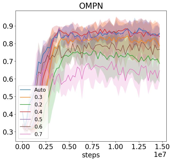
We show in Table 7 the task alignment result for different thresholds. We can see that optimal
fixed threshold is around 0.4 or 0.5 for Dial, and our threshold selection algorithm could produce
competitive results. We demonstrate more expanding positions in Figure 11. We also show the
failure cases, where our selected threshold fails to recover the skill boundary. Nevertheless, we can
see that the peak pattern exists. We show the task alignment curves for different thresholds as well
as the auto-selected threshold in Figure 12.
Align. Acc. at different threshold
0.2 0.3 0.4 0.5 0.6 0.7 Auto
OMPN + noenv 57(12.8) 76(9.5) 87(5.7) 89(1.4) 81(5.7) 70(9.7) 87(4)
OMPN + sketch 71(11.6) 81(10.6) 85(7.4) 84(6.6) 76(7.7) 60(6.4) 84(5.7)
Table 7: Task alignment accuracy for different threshold in Dial. The result for automatic threshold
selection is in the last column.
Figure 11: More task decomposition visualization in Dial. Our algorithm recovers the skill boundary
for the first four trajectories but fails in the last two. Nevertheless, one can see that our model still
display the peak patterns for each subtask, and a more advanced thresholding method could be
designed to recover the skill boundaries.
(a) Dial + NoSketch (b) Dial + Sketch
Figure 12: The learning curves of task alignment accuracy for different thresholds as well as the
automatically selected one.
17Under review as a conference paper at ICLR 2021
The behavior cloning results are in Figure 13.
(a) Dial + NoSketch (b) Dial + Sketch
Figure 13: The behavior cloning results in Dial domain.
We show the task decomposition results when the K is mis-specified in Table 8.
NoSketch Sketch
f1(tol=1) rec(tol=1) pre(tol=1) f1(tol=1) rec(tol=1) pre(tol=1)
K =2 59(2.9) 45(2.1) 90(4.4) 58(1.4) 44(1.1) 88(2.1)
K =3 73(5.5)) 63(5.1) 85(6.2) 72(3.8) 63(3.4) 84(4.5)
K =4 84(7.1) 81(7.1) 84(6.9) 81(4.8) 81(4.6) 82(5.1)
K =5 86(5.1) 91(3.6) 83(6.3) 83(5.2) 86(5.4) 82(5.3)
K =6 87(4.2) 93(1.5) 82(6.2) 84(5.2) 88(5.5) 81(5.2)
K =7 87(4.1) 93(1.4) 82(6.4) 84(5.2) 89(6) 81(5.2)
K =8 86(4.1) 93(1.6) 82(6.6) 84(5.2) 90(6..1) 81(5.1)
Table 8: F1 score, recall and precision with tolerance 1 computed at different k.
18Under review as a conference paper at ICLR 2021
H H YPERPARAMETER A NALYSIS
Craft Full Craft Partial Dial
NoSketch Sketch NoSketch Sketch NoSketch Sketch
n = 3, m = 64 93(1.7) 97(1.2) 84(6) 78(10.7) 87(4) 84(5.7)
n = 2, m = 64 96(1.4) 96(1.4) 87(3.3) 77(1.2) 88(3.2) 82(5.7)
n = 4, m = 64 96(0.6) 96(2.5)) 88(3.1) 73(6.2) 86(9.8) 82(10)
n = 3, m = 32 92(4.2) 91(10.3) 88(6) 74(5.5) 88(4.9) 83(3.7)
n = 3, m = 128 96(1.5) 97(1.2) 86(3) 75(5.7) 87(2.4) 83(6.2)
Table 9: Task alignments accuracy for different memory dimension m and depths n. The default
setting is on the first row. The next two rows change the depths, while the last two rows change the
memory dimension. The number in the parenthesis is the standard deviation.
We discuss the effect of hyper-parameters on the task decomposition results. We summarize the
results in Table 9. We show the detailed alignment accuracy curves for Craft in Figure 14 and for
Dial in Figure 15.
(a) Full + NoSketch (b) Full + Sketch (c) Partial + NoSketch (d) Partial + Sketch
(e) Full + NoSketch (f) Full + Sketch (g) Partial + NoSketch (h) Partial + Sketch
Figure 14: Task alignment accuracy with varying hyperparameters in Craft. We change the depths
in the first row and memory size in the second row.
(a) Dial + NoSketch (b) Dial + NoSketch (c) Dial + Sketch (d) Dial + Sketch
Figure 15: Task alignment accuracy in Dial. In (a) and (c) we change the depths while in (b) and (d)
we change the memory size.
19Under review as a conference paper at ICLR 2021
I Q UALITATIVE R ESULTS ON K ITCHEN
We display the qualitative results for Kitchen. We use the demonstration released by Gupta et al.
(2019). Since they do not provide ground truth task boundaries, we provide the qualitative results.
We use a hidden size of 64 and the memory depths of 2. We set the learning rate to be 0.0001 with
Adam and the BPTT length to be 150. The input dimension is 60 and action dim is 9. We train our
model in the unsupervised (NoSketch) setting. We show the visualization of our expanding position,
in a similar fashion of the Dial domain, in Figure 16 and Figure 17. We show the visualizations for
other trajectories in Figure 18
Init D D
A B C
Init
A B C
Figure 16: Visualization of the learnt expanding positions of Kitchen. The subtasks are Microwave,
Bottom Knob, Hinge Cabinet and Slider.
D
Init D
A B C
Init
A B C
Figure 17: Visualization of the learnt expanding positions of Kitchen. The subtasks are Kettle,
Bottom Knob, Hinge Cabinet and Slider.
20Under review as a conference paper at ICLR 2021
Figure 18: More task decomposition visualization in Kitchen. Our algorithm seems to recover the
skill boundary for the first four trajectories but fails in the last two. Nevertheless, one can see that
our model still display the peak patterns for each subtask, and a more advanced post-processing
thresholding method might be able to recover the task boundary.
21You can also read