Cyanobacteria net community production in the Baltic Sea as inferred from profiling pCO2 measurements
←
→
Page content transcription
If your browser does not render page correctly, please read the page content below
Biogeosciences, 18, 4889–4917, 2021
https://doi.org/10.5194/bg-18-4889-2021
© Author(s) 2021. This work is distributed under
the Creative Commons Attribution 4.0 License.

Cyanobacteria net community production in the Baltic Sea as
inferred from profiling pCO2 measurements
Jens Daniel Müller1,2 , Bernd Schneider1 , Ulf Gräwe3 , Peer Fietzek4 , Marcus Bo Wallin5,6 , Anna Rutgersson5 ,
Norbert Wasmund7 , Siegfried Krüger3 , and Gregor Rehder1
1 Department of Marine Chemistry, Leibniz Institute for Baltic Sea Research Warnemünde, Rostock, Germany
2 Environmental Physics, Institute of Biogeochemistry and Pollutant Dynamics, ETH Zurich, Zurich, Switzerland
3 Department of Physical Oceanography and Instrumentation, Leibniz Institute for Baltic Sea Research Warnemünde,

Rostock, Germany
4 Kongsberg Maritime Germany GmbH, Hamburg, Germany
5 Department of Earth Sciences, Uppsala University, Uppsala, Sweden
6 Department of Aquatic Sciences and Assessment, Swedish University of Agricultural Sciences, Uppsala, Sweden
7 Department of Biological Oceanography, Leibniz Institute for Baltic Sea Research Warnemünde, Rostock, Germany

Correspondence: Jens Daniel Müller (jensdaniel.mueller@usys.ethz.ch)

Received: 21 February 2021 – Discussion started: 1 March 2021
Revised: 7 July 2021 – Accepted: 12 July 2021 – Published: 7 September 2021

Abstract. Organic matter production by cyanobacteria              teristics in common with blooms in previous years. In par-
blooms is a major environmental concern for the Baltic Sea,       ticular, it lasted for about 3 weeks, caused a CT∗ drawdown
as it promotes the spread of anoxic zones. Partial pressure of    of 90 µmol kg−1 , and was accompanied by a sea surface tem-
carbon dioxide (pCO2 ) measurements carried out on Ships          perature increase of 10 ◦ C. The novel finding of this study
of Opportunity (SOOP) since 2003 have proven to be a pow-         is the vertical extension of the CT∗ drawdown up to the com-
erful tool to resolve the carbon dynamics of the blooms in        pensation depth located at around 12 m. Integration of the CT∗
space and time. However, SOOP measurements lack the pos-          drawdown across this depth and correction for vertical fluxes
sibility to directly constrain depth-integrated net community     leads to an NCP best guess of ∼ 1.2 mol m−2 over the pro-
production (NCP) in moles of carbon per surface area due          ductive period.
to their restriction to the sea surface. This study tackles the      Addressing goal (2), we combined modelled hydrograph-
knowledge gap through (1) providing an NCP best guess for         ical profiles with surface pCO2 observations recorded by
an individual cyanobacteria bloom based on repeated profil-       SOOP Finnmaid within the study area. Introducing the tem-
ing measurements of pCO2 and (2) establishing an algorithm        perature penetration depth (TPD) as a new parameter to in-
to accurately reconstruct depth-integrated NCP from surface       tegrate SOOP observations across depth, we achieve an NCP
pCO2 observations in combination with modelled tempera-           reconstruction that agrees to the best guess within 10 %,
ture profiles.                                                    which is considerably better than the reconstruction based
   Goal (1) was achieved by deploying state-of-the-art sen-       on a classical mixed-layer depth constraint.
sor technology from a small-scale sailing vessel. The low-           Applying the TPD approach to almost 2 decades of surface
cost and flexible platform enabled observations covering an       pCO2 observations available for the Baltic Sea bears the po-
entire bloom event that occurred in July–August 2018 in the       tential to provide new insights into the control and long-term
Eastern Gotland Sea. For the biogeochemical interpretation,       trends of cyanobacteria NCP. This understanding is key for
recorded pCO2 profiles were converted to CT∗ , which is the       an effective design and monitoring of conservation measures
dissolved inorganic carbon concentration normalised to alka-      aiming at a Good Environmental Status of the Baltic Sea.
linity. We found that the investigated bloom event was dom-
inated by Nodularia and had many biogeochemical charac-

Published by Copernicus Publications on behalf of the European Geosciences Union.
4890                                                                J. D. Müller et al.: Cyanobacteria NCP in the Baltic Sea

1     Introduction                                                 and mechanistic understanding of organic matter production
                                                                   is key to understand, predict, and eventually counteract the
1.1    Net community production (NCP) in marine                    expansion of the anoxic areas. Such measures to reduce eu-
       ecosystems                                                  trophication and deep water anoxia actually represent a core
                                                                   component of the EU Marine Strategy Framework Directive
Net community production (NCP) of organic matter triggers          (MSFD), which is implemented as the HELCOM Baltic Sea
many biogeochemical processes that control the functioning         Action Plan (BSAP) and aims at a Good Environmental Sta-
and state of marine ecosystems. Globally relevant examples         tus (GES) of the Baltic Sea.
are the biological carbon pump (Henson et al., 2011; Sanders
et al., 2014) and the establishment of oxygen minimum zones        1.3   Cyanobacteria blooms
(Gilly et al., 2013; Oschlies et al., 2018). In this biogeochem-
ical context, we define NCP as the net amount of carbon fixed      The annual cycle of organic matter production in the Central
in organic matter (gross production minus respiration) that is     Baltic Sea can be broadly divided into two phases (Schneider
produced in a defined water volume over a defined period.          and Müller, 2018). The first production phase is the spring
This definition implies that the choice of an integration depth    bloom, which is controlled by the availability of nitrate and
is a critical component of any NCP estimate. Traditionally,        shifted from being dominated by diatoms to dinoflagellates
NCP is constrained to the depth of the euphotic zone, the          in the late 1980s (Wasmund et al., 2017; Spilling et al., 2018).
compensation depth at which gross production equals res-           After a so-called blue water period with close-to-zero NCP
piration, or the mixed-layer depth (Sarmiento and Gruber,          rates, the second production phase consists of midsummer
2006). Of those approaches, only the integration to the com-       blooms dominated by nitrogen-fixing cyanobacteria that de-
pensation depth is directly linked to the vertical distribution    velop in most years depending on meteorological conditions.
of carbon fixation and remineralisation and therefore quanti-      Although cyanobacteria NCP is yet poorly constrained, its
fies the amount of formed organic matter that can potentially      relative contribution to the annual NCP in the Eastern Got-
be exported. The reliable quantification of this potential ex-     land Sea in 2009 was estimated on the order of 40 % (Schnei-
port is a prerequisite to understand subsequent biogeochem-        der and Müller, 2018; Schneider et al., 2014), though the
ical transformation of the organic matter and its imprint on       uncertainty of this estimate is high. This preliminary esti-
environmental conditions in any aquatic system.                    mate further needs to be interpreted with care as cyanobacte-
                                                                   ria NCP varies significantly between years and regions. The
1.2    Baltic Sea                                                  blooming of cyanobacteria is limited to the months of June
                                                                   to August (Kownacka et al., 2020) and represents a common
On a regional scale, NCP quantification is of particular im-       feature of the Baltic Sea ecosystem at least since the 1960s
portance to study deoxygenation of stratified water bodies         (Finni et al., 2001). The blooms are a major public concern,
caused by the remineralisation of organic matter that was ex-      because they produce toxins and form thick surface scums,
ported across a permanent pycnocline. This hydrographical          lowering the recreational value of the Baltic Sea. From a bio-
situation is typically encountered in semi-enclosed, silled es-    geochemical perspective, the ability to fix nitrogen makes
tuaries such as the Baltic Sea. The deep basins of the Baltic      cyanobacteria independent from nitrate and aggravates the
Sea receive substantial amounts of oxygenated, salty wa-           eutrophication state of the Baltic Sea. Whether their growth
ter from the North Sea only during occasional major inflow         is limited by the availability of phosphate remains an ongo-
events. Between inflow events, those water masses can stag-        ing debate (Nausch et al., 2012), although the highly variable
nate for more than a decade below the permanent halocline          C : P ratio of their biomass (Nausch et al., 2009) indicates
(Mohrholz et al., 2015), which is located at around 60 m wa-       phenotypic plasticity. Other ongoing debates in the field of
ter depth in the Central Baltic Sea. The export of organic         cyanobacteria research address the fate of the produced or-
matter into the deep waters is considered the ultimate cause       ganic matter and its transfer into the food web (Karlson et al.,
for the expansion of anoxic areas in the Baltic Sea, which are     2015), the intensification of cyanobacteria blooms through
today among the largest anthropogenically induced anoxic           positive feedback loops between organic matter production,
areas in the world (Carstensen et al., 2014). Although the ac-     deep water anoxia, and the release of phosphate from anoxic
tual oxygenation state of the deep basins of the Baltic Sea        sediments (Vahtera et al., 2007), as well as their response to
is modulated by the frequency and strength of inflow events        ongoing changes in salinity, temperature, and the partial pres-
(Mohrholz et al., 2015; Neumann et al., 2017) and the bio-         sure of carbon dioxide, pCO2 (Olofsson et al., 2019, 2020).
geochemical properties of the inflowing waters (Meier et al.,      The limited understanding of the factors that control the
2018), the long-term expansion of the anoxic water body            blooms hinders the reliable prediction of the future state of
was primarily attributed to increased nutrient inputs from         the Baltic Sea and therefore the prioritisation of conservation
land (Jokinen et al., 2018; Meier et al., 2019; Carstensen         measures (Elmgren, 2001). In particular, it remains challeng-
et al., 2014; Mohrholz, 2018) that fuelled the organic mat-        ing to disentangle how expected trends – including warming,
ter production in surface waters. Therefore, a quantitative        reduced nutrient loads, and increasing pCO2 – might im-

Biogeosciences, 18, 4889–4917, 2021                                                   https://doi.org/10.5194/bg-18-4889-2021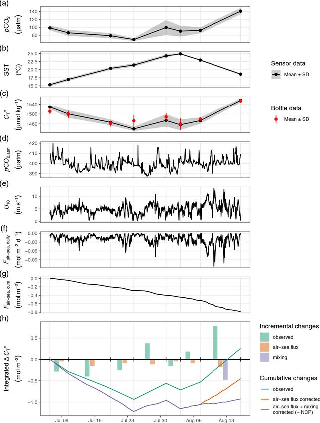
J. D. Müller et al.: Cyanobacteria NCP in the Baltic Sea                                                                   4891

pact cyanobacteria growth (Meier et al., 2019; Saraiva et al.,    pCO2 measurements on the Ship of Opportunity (SOOP)
2019). A long-term hindcast of cyanobacteria NCP and the          Finnmaid played a pivotal role. Those measurements were
attribution of its strength to prevailing environmental condi-    started in 2003, and it was demonstrated that highly accurate
tions in particular years could improve our understanding of      time series of changes (not absolute values) in CT can be de-
controlling factors and facilitate more reliable predictions of   rived from pCO2 observations (Schneider et al., 2006). The
the blooms. However, such a hindcast of cyanobacteria NCP         conversion from pCO2 to CT relies on a fixed alkalinity (AT )
was so far impossible due to missing vertically resolved ob-      estimate and is applicable under the condition that internal
servations that would allow the constraint of their organic       sinks and sources of AT can be excluded, which is the case
matter production.                                                in the Baltic Sea due to the absence of calcifying plankton
                                                                  (Tyrrell et al., 2008). The derived parameter is comparable
1.4   Quantification of NCP                                       to directly measured CT normalised to AT and in the follow-
                                                                  ing referred to as CT∗ . For several years of SOOP observa-
Striving for a better understanding of the ecosystem impact       tions, it was shown that the CT∗ drawdown during midsummer
of cyanobacteria blooms, the accurate quantification of pro-      cyanobacteria blooms occurs in pulses of days to weeks, pri-
duced organic matter is key. In this regard, NCP could in         marily during calm, sunny days. Further, it was found that the
principle be quantified directly as an increase in particulate    CT∗ drawdown correlates well with the co-occurring increase
organic carbon (POC). However, POC measurements would             in sea surface temperature (SST), rather than with absolute
not detect the amount of organic matter that was exported         SST. This relationship was attributed to a common driver,
between observations (Wasmund et al., 2005) and also fail         which is the light dose received by the water mass under con-
to achieve the required spatio-temporal resolution due to a       sideration (Schneider and Müller, 2018).
low degree of automation. As an alternative, it is possible          Despite the successful investigation of cyanobacteria
to quantify NCP through the drawdown of dissolved inor-           blooms through SOOP pCO2 observations, providing a
ganic carbon (CT ) from the water column (Schneider et al.,       depth-integrated estimate of NCP in units of moles carbon
2003). From a biogeochemical perspective, the determina-          fixed per surface area remains challenging due to the restric-
tion of NCP in terms of carbon is ideal, because carbon is        tion of SOOP observations to surface waters. Previous stud-
the major component of organic matter and directly related        ies aiming at a depth-integrated NCP estimate either sim-
to the amount of oxygen (O2 ) that is consumed during rem-        ply assumed that the CT∗ drawdown reached as far down as
ineralisation. In principle, NCP could also be estimated from     the water inlet of the measurement system (Schneider and
O2 time series. However, the equilibrium reactions of carbon      Müller, 2018) or relied on a modelled mixed-layer depth
dioxide (CO2 ) in seawater result in slower re-equilibration      for the vertical integration of surface observations (Schnei-
of CO2 with the atmosphere compared to O2 (Wanninkhof,            der et al., 2014). However, in the absence of any vertically
2014). This results in substantially longer preservation of the   resolved measurements, neither approach could be validated.
CT signal and thus a lower uncertainty contribution of re-        Likewise, remote sensing approaches were capable to resolve
quired air–sea CO2 flux corrections, making CT the preferred      the spatial coverage of the blooms (Hansson and Hakansson,
tracer for NCP. During the Baltic Sea spring bloom, the trac-     2007; Kahru and Elmgren, 2014) but failed to detect their
ing of nutrient drawdown is a meaningful alternative to quan-     vertical extent (Kutser et al., 2008) and quantify NCP. Fi-
tify NCP and convincingly leads to comparable results to the      nally, regular research vessel cruises allowed for the determi-
CT approach (Wasmund et al., 2005). However, time series          nation of a full suite of biogeochemical parameters from dis-
of nutrient drawdown do not allow for determining NCP of          crete water samples and even the experimental determination
algae blooms dominated by nitrogen-fixing organisms and           of carbon fixation rates through 14 C incubations (Wasmund
those with highly variable C : P ratios. As both characteris-     et al., 2001, 2005). Such incubation experiments can provide
tics are typical for Baltic Sea cyanobacteria blooms (Nausch      valuable information about instantaneous rates of NCP, but
et al., 2009), the well-established CT approach remains the       – in contrast to time series observations such as obtained
favourable method to determine midsummer NCP in this re-          by SOOP measurements – do not allow the integration of
gion. However, it should be noted that NCP estimates de-          observed changes over time and constrain budgets of bio-
rived from this approach include the formation of POC and         geochemical transformations. This integration over time re-
dissolved organic carbon (DOC). The produced DOC con-             quires several weeks of repeated observations to resolve the
tributes ∼ 20 % to NCP (Hansell and Carlson, 1998; Schnei-        progression of entire bloom events, ideally covering a station
der and Kuss, 2004) and is not likely to be vertically ex-        network to average bloom patchiness.
ported.
                                                                  1.6   This study
1.5   Previous studies

Among previous attempts to trace and quantify the or-             This study builds upon the previous success to determine
ganic matter production of cyanobacteria blooms, automated        NCP based on pCO2 time series but extends the approach

https://doi.org/10.5194/bg-18-4889-2021                                                  Biogeosciences, 18, 4889–4917, 2021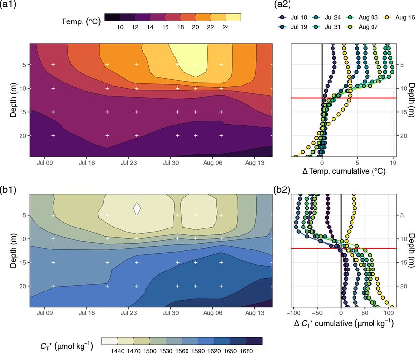
4892                                                                J. D. Müller et al.: Cyanobacteria NCP in the Baltic Sea

to vertically resolved observations for the first time. The pri-   2.2     Field sampling campaign
mary goals of this study are to
                                                                   2.2.1    CTD measurements
    1. provide a best guess for the depth-integrated NCP of an
       individual cyanobacteria bloom based on the full suite
                                                                   CTD measurements were performed with a SBE 16 SeaCAT
       of depth-resolved in situ measurements and
                                                                   instrument (serial number 2557; Sea-Bird Electronics, Belle-
    2. establish an algorithm to reconstruct depth-integrated      vue, USA). Pre- and post-deployment calibrations of the in-
       NCP based on surface pCO2 observations and modelled         strument were carried out in the accredited calibration labo-
       hydrographical profiles.                                    ratory of the IOW in the time span of a few months around
                                                                   the deployments and confirmed that the temperature and con-
Achieving goal (2) and applying the algorithm to almost 2          ductivity sensors achieved the typical accuracy of better than
decades of SOOP pCO2 observations in the Baltic Sea would          ±0.01 ◦ C and ±0.01 S m−1 , respectively. The manual oper-
not only allow the determination of long-term trends of            ation of the sensor package was guided by real-time display
cyanobacteria NCP, but also enable disentangling its drivers       of data submitted through a strain-relieved cable. Data stored
through a comparison of NCP estimates from different years         on an internal memory were used for analysis. The CTD log-
characterised by particular environmental conditions such as       ging frequency was 15 s, and observations were linearly in-
SST, pCO2 , and nutrient availability.                             terpolated to match the higher measurement frequency of the
                                                                   pCO2 sensor (for additional details see Appendix A2). The
2     Methods                                                      CTD instrument supplied auxiliary sensors with power and
                                                                   served as a central unit to record and transmit analogue out-
2.1    Overview                                                    put signals.

Profiling in situ sensor measurements and water sampling           2.2.2    pCO2 sensor measurements
were performed on board the 27 ft sailing vessel SV Tina V in
the framework of the field sampling campaign “BloomSail”.          The submersible CO2 sensor used in this study, a CONTROS
The study area was located in the Central Baltic Sea and ex-       HydroC® CO2 (formerly Kongsberg Maritime Contros, Kiel,
tended about 25 nautical miles from the coast of Gotland           Germany; now -4H-JENA engineering, Jena, Germany), uses
into the Eastern Gotland Basin (Fig. 1). Measurements were         membrane equilibration of a headspace and subsequent opti-
performed during eight cruises covering the period 6 July to       cal non-dispersive infrared (NDIR) absorption to determine
16 August 2018 (Fig. 2).                                           the pCO2 in water (Fietzek et al., 2014).
   A custom-made sensor package configured at IOW’s In-               A pre- and post-deployment calibration of the sensor
novative Instrumentation department was deployed to per-           was performed by the manufacturer. pCO2 data were post-
form pCO2 and conductivity, temperature, and depth (CTD)           processed taking into account the pre- and post-deployment
measurements. The sensor package was either towed near the         calibration polynomials, as well as zeroing signals regularly
sea surface while cruising or lowered to at least 25 m water       recorded during each deployment. Given the statistics of the
depth at designated profiling stations. This study focuses ex-     pre- and post-deployment calibration, the small drift encoun-
clusively on the vertical profiles recorded at stations 02–12      tered throughout the deployment and the otherwise smooth
(Fig. 1b), whereas profiles at stations with water depths less     performance and regular cleaning of the sensor during the
than 60 m were not taken into account to avoid the impact          deployment, the accuracy of the drift-corrected pCO2 data
of coastal processes. In addition to the sensor measurements,      is considered to be within 1 % of reading as also found by
discrete samples for dissolved inorganic carbon (CT ), total       Fietzek et al. (2014). For details concerning sensor calibra-
alkalinity (AT ), and phytoplankton counts were collected.         tion, configuration, and signal post-processing, see Appen-
Track coordinates were continuously recorded with a tablet         dices A1–A3.
computer (Galaxy Tab Active, Samsung Electronics, Suwon,              Although the pCO2 sensor achieves low and reproducible
South Korea).                                                      response times through active pumping of water onto the
   In addition to the field sampling campaign, atmospheric         membrane, a correction of the response time (τ ) was ap-
measurements of wind speed and pCO2,atm were provided              plied following previously developed procedures (Miloshe-
by an ICOS (Integrated Carbon Observation System) sta-             vich et al., 2004; Fiedler et al., 2013; Atamanchuk et al.,
tion permanently operated on the island Östergarnsholm             2015). After the response time correction, the mean abso-
(Fig. 1b). Furthermore, sea surface pCO2 and temperature           lute pCO2 difference between the up- and downcast profile
(SST) were also determined on the SOOP Finnmaid, regu-             was < 2.5 µatm in the upper 5 m of the water column and
larly crossing the field study area (Fig. 1b). High-resolution     < 7.5 µatm across the upper 20 m (Fig. A2). For details con-
hydrographical model data were obtained from the General-          cerning the response time correction, see Appendix A4.
ized Estuarine Turbulence Model (GETM) along a vertical               The biogeochemical interpretation of the pCO2 data was
section following the Finnmaid track.                              based on downcast profiles only. Since downcasts were

Biogeosciences, 18, 4889–4917, 2021                                                  https://doi.org/10.5194/bg-18-4889-2021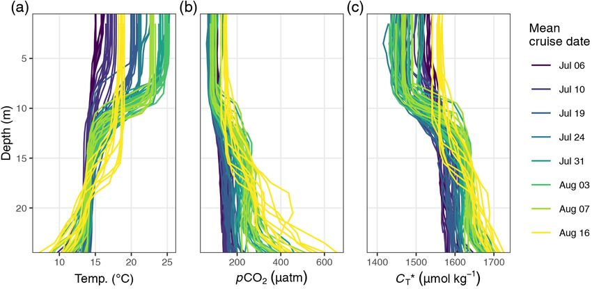
J. D. Müller et al.: Cyanobacteria NCP in the Baltic Sea                                                                           4893

Figure 1. (a) Extent of the cyanobacteria bloom on 26 July, detectable as greenish patterns in a true-colour satellite image (MODIS Aqua–
Terra, NASA Worldview) showing the Central Baltic Sea around the island of Gotland. The box indicates the study area as shown in (b),
a bathymetric map with the cruise tracks of SV Tina V (BloomSail campaign) and SOOP Finnmaid. BloomSail stations and the SOOP
sub-transects used in this study are highlighted in red. The ICOS flux tower for atmospheric measurements is located on the island of
Östergarnsholm.

started after complete equilibration of the pCO2 sensor in             ratory within no more than 21 d after sampling. CT was de-
near-surface waters, the applied response time correction has          termined with an automated infrared inorganic carbon anal-
only a minor impact on the derived NCP estimate.                       yser (AIRICA, Marianda, Kiel, Germany), and AT was anal-
                                                                       ysed by open cell titration (Dickson et al., 2007). CT and AT
2.2.3   Discrete CT , AT , and phytoplankton sampling                  measurements were referenced to certified reference mate-
                                                                       rials from batch 173 (Dickson et al., 2003). The mean ob-
Discrete water samples were collected with a manually re-              served AT was used for the calculation of CT∗ from pCO2
leased Niskin bottle. The sampling was restricted to stations          (see Sect. 2.5.2), while measured CT was only used for com-
07 and 10 (Fig. 1b) due to logistic constraints. The sam-              parison to calculated values and not directly included in the
pling depth was estimated based on the length of the released          NCP calculation. Phytoplankton samples were fixed with Lu-
line. CT and AT samples were filled into 250 mL SCHOTT-                gol solution, and cyanobacteria community composition and
DURAN bottles and poisoned with 200 µL saturated HgCl2                 biomass were determined by microscopic counts of the gen-
solution within 24 h after sampling. Samples were stored               era Aphanizomenon, Dolichospermum, and Nodularia ac-
dark and cool, transported to IOW, and analysed in the labo-

https://doi.org/10.5194/bg-18-4889-2021                                                        Biogeosciences, 18, 4889–4917, 2021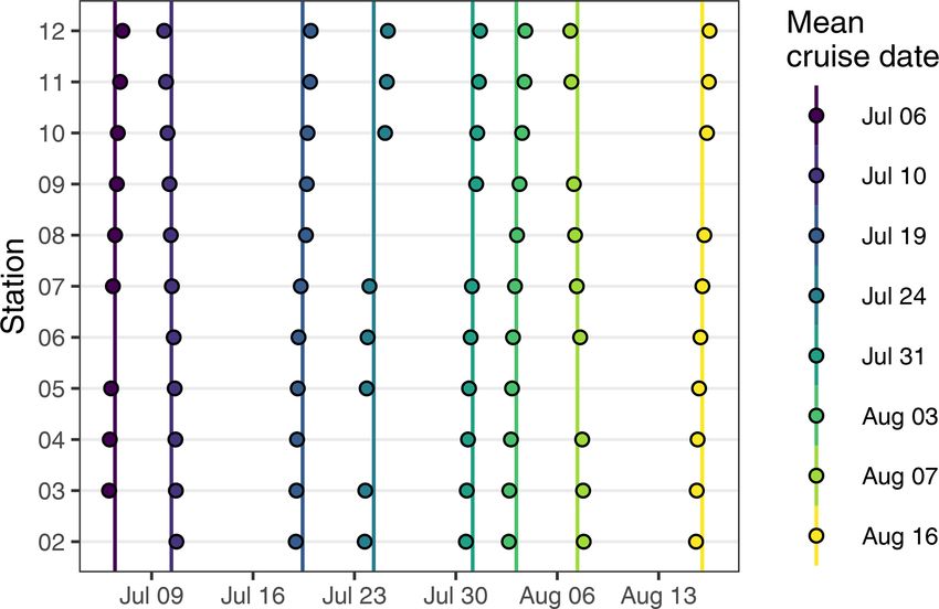
4894                                                                    J. D. Müller et al.: Cyanobacteria NCP in the Baltic Sea

                                                                       CT∗ is below 2 µmol kg−1 when the mean AT is constrained
                                                                       within the observed standard deviation of ±27 µmol kg−1
                                                                       (see Appendix C1 for a detailed assessment).

                                                                       2.5     NCP best guess

                                                                       The determination of our NCP best guess relies on the inter-
                                                                       pretation of observed temporal changes in CT∗ (1CT∗ ) across
                                                                       the water column. Conceptually, our calculations follow the
                                                                       idea of a one-dimensional box model approach, which does
                                                                       not resolve regional variability within the research area; i.e.
                                                                       it neglects lateral water mass transport. The calculation of
                                                                       the underlying 1CT∗ profiles requires a vertical gridding
                                                                       of measured profiles into discrete depth intervals δz and
Figure 2. Overview on profiling sensor measurements performed at       their regional averaging across all stations (for details see
stations 02–12 (Fig. 1). Individual sampling events are displayed as   Sect. 2.5.1). According to Eq. (1), we derive the column in-
points, whereas vertical lines indicate the mean date of each cruise   ventory of incremental changes of 1CT∗ (i1CT∗ ) between two
event.                                                                 cruise events through vertical integration of 1CT∗ from the
                                                                       sea surface to the compensation depth (CD), i.e. the depth
                                                                       (z) at which no net drawdown of CO2 was observed:
cording to the Utermöhl method (HELCOM, 2017). For de-
                                                                                   CD
tails on the analysis of discrete samples, see Appendix B.             i1CT * =
                                                                                   X
                                                                                          1CT *(z)δz.                             (1)
                                                                                  z=0 m
2.3    Atmospheric measurements
                                                                          Correcting i1CT∗ for the cumulative CO2 fluxes between
Meteorological observations were provided by the ICOS                  two cruise events caused by air–sea gas exchange (Fair-sea ;
flux tower (Fig. 1b) located on the southernmost tip of the            see Sect. 2.5.2) and vertical mixing (Fmix , see Sect. 2.5.3)
Island of Östergarnsholm (57.43010◦ N, 18.98415◦ E; Rut-               leads to incremental NCP estimates according to
gersson et al., 2020). Atmospheric pCO2,atm was recorded               NCPbest guess = −i1CT * − Fair-sea − Fmix .                (2)
with an atmospheric profile system (AP200, Campbell Sci-
entific, Logan, USA) mounted with a CO2 –H2 O gas anal-                   Incremental NCP estimates between cruise events are fur-
yser (LI-840A, LI-COR Biosciences, Lincoln, USA). Wind                 ther added up to derive cumulative NCP over the study pe-
speed was measured with a wind monitor (Young, Michigan,               riod. We refer to the derived NCP estimate as our best guess,
USA) at 12 m above mean sea level. Wind speed and pCO2                 as it is well-constrained by high-quality measurements and
data were averaged over 30 min intervals for further analysis.         therefore as close to the truth as currently possible.
Measured wind speed was converted to U10 , the wind speed              2.5.1    Vertical gridding and regional averaging
at 10 m a.s.l. (Winslow et al., 2016), to be consistent with the
gas exchange parameterisation (see Sect. 2.5.2).                       The vertical gridding of individual profiles was achieved by
                                                                       calculating mean values within depth intervals (δz) of 1 m.
2.4    CT∗ calculation                                                 Downcast profiles with missing observations from two or
                                                                       more depth intervals caused by zeroing measurements of the
The dissolved inorganic carbon concentration (CT∗ ) was                pCO2 sensor were discarded, which affected 8 out of 86
calculated from the measured profiles of temperature and               recorded profiles. For each of eight cruise events (Fig. 2),
response-time-corrected pCO2 (Schneider et al., 2014), as              regionally averaged profiles were further calculated as mean
well as the mean AT (1720 µmol kg−1 ) and mean salinity                values within each depth interval across all stations. Based
(6.9) determined from discrete samples collected across the            on those mean, vertically gridded cruise profiles, incremental
upper 20 m of the water column and over the entire observa-            and cumulative changes over time were calculated for each
tion period (Fig. B1). Calculations were performed with the            depth interval. Throughout the paper, observations averaged
R package seacarb (Gattuso et al., 2020), using the CO2 dis-           across the upper 0–6 m of the water column are referred to as
sociation constants for estuarine waters from Millero (2010).          surface observations.
   The calculated CT∗ represents an alkalinity- and salinity-
normalised estimate of the dissolved inorganic carbon con-             2.5.2    Air–sea CO2 flux
centration. CT∗ is suitable to accurately determine changes
rather than absolute values of the dissolved inorganic carbon          The air–sea gas exchange of CO2 (Fair-sea ) was calculated
concentration and therefore the preferred variable to quan-            from sea surface pCO2 , salinity, and temperature, in com-
tify NCP. The uncertainty in the determination of changes of           bination with pCO2,atm and U10 according to Wanninkhof

Biogeosciences, 18, 4889–4917, 2021                                                         https://doi.org/10.5194/bg-18-4889-2021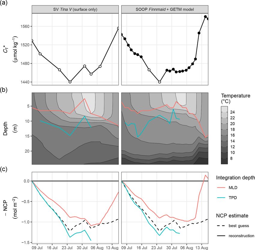
J. D. Müller et al.: Cyanobacteria NCP in the Baltic Sea                                                                  4895

(2014). For the calculation, sea surface observations were       Sect. 2.5.3). Based on all possible combinations of two CT∗
linearly interpolated to match the temporal resolution of at-    time series and two integration depth constraints, four recon-
mospheric measurements. A negative sign of Fair-sea indi-        structed NCP time series were derived and compared to the
cates uptake of CO2 from the atmosphere.                         best guess (i.e. the estimate based on the vertically resolved
                                                                 pCO2 observations from this study).
2.5.3    Vertical entrainment flux of CO2 through mixing
                                                                 2.6.1   SOOP Finnmaid surface pCO2
Between 6 June and 7 August, vertical mixing of CT∗ into the
surface layer (Fmix ) was neglected, because a stable thermo-    SOOP Finnmaid regularly commutes between Helsinki in
cline coincided with the integration depth for the NCP calcu-    Finland and Travemünde in Germany, thereby crossing the
lation (i.e. the compensation depth). However, clear signals     entire Central Baltic Sea and our study area on the east coast
for significant vertical entrainment of CT∗ across this layer    of Gotland every 1–2 d. On board SOOP Finnmaid, pCO2
were observed between 7 and 16 August (Fig. 3). This en-         is measured with a bubble-type equilibrator system supplied
trainment was quantified assuming an instantaneous com-          with water from an inlet at around 3 m water depth. De-
plete vertical mixing to 17 m water depth after 7 August. For    tails of the measurement set-up are described in Schneider
this simplified scenario, Fmix was estimated based on a mass     et al. (2014), and data are submitted on a regular basis to the
balance of CT∗ , which behaves conservatively with respect       Surface Ocean CO2 Atlas SOCAT (Bakker et al., 2016). The
to mixing (see Appendix C2 for details). A negative sign of      primary measurement system used to determine pCO2 in this
Fmix indicates entrainment of CO2 into the surface layer.        study is a NDIR sensor (LI-6262, LI-COR Biosciences, Lin-
                                                                 coln, USA). The ferrybox unit is also equipped with an ad-
2.6     NCP reconstruction from surface pCO2
                                                                 ditional methane–carbon dioxide analyser (greenhouse gas
        observations and hydrographical profiles
                                                                 analyser DLT 100, type 908-0011, Los Gatos Research, San
Our calculation of depth-integrated NCP from a time series       Jose, USA), providing independent pCO2 observations (Gül-
of surface pCO2 observations, such as provided by SOOP,          zow et al., 2011). Intercomparison of both systems is rou-
also relies on the conversion of pCO2 to CT∗ . Incremental       tinely used to ensure the correct functioning of the instru-
changes of CT∗ in the surface water further need to be multi-    mentation. In this study, a data gap caused by malfunction-
plied with an estimate of the integration depth (ID) to de-      ing of the primary LI-COR system was filled by including
rive an inventory change. Taking the air–sea flux of CO2         data recorded with the Los Gatos system on six cruises be-
(Sect. 2.5.2) into account, the NCP reconstruction can be de-    tween 8 and 16 July (see Appendix D for details). The mean
termined as                                                      regional pCO2 , sea surface temperature (SST), and salinity
                                                                 (SSS) were calculated for each crossing of the study area
NCPreconstruction = −1CT *surface · ID − Fair-sea .        (3)   (Fig. 1b). Based on the mean pCO2 and SST values, CT∗ was
                                                                 calculated following the procedure outlined in Sect. 2.4. A
   In the lack of vertical CT∗ observations, we tested two al-   remaining gap in the SOOP time series was filled with two in
ternative approximations of ID, which are                        situ CT∗ observations from the BloomSail campaign (19 and
                                                                 24 July).
• mixed-layer depth (MLD) and
• temperature penetration depth (TPD).                           2.6.2   GETM model temperature and salinity

  MLD and TPD are described in detail in Sect. 2.6.3. The        Surface SOOP measurements were complemented with ver-
two parameterisations were further applied to the following      tically resolved salinity and temperature data from the out-
two test data sets, both of which contain the required surface   put of a numerical ocean model of the Baltic Sea. The de-
pCO2 and vertically resolved temperature and salinity data:      ployed General Estuarine Turbulence Model (GETM) has
                                                                 a horizontal resolution of 1 nautical mile and 50 vertical
• in situ data from the BloomSail campaign without pCO2          terrain-following levels. The uppermost level has a thick-
     data at depth (SV Tina V (surface only))                    ness of maximum 50 cm to properly represent SST and
• combined SOOP surface pCO2 observations and mod-               ocean–atmosphere fluxes. The computation of the atmo-
    elled salinity and temperature profiles (SOOP Finn-          spheric fluxes is based on the parameterisation of Kara et al.
    maid + GETM model).                                          (2005). The model covers the entire Baltic Sea and the period
                                                                 1961–2019. A detailed analysis of the model performance is
   For both data sets, CT∗ time series were calculated based     given in Placke et al. (2018) and Gräwe et al. (2019). For the
on the same observed mean AT as used to derive the NCP           present study, we used a model run restarted in 2003 with
best guess (Sect. 2.4). Please note that neither the MLD nor     the atmospheric forcing from the operational reanalysis data
the TPD approach allows us to resolve vertical entrainment       set of the German weather service (Zängl et al., 2015). Addi-
fluxes, because profiles of CT∗ are not reconstructed (compare   tionally, we implemented the Langmuir-circulation parame-

https://doi.org/10.5194/bg-18-4889-2021                                                 Biogeosciences, 18, 4889–4917, 2021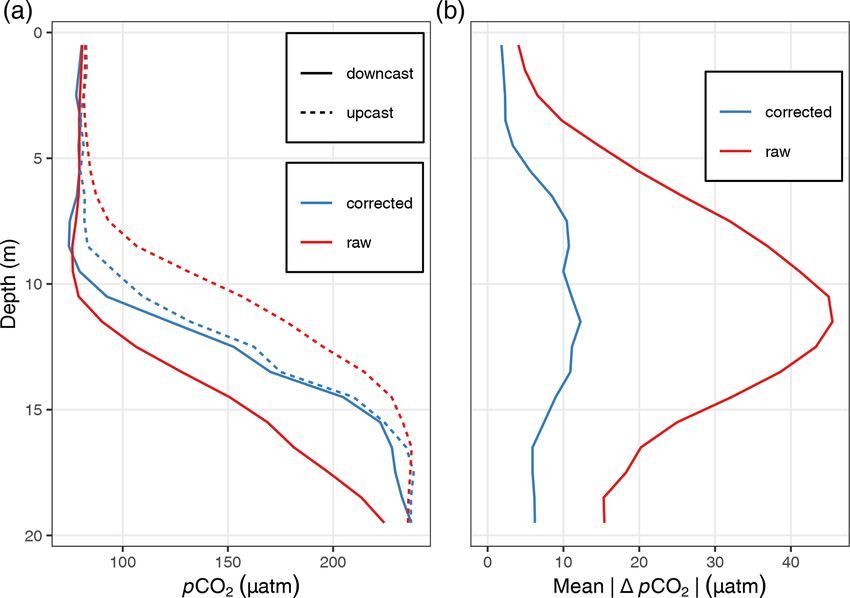
4896 J. D. Müller et al.: Cyanobacteria NCP in the Baltic Sea
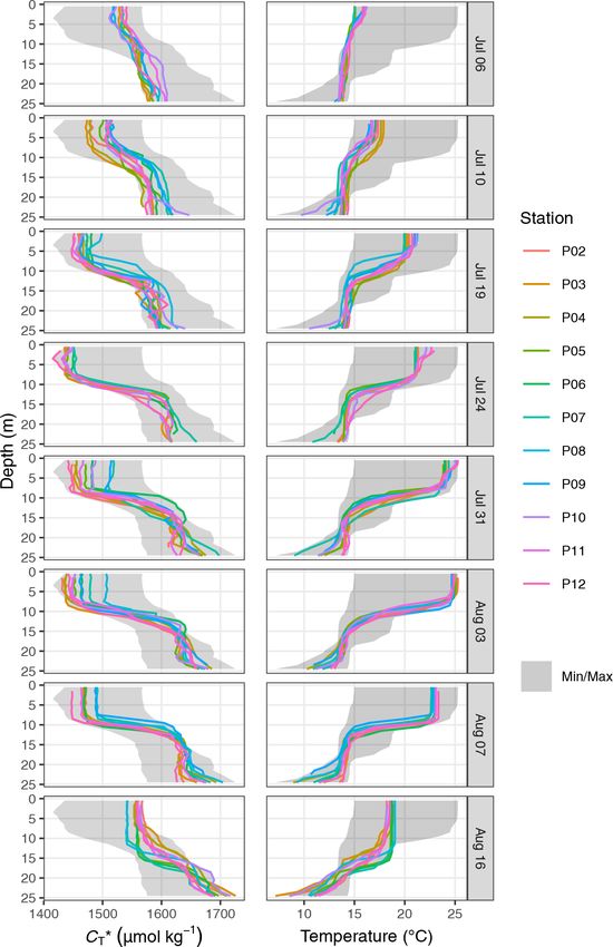
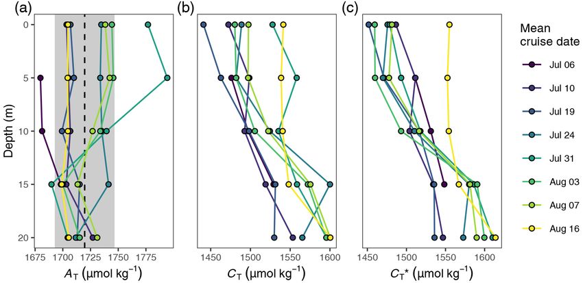
Figure 3. Overview of (a) temperature, (b) pCO2 , and (c) CT∗ profiles recorded throughout the BloomSail field sampling campaign on board
SV Tina V.
terisation of Axell (2002), to account for wind-wave-induced that ceases abruptly at 10 m water depth would result in the
variation in the mixed-layer depth. Model results were aver- same TPD as a warming signal that decreases linearly from
aged over 24 h and interpolated to a standardised section with the surface to 20 m water depth (TPD is 10 m in both cases).
2 km horizontal and 1 m vertical resolution, which follows The TPD approach is motivated by the assumption that pri-
the mean Finnmaid cruise track. Based on this standard sec- mary production and temperature increase are both primar-
tion, daily mean profiles within the study area (characterised ily controlled by the light dose that a water parcel received
by little regional variability) were computed and linearly in- (Schneider et al., 2014) and therefore show similar vertical
terpolated to match the exact times of Finnmaid crossings. patterns.
In analogy to TPD, the penetration depth of CT∗ drawdown
2.6.3 Parameterisation of the integration depth (ID) (CPD) was defined as the integrated loss of CT∗ across the
water column divided by the decrease in CT∗ at the surface
In this study, two parameters were used to integrate surface (Fig. C4b).
observations across depth, namely the classical mixed-layer
depth (MLD) and the newly introduced temperature penetra- 3 Results
tion depth (TPD).
MLD was defined as the shallowest depth at which seawa- 3.1 Dynamics of temperature, pCO2 , CT∗ , and
ter density exceeds the density at the surface by more than phytoplankton biomass
0.1 kg m−3 (Roquet et al., 2015). According to this defini-
tion, MLD characterises the thermohaline structure of the Between 6 July and 16 August, a total number of 78
water column and often (but not necessarily) approximates complete vertical CTD and pCO2 downcast profiles were
the depth to which surface water masses are actively mixed. recorded (Figs. 2 and 3). CT∗ was calculated and profiles
The definition through a fixed density threshold further im- were regionally averaged for each of the eight cruise events
plies that gradual changes of temperature with depth are not (Fig. 4). Since the first cruise of the BloomSail expedition
reflected by this parameter. on 6 July, sea surface temperature (SST) increased steadily
TPD characterises the mean penetration depth of surface from ∼ 15 ◦ C to peak values of ∼ 25 ◦ C (Figs. 4 and 5) ob-
warming that occurred between two sampling events. TPD served on 3 August. Sea surface pCO2 was already as low as
was defined as the integrated warming signal across the wa- ∼ 100 µatm at the beginning of July (Fig. 5a) and decreased
ter column, i.e. the sum of all positive temperature changes further to the lowest values of ∼ 70 µatm on 24 July. The drop
within 1 m depth intervals, divided by the SST increase (for in pCO2 and the simultaneous increase in SST correspond to
a graphical illustration see Fig. C4a). According to this defi- a decrease in CT∗ of almost 90 µmol kg−1 (Fig. 4). During this
nition and in contrast to MLD, TPD takes gradual changes of period of intense primary production, the regional variability
temperature across depth into account and does not require of SST, pCO2 , and CT∗ across stations was low compared to
a fixed threshold value. TPD is only applicable when SST their temporal change (Figs. 5a and b; and C3). The regional
increases and has units of metres. To illustrate the TPD con- variability is slightly higher when including the coastal sta-
cept, it should be noted that a homogeneous warming signal tions 01, 13, and 14 (results not shown) but is generally lower
Biogeosciences, 18, 4889–4917, 2021 https://doi.org/10.5194/bg-18-4889-2021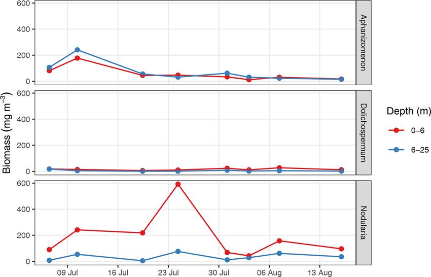
J. D. Müller et al.: Cyanobacteria NCP in the Baltic Sea                                                                     4897

than one could expect from the bloom patchiness typically         3.2   NCP best guess based on profiling measurements
observed through remote sensing (Fig. 1a). With respect to
pCO2 dynamics, it should be noted that (i) the observed tem-      Net community production (NCP) was determined through
perature increase and CT∗ drawdown have opposing effects on       vertical integration of the observed drawdown of CT∗ from
pCO2 , and (ii) the change of pCO2 per change in CT∗ is gen-      the surface to the compensation depth located at 12 m. The
erally low at low absolute pCO2 . The observed CT∗ dynam-         determined compensation depth reflects the maximum pen-
ics in surface waters are clearly attributable to the primary     etration depth of the incremental (i.e. between cruise days),
production activity of phytoplankton and go along with an         as well as the cumulative (i.e. from 6–24 July), CT∗ draw-
observed increase in the biomass of Nodularia sp. (Fig. B2),      down (Fig. 4). Likewise, about 95 % of the cumulative warm-
which also peaked on 24 July. Furthermore, we found that CT∗      ing signal, which refers to positive temperature changes inte-
calculated from pCO2 agreed with CT∗ derived from discrete        grated over depth, occurred above 12 m.
samples within the uncertainty range attributed to regional          Until 24 July, the depth-integrated CT∗ drawdown
variability (Fig. 5c).                                            amounted to ∼ 0.9 mol m−2 (Fig. 5h). This observed CT∗
   Between the extremes of pCO2 and CT∗ (minimum on               drawdown was corrected for air–sea fluxes of CO2 . Between
24 July) and SST (maximum on 3 August), a noticeable in-          6 July and 7 August, the cumulative air–sea flux (Fair-sea, cum )
crease in surface CT∗ was observed on 31 July, which was          amounted to around −0.5 mol m−2 (Fig. 5g), with a negative
accompanied by a higher regional variability across the sta-      sign representing CO2 uptake from the atmosphere. In the
tion network (Fig. 5a and c). The temporary CT∗ increase was      absence of noticeable vertical mixing, this flux was entirely
limited to the north-eastern stations 07–10 (Fig. C3) and par-    added to the observed CT∗ drawdown. Only between 7 and
alleled by a drop in salinity and elevated AT at the same         16 August, when mixing to about 17 m water depth was ob-
stations (Fig. B1). It is therefore attributable to the lateral   served, was a significant fraction of the CO2 taken up from
exchange of water masses. All signals of this lateral intru-      the atmosphere transported below 12 m water depth. To ac-
sion vanished within a week. At the other stations (02–06         count for the partial loss of airborne CO2 to deeper waters
and 11–12), no noticeable signs of water mass exchange or         during this 9 d period, only 12/17 of Fair-sea, cum during this
CT∗ changes were observed between 24 July and 3 August, in-       time (−0.2 mol m−2 ), which is the fraction that would remain
dicating that the production and respiration of organic matter    in the upper water column, was added to the observed CT∗
were balanced during this period. During the first 2 weeks of     drawdown. In addition, a significant amount of CT∗ entrain-
August the study area was affected by increased wind speeds,      ment (−0.5 mol m−2 ) into the surface layer was caused by
causing a decrease in SST back to ∼ 18 ◦ C. The simultane-        the vertical mixing between 7 and 16 August (Figs. 5h and
ous return of surface pCO2 to ∼ 150 µatm corresponded to a        C2).
CT∗ increase of ∼ 100 µmol kg−1 .                                    After correction for air–sea fluxes and vertical entrain-
   The observed surface warming and CT∗ drawdown ex-              ment of CO2 , the cumulative changes of depth-integrated
tended vertically to a water depth of ∼ 10 m (Fig. 4). On         CT∗ represent the NCP between the sea surface and the com-
the first cruise day (6 July), the vertical distribution of CT∗   pensation depth at 12 m (Fig. 5h). The peak NCP value of
and temperature was still relatively homogeneous. CT∗ at          ∼ 1.2 mol m−2 was observed on 24 July and is of primary in-
25 m water depth was ∼ 70 µmol kg−1 higher than at the sur-       terest because it reflects the amount of organic matter that
face. Likewise, the temperature gradient covered only ∼ 3 ◦ C     was produced and is potentially available to be either ex-
from 16 ◦ C at the very surface to 13 ◦ C at depth. The warm-     ported or remineralised. The temporary drop in the NCP
ing of surface waters caused an increasingly stable thermo-       best guess on 31 July is due to the lateral exchange of wa-
cline to be established at around 10 m water depth, which         ter masses as described in Sect. 3.1. Deriving the NCP time
reached a temperature gradient of ∼ 10 ◦ C across 5 m on          series without the stations affected by later exchange of wa-
3 August. Likewise, continuous and uniform drawdown of            ter masses (07–10) results in an almost identical NCP es-
CT∗ within the surface layer enhanced the vertical CT∗ gradi-     timate on 24 July but a reduced drop on 31 July (data not
ent to > 150 µmol kg−1 between the surface and 25 m water         shown). In both cases, no signs of continued NCP were ob-
depth. The CT∗ drawdown was observed to a maximum depth           served after 24 July. Accordingly, our interpretation of the
of 12 m.                                                          reconstructed NCP based on surface pCO2 observations will
   Between 7 and 16 August the SST drop of ∼ 6◦ C was ac-         focus on the comparison to the peak value of our NCP best
companied by a temperature increase in deeper water layers        guess on 24 July.
(11–17 m) of up to 5 ◦ C. This vertical redistribution of heat
indicates vertical mixing of water masses, which was also
reflected in a steep increase in CT∗ in the surface water and a
loss of CT∗ between 11–17 m (Figs. 3 and 4).

https://doi.org/10.5194/bg-18-4889-2021                                                  Biogeosciences, 18, 4889–4917, 2021
4898 J. D. Müller et al.: Cyanobacteria NCP in the Baltic Sea
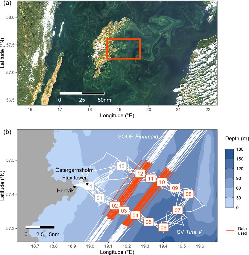
Figure 4. (a) Temperature and (b) CT∗ between 6 July and 16 August displayed as (1) Hovmöller plots and (2) profiles of cumulative
changes since the first cruise on 6 July. Mean cruise dates are indicated by the horizontal position of white symbols in (a1) and (b1), and the
compensation depth of 12 m is indicated as a red horizontal line in (a2) and (b2).
3.3 NCP reconstruction based on surface pCO2 and very similar increase in CT∗ between 6 and 15 August was
hydrographical profiles determined from both independent observational data sets.
The good agreement between the independent observations
The reconstruction of depth-integrated NCP was tested for justifies that a data gap due to failure of instrumentation on
two data sets containing the same type of information, the SOOP was filled with two observations from SV Tina V
namely the observed changes in surface pCO2 and vertical on 19 and 24 July (open circles in Fig. 6a).
profiles of seawater salinity and temperature. The first data Good agreement was also found for the spatio-temporal
set “SV Tina V (surface only)” contains the surface pCO2 dynamics of observed and modelled seawater temperature
data recorded during the BloomSail expedition, as well as the (Fig. 6b). Observed and modelled SST agreed within 1 ◦ C
complete CTD profiles. The second data set (“SOOP Finn- over the entire observation period, despite an absolute change
maid + GETM model”) combines surface pCO2 observa- spanning almost 10 ◦ C. Slightly higher deviations between
tions from SOOP Finnmaid with seawater salinity and tem- observed and modelled temperature were found around
perature as estimated with the GETM model. the thermocline, where the observational record revealed a
An almost identical decrease in surface CT∗ of ∼ stronger temperature gradient. This difference is likely due
50 µmol kg−1 was determined between 6 and 16 July to an imperfect representation of Langmuir circulation in
(Fig. 6a), based on the completely independent pCO2 data the model (Axell, 2002), whereas the absence of increased
recorded on SOOP Finnmaid and SV Tina V. Likewise, a light attenuation caused by phytoplankton particles was pre-
Biogeosciences, 18, 4889–4917, 2021 https://doi.org/10.5194/bg-18-4889-2021J. D. Müller et al.: Cyanobacteria NCP in the Baltic Sea 4899 Figure 5. Time series displaying from top to bottom sea surface observation of (a) pCO2 , (b) temperature, and (c) CT∗ with grey ribbons in- dicating the standard deviation across stations and red symbols representing discrete sample data; atmospheric observations of (d) pCO2,atm , (e) wind speed at 10 m, (f) daily and (g) cumulative air–sea fluxes of CO2 ; and (h) the derived water column inventory changes of CT∗ . In (h), bars represent incremental changes between cruise events (vertical grid lines), whereas lines represent cumulative changes since the first cruise. Colours distinguish observed CT∗ changes from values referring to the applied air–sea CO2 flux and mixing correction. Net community production (NCP) is equal to the negative value of flux and mixing-corrected cumulative changes of CT∗ (purple line) and peaks on 24 July. https://doi.org/10.5194/bg-18-4889-2021 Biogeosciences, 18, 4889–4917, 2021
4900                                                                     J. D. Müller et al.: Cyanobacteria NCP in the Baltic Sea

Figure 6. Time series illustrating the reconstruction of depth-integrated NCP from surface CT∗ and vertically resolved hydrographical pa-
rameters. Displayed are results based on two test data sets, namely observations from SV Tina V without CT∗ data at depth (left panels) and
a combination of SOOP CT∗ and modelled hydrographical data (right panels). From top to bottom, panels represent (a) surface CT∗ , (b) the
vertical distribution of temperature together with the mixed-layer depth (MLD) and temperature penetration depth (TPD) for each cruise day,
and (c) depth-integrated NCP comparing the reconstructions (solid lines) with the best guess (dashed black line) according to Fig. 5. Please
note that a data gap in the SOOP record was filled with two observations from SV Tina V (open circles in a).

viously found to have only minor impacts on modelled SST                   Based on SOOP observations before 6 July, first signs of
dynamics (Löptien and Meier, 2011). Most importantly, the               the onset of the investigated bloom event were detected al-
mean temperature penetration depths (TPDs) derived from                 ready on 3 July. Between 3 and 6 July, an SST increase of ∼
the observational and model data differ by less than 1 m,               1 ◦ C was accompanied by a CT∗ drawdown of ∼ 10 µmol kg−1
indicating that surface warming and the integrated heat up-             (data not shown). Still, in the absence of any vertically re-
take are accurately represented by the model. The TPD                   solved observation for this time period, the following com-
(mean ± SD) over the observed productive period between                 parison of the reconstructions to the best guess needs to be
6 and 24 July was determined as 12.3 ± 2.5 and 11.4 ± 2.3 m             restricted to the period 6–24 July, during which the bulk of
for the observational and model data, respectively (Fig. 6b).           NCP occurred.
The TPD estimates are considerably higher than the re-                     The NCP reconstruction based on TPD is generally higher
spective mixed-layer depth (MLD) estimates (6.0 ± 1.9 and               than the MLD-based estimate (Fig. 6c). Comparing peak cu-
5.5 ± 1.2 m) and agree better with the observed penetration             mulative NCP estimates for 24 July, the TPD approach re-
depth of CT∗ drawdown, indicating that TPD is the favourable            sults in a ∼ 10 % overestimation compared to the best guess,
parameterisation of the integration depth.                              i.e. the value derived from vertically resolved measurements.

Biogeosciences, 18, 4889–4917, 2021                                                         https://doi.org/10.5194/bg-18-4889-2021
J. D. Müller et al.: Cyanobacteria NCP in the Baltic Sea                                                                         4901

In contrast, the MLD-based NCP estimate is ∼ 30 % lower              pulses observed in the years 2005, 2008, 2009, and 2011, the
than the best guess. The reconstructed NCP estimates are             authors found average daily rates of CT∗ drawdown ranging
very similar for both test data sets, as the good agreement          from 3 to 8 µmol kg−1 d−1 , which comprises the mean rate
between the underlying CT∗ , MLD, and TPD time series sug-           of 5 µmol kg−1 d−1 determined in this study (i.e. the average
gests.                                                               CT∗ drawdown of ∼ 90 µmol kg−1 over 18 d, Fig. 4). The indi-
   Comparing the deviation between the best guess and re-            vidual production events identified by Schneider et al. (2014)
constructed NCP estimates in light of the lateral variabil-          lasted 1 to 5 weeks, similar to the bloom duration described
ity observed within the study area, it must be emphasised            in this study. Finally, Schneider et al. (2014) also provided
that between 6 and 24 July, the mean standard deviation              a depth-integrated NCP estimate based on daily modelled
of pCO2 and CT∗ across stations amounted to ±6 µatm                  mixing depths, which ranged from 3–20 m and were derived
and ±11 µmol kg−1 , respectively. This is higher than the            from the vertical distribution of a tracer 1 d after its injection
likely uncertainty associated with the pCO2 measurements             into the surface. Although this approach is primarily useful
(see Methods), as well as its response time correction (see          to estimate the vertical distribution of air–sea CO2 fluxes and
Methods and Appendix A4) or conversion to CT∗ (see Ap-               does not necessarily reflect the vertical extent of organic mat-
pendix C1). Therefore, the lateral variability of seawater           ter production, their determined midsummer NCP estimates
chemistry and the production signal are generally considered         (1–2.1 mol m−2 ) are on the same order of magnitude as the
the highest source of uncertainty to our NCP estimates. Still,       best guess derived in this study. It should be noted that the
this lateral variability is small compared to the signal to be re-   NCP estimates by Schneider et al. (2014) refer to the cumula-
solved (i.e. the CT∗ drawdown of ∼ 90 µmol kg−1 ). However,          tive NCP of one to three production pulses per year, whereas
on a relative scale the lateral CT∗ variability is about as large    our estimate of ∼ 1.2 mol m−2 refers to a single bloom event.
as the difference between the best guess and the TPD-based              Wasmund et al. (2001) conducted 14 C incubation exper-
NCP reconstruction (∼ 10 %), suggesting that the bias of the         iments at different water depths to determine instantaneous
reconstruction falls within the uncertainty range of the best        rates of daytime primary production during a cyanobacteria
guess. In contrast, the lateral variability is smaller than the      bloom. Their reported carbon fixation rates in surface wa-
deviation between the best guess and the MLD-based NCP               ters (0.4–0.8 mmol m−3 h−1 ) are on the same order of mag-
reconstruction.                                                      nitude as the mean rate found in this study (5 µmol kg−1 d−1 ,
   All reconstructed NCP estimates include the correction of         equivalent to 0.2 mmol m−3 h−1 ), despite representing day-
air–sea fluxes of CO2 , but it is impossible to quantify and         time production rates and diurnal averages. More important
correct vertical entrainment fluxes due to mixing, because           than the agreement between the fixation rates at the sea sur-
the vertical distribution of CT∗ across the water column can         face, is the fact that Wasmund et al. (2001) also found signif-
not be resolved. The strong deviation between the best guess         icantly lower carbon fixation rates below 10 m water depth
NCP and the MLD-based reconstruction on 16 August is due             (< 0.2 mmol m−3 h−1 ), which agrees well with the depth dis-
to this missing correction of vertical mixing. This deviation        tribution of NCP observed in this study.
highlights that the reconstruction approach is only applica-            Furthermore, the succession of different cyanobacteria
ble to production periods with a stable or shoaling thermo-          genera observed in 2018, with the Nodularia-dominated
cline. The TPD-based approach does not allow for any esti-           bloom following an earlier presence of Aphanizomenon
mate during the last 2 weeks of the observation period, as the       (Fig. B2), was previously described as a typical pattern (Was-
TPD is per definition only applicable to periods of warming          mund, 2017), as well as the fact that increased wind speed
surface waters.                                                      and turbulence can inhibit N fixation of cyanobacteria and
                                                                     cause the termination of the bloom (Wasmund, 1997).
                                                                        In conclusion, the bloom event duration, CT∗ drawdown,
4     Discussion                                                     and NCP, as well as the vertical extent of carbon fixation
                                                                     and the succession of the bloom observed in this study, agree
4.1    Comparison to previous studies                                well with observations in previous years, and distinct differ-
                                                                     ences cannot be found. We therefore conclude that the find-
Having in mind the application of our NCP reconstruction             ings of this study are representative for Baltic Sea cyanobac-
approach to surface pCO2 observation collected since 2003,           teria blooms in general, although the SST and pCO2 levels
it is important to examine whether the biogeochemical dy-            in 2018 were at the upper and lower ends, respectively, of the
namics of the examined cyanobacteria bloom in 2018 is rep-           conditions observed in previous years (Schneider and Müller,
resentative for those in other years. Unfortunately, only a few      2018).
previous studies aimed at the quantification of cyanobacteria
growth as a component of the Baltic Sea carbon budget. One           4.2   Biogeochemical relevance and interpretation
exception is the interpretation of SOOP Finnmaid data by
Schneider et al. (2014). Focusing on the period from June to         Our best guess of cumulative NCP on 24 July
August and taking into consideration individual production           (∼ 1.2 mol m−2 ) represents the net amount of organic

https://doi.org/10.5194/bg-18-4889-2021                                                      Biogeosciences, 18, 4889–4917, 2021
4902 J. D. Müller et al.: Cyanobacteria NCP in the Baltic Sea
matter that was produced throughout the bloom event in SOOP infrastructure and help to provide the required obser-
the surface waters above the compensation depth at 12 m. vational constraints throughout the water column.
After subtracting ∼ 20 % dissolved organic carbon (DOC)
production (Hansell and Carlson, 1998; Schneider and Kuss, 4.3 Recommendations and caveats for NCP
2004), our NCP estimate equals the produced particulate reconstruction from SOOP and model data
organic carbon (POC) that is potentially available for export.
In contrast, NCP estimates derived from other traditional The good agreement between our best guess and the TPD-
methods for the integration across depth (such as the lower based NCP reconstruction on 24 July (Fig. 6c) indicates that
bound of the euphotic zone or the mixed-layer depth) would it is possible to determine NCP from surface pCO2 observa-
not directly relate to the POC export potential. tions and vertically resolved seawater temperature with little
However, the potential POC export constraint by our NCP uncertainty. For the NCP calculation based on surface pCO2
estimate is not equivalent to the supply of organic matter to observations from SOOP and modelled temperature profiles,
the deep waters of the Gotland Basin, because POC might we recommend
be (partly) remineralised before sinking beneath the perma- 1. converting surface pCO2 to CT∗ based on a mean AT
nent halocline. Remineralisation of POC that occurs during estimate for the region under consideration,
the bloom event above the compensation depth is – according
to our definition of NCP – already included in our estimate. 2. identifying production pulses dominated by cyanobac-
In contrast, any additional remineralisation of POC that oc- teria as periods characterised by a decrease in CT∗ that
curs between the compensation depth and the halocline, or occur between June and August,
above the compensation depth after the end of the bloom
event, reduces the organic matter supply to the deep waters 3. integrating observed surface CT∗ changes to the temper-
and thereby mitigates deoxygenation. Indeed, our profiling ature penetration depth (TPD) estimated from modelled
measurements indicate a steady accumulation of CT∗ beneath temperature profiles, rather than using a mixed-layer
the compensation depth (Fig. 4), likely fuelled by the rem- depth (MLD) estimate, and
ineralisation of organic matter. However, our measurements 4. performing the integration individually for each produc-
do not allow the constraint of the budget of this CT∗ accu- tion pulse and limiting NCP reconstruction to periods
mulation, and we could not attribute the source of organic characterised by a stable or shoaling thermocline.
matter.
In contrast to shallow remineralisation processes, the It should be emphasised that lateral variability and water
deepening of the mixed layer that marked the end of the mass transport are critical for observation-based NCP es-
studied bloom event may facilitate the efficient transport of timates and constitute the largest source of uncertainty in
POC from the surface layer to depth. Focusing on the ac- our estimates. However, SOOP observations allow averaging
cumulation of remineralisation products beneath 150 m in of observations across large regions, which reduces the im-
the Gotland Basin, a previous study revealed that – in ac- pact of lateral water mass transport (Schneider and Müller,
cordance with the main input of POC during the productive 2018). The region for spatial averaging should be chosen
period – remineralisation rates exhibit a pronounced season- large enough to avoid as much as possible the influence of
ality (Schneider et al., 2010). This seasonality was found to lateral perturbations which depend on the surface dynamics
be most pronounced in the water layers closest to the sedi- and the biogeochemical gradients in the surrounding area.
ment surface, suggesting that beneath 150 m the remineral- Yet, the region for spatial averaging should be chosen small
isation takes place mainly at the sediment surface and is of enough to ensure that variations in pCO2 within the region
minor importance during particle sinking through the deep are small compared to the temporal changes of interest. An-
water column. The pronounced seasonality further confirms other critical aspect of the recommended NCP reconstruction
that surface organic matter production and deep water oxy- approach is the restriction to periods of a stable or shoaling
gen consumption are indeed tightly coupled, despite a poten- thermocline. While in principle it is possible that net organic
tial degradation of POC before export across the permanent matter production could also occur during periods of a deep-
halocline. ening thermocline, this process was neither observed in this
We conclude that NCP estimates determined with the study nor in previous years (Schneider and Müller, 2018)
methods developed in this study are of direct relevance to and is in line with findings from the long-term cyanobac-
quantify the drivers for deep water deoxygenation. How- teria monitoring programme unravelling that increased wind
ever, a better understanding of the organic matter reminer- speed causes the termination of the bloom (Wasmund, 1997).
alisation processes would be required to close the budget We thus conclude that reconstructed NCP estimates are not
of biogeochemical transformations. New observational plat- affected by a systematic underestimation due to this temporal
forms, such as recently deployed biogeochemical ARGO restriction. Likewise, the required mean AT estimate should
floats (Haavisto et al., 2018), will complement the existing not restrict the applicability of our approach even if AT is not
directly measured. For the Baltic Sea, it was demonstrated
Biogeosciences, 18, 4889–4917, 2021 https://doi.org/10.5194/bg-18-4889-2021You can also read