Data-Efficient Behavior Prediction for Safe Human-Robot Collaboration
←
→
Page content transcription
If your browser does not render page correctly, please read the page content below
Data-Efficient Behavior Prediction
for Safe Human-Robot Collaboration
                    Ruixuan Liu
              CMU-RI-TR-21-30
                   July 28, 2021

                The Robotics Institute
             School of Computer Science
             Carnegie Mellon University
                   Pittsburgh, PA
                 Thesis Committee:
                   Changliu Liu
                  Oliver Kroemer
                    Katia Sycara
                  Jaskaran Grover

  Submitted in partial fulfillment of the requirements
   for the degree of Master of Science in Robotics.
   Copyright © 2021 Ruixuan Liu. All rights reserved.
Abstract

Predicting human behavior is critical to facilitate safe and efficient human-
robot collaboration (HRC) due to frequent close interactions between humans
and robots. However, human behavior is difficult to predict since it is diverse
and time-variant in nature. In addition, human motion data is potentially
noisy due to the inevitable sensor noise. Therefore, it is expensive to collect a
motion dataset that comprehensively covers all possible scenarios. The high
cost of data collection leads to the scarcity of human motion data in certain
scenarios, and therefore, causes difficulties in constructing robust and reliable
behavior predictors. This thesis uses online adaptation (an online approach)
and data augmentation (an offline approach) to deal with the data scarcity
challenge in human motion prediction and intention prediction respectively.
This thesis proposes a novel adaptable human motion prediction framework,
RNNIK-MKF, which combines a recurrent neural network (RNN) and inverse
kinematics (IK) to predict human upper limb motion. A modified Kalman filter
(MKF) is applied to robustly adapt the model online to improve the prediction
accuracy, where the model is learned from scarce training data. In addition,
a novel training framework, iterative adversarial data augmentation (IADA),
is proposed to learn safe neural network classifiers for intention prediction.
The IADA uses data augmentation and expert guidance offline to augment
the scarce data during the training phase and learn robust neural network
models from the augmented data. The proposed RNNIK-MKF and IADA are
tested on a collected human motion dataset. The experiments demonstrate that
our methods can achieve more robust and accurate prediction performance
comparing to existing methods.

                                                                                    iii
iv
Acknowledgments

I would like to thank my advisor Professor Changliu Liu for her advice on my
work and continuous support of my Master’s study. She has been extremely
helpful, supportive, and patient throughout my study and I have learned a lot
from her insights in the research field.

I would also like to thank Professor Oliver Kroemer, Professor Katia Sycara,
and Jaskaran Grover for being my committee members. They provide a lot
of insightful comments on my work, which are really helpful for my future
research.

I want to also express my appreciation to my colleagues in the Intelligent
Control Lab and all the amazing people I met at the Robotics Institute.

Last but definitely not least, great thanks to my family and friends. I could never
achieve this without their unconditional support and understanding throughout
the journey.

                                                                                      v
vi
Funding

This work is in part supported by Ford Motor Company.

                                                        vii
viii
Contents

1   Introduction                                                                                                                         1
    1.1 Challenges . . . . . . . . . . . . . . . . . . . . . . . . . . . . . . . . . .                                                   2
    1.2 Motion Prediction . . . . . . . . . . . . . . . . . . . . . . . . . . . . . .                                                    3
    1.3 Intention Prediction . . . . . . . . . . . . . . . . . . . . . . . . . . . . .                                                   4

2   Related Work                                                                                                                         7
    2.1 Human Motion Prediction .        .   .   .   .   .   .   .   .   .   .   .   .   .   .   .   .   .   .   .   .   .   .   .   .   7
    2.2 Human Intention Prediction .     .   .   .   .   .   .   .   .   .   .   .   .   .   .   .   .   .   .   .   .   .   .   .   .   8
         2.2.1 Data Augmentation .       .   .   .   .   .   .   .   .   .   .   .   .   .   .   .   .   .   .   .   .   .   .   .   .   8
         2.2.2 Adversarial Training      .   .   .   .   .   .   .   .   .   .   .   .   .   .   .   .   .   .   .   .   .   .   .   .   8

3   Problem Formulation                                                                                                                  11
    3.1 Motion Prediction Formulation . . . . . . . . . . . . . . . . . . . . . . .                                                      11
    3.2 Intention Prediction Formulation . . . . . . . . . . . . . . . . . . . . . .                                                     13

4   Approach                                                                                                                             15
    4.1 RNNIK-MKF Motion Prediction . . . . . . . . . . . . .                                        .   .   .   .   .   .   .   .   .   15
        4.1.1 RNN for Wrist Motion Prediction . . . . . . . .                                        .   .   .   .   .   .   .   .   .   15
        4.1.2 IK for Arm Motion Prediction . . . . . . . . . .                                       .   .   .   .   .   .   .   .   .   17
        4.1.3 Online Adaptation with MKF . . . . . . . . . .                                         .   .   .   .   .   .   .   .   .   18
        4.1.4 Online Adaptation Estimation Error Propagation                                         .   .   .   .   .   .   .   .   .   19
    4.2 IADA Intention Prediction . . . . . . . . . . . . . . . .                                    .   .   .   .   .   .   .   .   .   22
        4.2.1 Formal Verification to Find Adversaries . . . . .                                      .   .   .   .   .   .   .   .   .   23
        4.2.2 Expert Guidance for Labeling . . . . . . . . . .                                       .   .   .   .   .   .   .   .   .   24
        4.2.3 Iterative Adversarial Data Augmentation . . . .                                        .   .   .   .   .   .   .   .   .   25
        4.2.4 Prediction Confidence Estimation . . . . . . . .                                       .   .   .   .   .   .   .   .   .   26
        4.2.5 IADA Analysis . . . . . . . . . . . . . . . . . .                                      .   .   .   .   .   .   .   .   .   27

5   Experiments                                                                                                                          29
    5.1 Data Collection . . . . . . . . . . . . . . . . . . . . . . . . . . . . . . .                                                    29
    5.2 RNNIK-MKF Motion Prediction . . . . . . . . . . . . . . . . . . . . . .                                                          30

                                                                                                                                         ix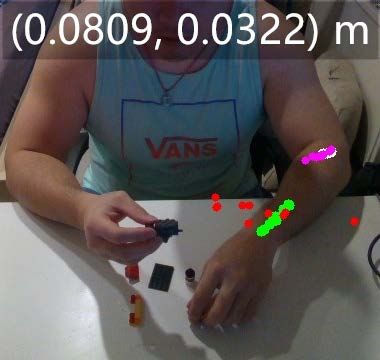
5.2.1 Prediction Experiments . . . . . . . . . . . . .     .   .   .   .   .   .   .   .   .   .   31
          5.2.2 Unseen Humans Experiments . . . . . . . . .          .   .   .   .   .   .   .   .   .   .   33
          5.2.3 Unseen Tasks Experiments . . . . . . . . . . .       .   .   .   .   .   .   .   .   .   .   35
          5.2.4 Motion Occlusion Experiments . . . . . . . .         .   .   .   .   .   .   .   .   .   .   36
          5.2.5 Online Adaptation Uncertainty . . . . . . . . .      .   .   .   .   .   .   .   .   .   .   37
    5.3   Intention Prediction with IADA . . . . . . . . . . . .     .   .   .   .   .   .   .   .   .   .   38
          5.3.1 2D Binary Classification . . . . . . . . . . . .     .   .   .   .   .   .   .   .   .   .   39
          5.3.2 2D Binary Classification with Biased Data . .        .   .   .   .   .   .   .   .   .   .   41
          5.3.3 MNIST . . . . . . . . . . . . . . . . . . . . .      .   .   .   .   .   .   .   .   .   .   43
          5.3.4 Intention Prediction . . . . . . . . . . . . . . .   .   .   .   .   .   .   .   .   .   .   44
          5.3.5 Intention Prediction Confidence . . . . . . . .      .   .   .   .   .   .   .   .   .   .   44
          5.3.6 Visualization of IADA for Intention Prediction       .   .   .   .   .   .   .   .   .   .   45
          5.3.7 Discussion . . . . . . . . . . . . . . . . . . .     .   .   .   .   .   .   .   .   .   .   48

6   Conclusion and Future Work                                                                               51

Bibliography                                                                                                 53

x
List of Figures
1.1 Visualizations of the human motion prediction using RNNIK-MKF. . . . 2
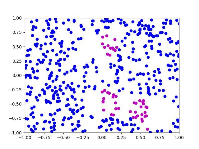
1.2 Visualizations of human intention prediction. . . . . . . . . . . . . . . . 3
1.3 Adversarial data augmented by IADA. . . . . . . . . . . . . . . . . . . . 5
3.1 Illustration of the arm motion prediction problem. . . . . . . . . . . . . . 12
3.2 Illustration of the intention prediction problem. . . . . . . . . . . . . . . 14
4.1 RNNIK-MKF motion prediction framework. . . . . . . . . . . . . . . . . 16
4.2 Iterative adversarial data augmentation (IADA) training framework. . . . 23
5.1 Data collection experiment setup. . . . . . . . . . . . . . . . . . . . . . 30
5.2 Examples of human motions in the collected dataset. . . . . . . . . . . . 31
5.3 Visualizations of the predicted trajectories by different methods. . . . . . 32
5.4 Prediction error for 1-60 prediction steps (Prediction Test). . . . . . . . . 33
5.5 Prediction error relative to motion range (Prediction Test). . . . . . . . . 33
5.6 Prediction error for 1-60 prediction step (Unseen Humans Test). . . . . . 34
5.7 RMSE of the error for online adaptation (Unseen Humans Test). . . . . . 35
5.8 Prediction error for 1-60 prediction step (Unseen Tasks Test). . . . . . . . 36
5.9 Prediction uncertainty by RNNIK-MKF. . . . . . . . . . . . . . . . . . . 38
5.10 Visualizations of the FCNN decision boundaries on 2D classification. . . 40
5.11 Biased 2D training data. . . . . . . . . . . . . . . . . . . . . . . . . . . 41
5.12 Visualizations of the FCNN decision boundaries on biased 2D classification. 42
5.13 Example of the learning process by IADA on 2D biased classification. . . 43
5.14 Intention prediction confidence comparison. . . . . . . . . . . . . . . . . 46
5.15 Visualizations of the adversarial trajectories generated online by IADA. . 47
5.16 Model training time comparison. . . . . . . . . . . . . . . . . . . . . . . 48
5.17 Time cost decomposition for IADA. . . . . . . . . . . . . . . . . . . . . 48
5.18 Percentage of true adversarial data found by formal verification online. . 49
xixii
List of Tables

 5.1   Motion prediction variation with occlusion. . . . . . . . . . . . . . .   .   .    37
 5.2   Comparison of the model accuracy on 2D binary classification. . . . .     .   .    39
 5.3   Comparison of the model accuracy on biased 2D binary classification.      .   .    41
 5.4   Comparison of the model accuracy on MNIST digits classification. . .      .   .    44
 5.5   Comparison of the model accuracy on human intention prediction. . .       .   .    45

                                                                                         xiii
xiv
Chapter 1

Introduction

The rapid development of human-robot collaboration (HRC) addresses contemporary
needs by enabling more efficient and flexible production lines [37, 49]. Working in such
environments, human workers are required to collaborate with robot arms in confined
workspaces. Due to the frequent physical interactions, any collision could lead to severe
harm to the human workers. Therefore, it is essential to ensure safety while maximizing
efficiency when facilitating HRC. One key technology to enable safe and efficient HRC
is to have accurate, robust, and adaptable human behavior prediction [27]. In this
work, we mainly focus on two aspects of human behavior, human skeleton motion as well
as semantic intention. By understanding human intentions and predicting human motion
trajectories, the robot can plan ahead to better work with the human while avoiding potential
collisions and safety violations.
    This thesis considers the typical situation in an assembly line where the human worker
sits in front of a desk and uses the components on the table to assemble a target object as
shown in Fig. 1.1 and Fig. 1.2. Therefore, we focus on studying the human upper limb
motion since the major body parts involved in the collaboration on production lines are
arms. In this thesis, human motion prediction predicts the motion trajectory of the human
arm as shown in Fig. 1.1, which is essentially a regression problem. On the other hand,
human intention prediction predicts the intention label that describes the human behavior
as shown in Fig. 1.2 (i.e., assembling, reaching, retrieving, etc), which is essentially a
classification problem. A detailed discussion of the problems is in chapter 3.

                                                                                           1
CHAPTER 1. INTRODUCTION
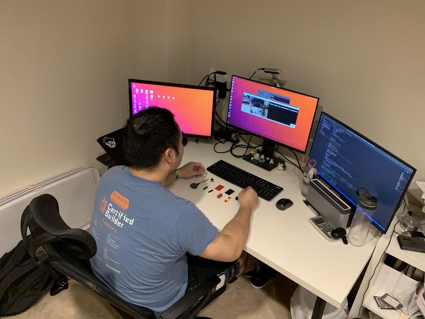
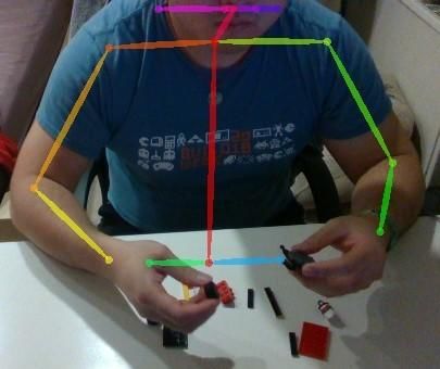
(a) Projected visualization of predicted arm motion. (b) 3D visualization of predicted arm motion. Yellow:
Yellow: shoulder joint. shoulder. Green: wrist.
Figure 1.1: Visualizations of the predicted human arm motion trajectory (10 steps) using RNNIK-
MKF. Red: current arm configuration. Black: 10-step future arm configuration.
1.1 Challenges
Human behavior is difficult to predict. One major challenge is that it is expensive to collect
a motion dataset that comprehensively covers all possible scenarios. One reason that leads
to the high cost is the diversity of the data. For example, in a human motion dataset where
the humans are doing assembly tasks, it is expensive (if not impossible) to collect data from
all human subjects in all possible task situations. However, human subjects with different
habits, body structures, moods, and task proficiencies may exhibit different motion patterns.
Failure to include sufficient data to reflect these differences will lead to poor performance
of the learned prediction model in real situations.
Another reason for the high cost of data collection is the existence of exogenous input
disturbances. For example in Fig. 1.3(b), the images captured by a camera are likely to
have black pixels not be completely black due to the inevitable sensor noise. Although these
pixel-level differences do not confuse humans, they can easily fool the image classification
models [46, 10]. Another example is shown in Fig. 1.3(c) for human motion data. Due
to the inevitable sensor noise and algorithm uncertainty, the captured motion trajectory
(red) may slightly deviate from the ground truth motion (white). These disturbances ideally
should not change the output of the prediction model, but can actually easily fool the
prediction model to make a wrong prediction if the model has not seen sufficiently many
2CHAPTER 1. INTRODUCTION
(a) Assembling. (b) Reaching. (c) Retrieving.
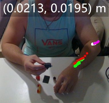
Figure 1.2: Visualizations of intention prediction. Red: predicted operation type. Green: ground-
truth operation type. White dots: observed human motion (10 steps). Red bounding boxes: usable
components. Numbers on the red bounding boxes: likelihood to be the next piece for use.
disturbed data during training. However, it is expensive (if not impossible) to generate a
full distribution of these disturbances on each data point.
Due to these high costs of data collection, a well-distributed and sufficient human
behavior dataset is usually not available. Early works [2, 22, 18, 25] have shown that an
insufficient amount of training data would make it difficult to train the neural network
(NN) model, as the performance of the learned model will deteriorate in testing. Therefore,
the learned model is not deployable in real applications. To deal with the data deficiency,
we explore methods, both online and offline, that are suitable for constructing robust NN
motion and intention prediction models.
1.2 Motion Prediction
Online adaptation is an online approach to deal with data scarcity. We propose an online
adaptable motion prediction framework (RNNIK-MKF) to predict human arm motion. In
particular, a modified Kalman filter (MKF) is used for adapting the prediction model online.
The MKF incrementally updates the prediction model using the incoming data and makes
the initially poorly trained model perform better during the runtime.
The proposed method has several advantages. First, the method is adaptable, hence
can easily and robustly generalize to unseen situations that the training data does not
cover. Many existing approaches [35, 15, 36] have been proven to work well in trained
environments, but have limited generalizability. However, it is impossible to obtain motion
data from all workers with all possible demonstrations, and comprehensively validate the
model for all situations. The proposed RNNIK-MKF enables online model adaptation
3CHAPTER 1. INTRODUCTION using MKF to achieve better generalizability with few training data. Second, the proposed structure can explicitly encode the kinematic constraints into the prediction model, which is explainable. Current approaches, such as [21], used complex graph neural network structures to encode the structural information, which is complicated and implicit. The proposed method uses the physical model derived from the human arm, which is explainable and intuitive. Thus, the predicted arm motion, as shown in Fig. 1.1, preserves the physical human arm structure. Third, the proposed method is robust when occlusion of the arm happens. Few existing methods [41] considered the situation when a partial human body is not observable. Yet the situation is common during collaboration as the robot could go between the sensor and the human arm, and thus, occluding the body part. Our method using the physical arm model can robustly predict the arm positions even when a portion of the arm, e.g., the elbow, is blocked from view. The proposed framework is tested on collected human motion data [33] with up to 2 s prediction horizon. The experiments demonstrate that the proposed method improves the prediction accuracy by approximately 14% comparing to the existing methods on seen situations. It stably adapts to unseen situations by keeping the maximum prediction error under 4 cm, which is 70% lower than other methods. Moreover, it is robust when the arm is partially occluded. The wrist prediction remains the same, while the elbow prediction has 20% less variation. 1.3 Intention Prediction We propose an iterative adversarial data augmentation (IADA) framework to train robust NN classifiers offline with limited data to tackle the data scarcity challenge in intention prediction. This framework leverages formal verification and expert guidance for iterative data augmentation during training. The key idea of IADA is that we need to find the most “confusing” samples to the NN, e.g., the samples on the decision boundary of the current NN, and add them back to the dataset. We use formal verification to find these samples by computing the closest adversaries to the existing data (called roots) in L∞ norm. These samples are called “adversaries” since the current NN predicts that they have different labels from the labels of roots (hence they are on the decision boundary of the current NN). The IADA framework will seek expert guidance to label these samples in order to ensure the correctness of adversaries. The sample is a true adversary if its ground truth label is the same as the label of its root; otherwise, this sample is a false adversary. The proposed 4
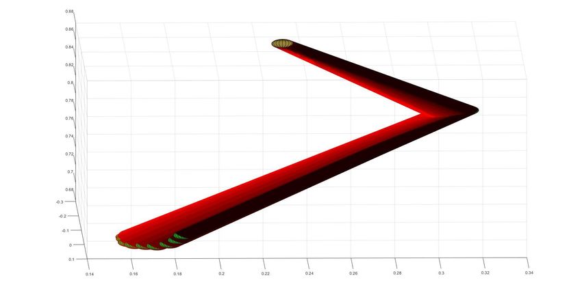
CHAPTER 1. INTRODUCTION

                          NN Decision Boundary

  2D Ground Truth                                               Digit: 2
                                                 Original
                                  ...             Image

                                                                Digit: 8

                                                 Digit: 1       Digit: 7

                                                            …              …
                            Augmented Data

                    (a)                                            (b)                   (c)
Figure 1.3: Adversarial data augmented by IADA. (a) Artificial 2D dataset. Left: Ground truth
decision boundary. Right first row: NN decision boundary. Right second row: adversarial data
augmented by formal verification and expert guidance given the current NN model. (b) MNIST
dataset. Left: original training image. Second column: the first level adversaries found around the
original image. Third column: the second level adversaries found around the first level adversarial
images. Right: further expansions. (c) Human motion dataset. White: original wrist trajectory. Red:
adversarial wrist trajectories being augmented to the training data.

IADA framework incorporates human-in-the-loop verification as the expert guidance. The
labeled samples will be added back to the training dataset no matter what labels they
are. The true adversarial samples can improve the robustness of the network, while the
false adversarial samples can help recover the ground truth decision boundary. The IADA
framework iteratively expands the dataset and trains the NN model.
    The IADA framework has several advantages. First, it is composable since it allows
easy switch of individual modules (i.e., the training algorithm, the formal verification
method, and the method for expert guidance). Second, it is safe and explainable due to
the inclusion of expert guidance, unlike other adversarial training methods. Lastly, it is
generic and appliable to general NNs, unlike existing data augmentation methods that
require strong domain knowledge. To verify the effectiveness of the IADA training, we
applied it to the human intention prediction task on a collected human motion dataset
[33]. To validate the generalizability of IADA, we applied it to two additional applications,
including a 2D artificial binary classification task as shown in Fig. 1.3(a), and the MNIST
digits classification task [28]. We compared our training framework against several existing
training methods. The results demonstrate that our training method can improve the
robustness and accuracy of the learned model from scarce training data. The IADA training
framework is suitable for constructing reliable and robust intention prediction models given
the scarce human motion dataset.
    The contributions of this thesis work can be summarized as follows:

                                                                                                 5
CHAPTER 1. INTRODUCTION
1. Constructs a human motion dataset that studies the human upper limb motion when
doing LEGO assembly tasks.
2. Proposes a novel RNNIK-MKF adaptable human arm motion prediction framework to
predict high-fidelity arm motion. We demonstrate that the RNNIK-MKF outperforms
the existing methods by showing that it can predict high-fidelity arm motion; it is
generic to unseen humans or tasks; it is more robust when partial arm motion is
occluded.
3. Proposes a novel IADA training framework that addresses the data scarcity challenge
offline during the model training phase. We demonstrate that the IADA training can
learn robust prediction models from scarce data for intention prediction.
6Chapter 2
Related Work
2.1 Human Motion Prediction
Human motion prediction has been widely studied [43]. Early approaches [14] addressed
the problem in a probabilistic way using Hidden Markov Models to estimate the possible
areas that human arms are likely to occupy. Assuming human motions are optimal, [35]
intended to learn a cost function of human behaviors by inverse optimal control and made
predictions according to the learned cost function. Recent works [26, 4] addressed the
prediction as a reaching problem by specifically learning the motion of human hands
using neural networks. The recent development of recurrent neural network (RNN) had an
outstanding performance in motion prediction [44]. The Encoder-Recurrent-Decoder (ERD)
structure [15], which transformed the joint angles to higher-dimensional features, was shown
to be effective in motion prediction. [36] added the sequence-to-sequence architecture
to address the prediction as a machine translation problem. Recently, [21, 8] devoted to
embedding the structural information of the human body into the neural networks. However,
existing methods suffer from several problems. First, neural networks are pre-trained and
fixed, which may have limited generalizability or adaptability to unseen situations. [12]
incorporates online adaptation to improve the model performance online, but it only focuses
on the single-joint motion. Second, the physical constraints of the human body are encoded
using complex neural network structures, which is unintuitive and difficult to verify.
7CHAPTER 2. RELATED WORK
2.2 Human Intention Prediction
Human intention prediction has been widely studied recently. Many works, such as [53],
focus on predicting the operation types. However, to the best of our knowledge, no existing
works have addressed the data scarcity challenge specifically in the human intention
prediction context. Nonetheless, there are approaches in other applications that address the
data scarcity challenge.
2.2.1 Data Augmentation
Learning from insufficient training data has been widely studied [2, 22, 18, 25]. Data
augmentation (DA) is a widely used approach. People use different approaches to gener-
ate additional data given the existing dataset [45] to improve the generalizability of the
classifiers. [55, 13] propose either to manually design a policy or search for an optimal
policy among the pre-defined policies to generate new data. On the other hand, instead
of explicitly designing the policy, [40, 29, 3, 7] propose to learn generative NN models to
create new data. However, manually designing the augmentation policy requires strong
domain knowledge. In addition, the designed policy might only be suitable for a small
range of related tasks. On the other hand, using NNs (GANs) for DA is knowledge-free.
However, it has poor explainability, which might be a potential concern for safety-critical
tasks.
2.2.2 Adversarial Training
Adversarial training [5] is a widely used approach for improving the NN model robustness.
It has been widely studied since [46] first introduced the adversarial instability of NNs.
Given the existing training data D0 , the adversarial training objective is formulated as a
minimax problem,
min E(xi ,yi )∈D0 max L( fθ (xi + δi ), yi ), (2.1)
θ ||δi ||∞ ≤ε
where δi is the adversarial perturbation and ε is the maximum allowable perturbation.
Early works [46, 16] efficiently estimate the adversarial perturbations based on the gradient
direction. However, [38] showed that the estimation in the gradient direction might be
8CHAPTER 2. RELATED WORK
inaccurate, and thus, makes the trained model sub-optimal. Recent work [11] proposes to
adaptively adjust the adversarial step size during the learning process. Based on the idea
of curriculum learning, [54] propose to replace the traditional inner maximization with a
minimization, which finds the adversarial data that minimizes the loss but has different
labels. The adversarial data generated via minimization is also known as the friendly
adversarial data. On the other hand, neural network verification provides a provably safe
way to find the adversarial samples with minimum perturbations, which are the most friendly
adversaries. In fact, many works on neural network verification [38, 6, 47] have shown
that using the adversarial samples from verification is effective for adversarial training.
However, these methods might incorrectly take false adversaries as true adversaries, which
might adversely harm the model training. Moreover, they only improve the local robustness
of the trained model around the training data, and thus, have limited capacity to improve
the generalizability of the network in real situations.
9CHAPTER 2. RELATED WORK 10
Chapter 3
Problem Formulation
3.1 Motion Prediction Formulation
The motion prediction in this thesis tackles the skeleton motion prediction problem on
production lines, where humans collaborate with robot arms in confined workspaces. In
these environments, the trunk of the human body tends to stay still and the major body
parts interacting with the robot are the human arms. Therefore, we focus on predicting
human arm motion, including the elbow and the wrist, as shown in Fig. 3.1. Note that the
motion prediction is a regression problem, in which the prediction model maps the N-step
historical arm motion observation to the future M-step arm motion.
In the motion prediction context, this thesis uses regular symbols and ∧ to denote the
observation and prediction respectively. The wrist and elbow positions at time k are denoted
as wk , ek ∈ R3 . The position vector p ∈ R6 is constructed by stacking the positions of the
wrist and elbow. We define the observation and prediction at time k as
pk−N+1 p̂k1
k
... p̂2
∈ R6N , 6M
xk = ... ∈ R .
ŷk = (3.1)
p
k−1
pk p̂kM
The constants M, N ∈ N are the prediction and observation horizons. p̂kj is the jth step
prediction at time k. We need to build a prediction model, ŷk = f (xk ), that predicts the
future skeleton motion.
11CHAPTER 3. PROBLEM FORMULATION
ê 1k ê 2k ê Mk
k
…
ŵ2
ŵ 1k ŵ Mk
M-step
Arm Motion Future Trajectory
Prediction
N-step
Historical Trajectory Arm Model
ek-N+1 ek-N+2 … ek
wk-N+1 wk-N+2 wk
Time
Figure 3.1: Illustration of the arm motion prediction problem. The problem takes in the N-step
historical arm trajectory and outputs the M-step future arm trajectory. The human arm is modeled as
a 5-DOF manipulator.
However, due to the data scarcity in the human motion dataset, the learned model
f , which is validated in the training environment, would be less accurate and has poor
generalizability in real situations. Therefore, we use online adaptation to address the data
scarcity challenge in motion prediction. The goal is to construct an adaptable model,
ŷk = f (xk , ŷk−1 ), which is a time-varying function. The model f takes in the observed
N-step historical trajectory and the previous M-step prediction and outputs the M-step
future trajectory. The adaptation algorithm adjusts the model online and improves the
generalizability.
12CHAPTER 3. PROBLEM FORMULATION
3.2 Intention Prediction Formulation
Human intention prediction predicts the intention labels that describe the human behavior
as shown in Fig. 3.2. Note that the intention prediction is a classification problem, in which
the model maps the input, including the N-step historical arm motion observation and the
environment information, to the corresponding pre-defined intention labels as shown in
Fig. 3.2.
At timestep k, the prediction model is given with the N-step observation of the human
motion and the environment information as
wk−N+1 pc1
w
... 6N
... 3K
∈ R , env =
xk = pc ∈ R , (3.2)
w
k−1 K−1
wk pcK
where K denotes the number of possible components and pci ∈ R3 denotes the position of the
workpiece i. The prediction model outputs the intention label y, including 1) the operation
type and 2) the next assembly step. In our intention prediction case, the operation type
has four different labels as shown in Fig. 3.2, including assembling, retrieving, reaching,
and abnormal. The next assembly step has K different labels, corresponding to all possible
components. Therefore, the intention prediction model can be written as yk = f (xkw , envi ).
However, due to data scarcity, it is difficult to learn a robust and accurate f by merely
designing sophisticated NN structures. Therefore, we use a standard fully-connected neural
network (FCNN) to construct the prediction model f since it is decently powerful to model
arbitrary nonlinear functions. Then, the major problem becomes how to learn a robust and
accurate f given the insufficient human motion dataset.
Given a training dataset D0 = {(xi , yi )}ni=1 where x is the input and y is the output label,
the regular supervised training learns the NN model by solving the following optimization
1
min Σni=1 L( fθ (xi ), yi ) =: E(xi ,yi )∈D0 L( fθ (xi ), yi ) ,
(3.3)
θ n
where L is the loss function, θ is the NN model parameter, and fθ is the NN transfer
function. Our goal is to learn a model that minimizes the expected loss when deployed in
13CHAPTER 3. PROBLEM FORMULATION
Assembling
Environment Retrieving
Intention Label: Reaching
Abnormal
Intention Next wanted piece: X
Prediction
N-step
Historical Trajectory
ek-N+1 ek-N+2 … ek
wk-N+1 wk-N+2 wk
Time
Figure 3.2: Illustration of the intention prediction problem. The problem takes in the N-step motion
observation and outputs the corresponding pre-defined intention labels.
real applications:
min E(x,y)∈D (L( fθ (x), y)), (3.4)
θ
where D represents the real input-output data distribution, which is unavailable during
training. When D0 is similar to D, we can obtain a fθ that behaves similarly as the ground
truth f . However, in our case (i.e., behavior/intention prediction), D0 is insufficient, and
thus, leading to a poorly trained fθ that behaves differently as f . The goal is to learn a
robust and accurate f offline given the insufficient human motion dataset.
14Chapter 4
Approach
4.1 RNNIK-MKF Motion Prediction
In general assembly tasks, humans move their hands with clear intention while the elbows
are mainly to support the hand motion. Hence, we separate the motion prediction problem
into wrist motion prediction and arm motion prediction. We use a recurrent neural network
(RNN) for modeling the complex wrist motion and inverse kinematics (IK) to encode
the physical body constraints and extend the wrist prediction to full-arm prediction. The
modified Kalman filter (MKF) is used for online adapting the model to different humans
and tasks and addressing the data scarcity challenge in human motion prediction. The
proposed RNNIK-MKF framework is shown in Fig. 4.1.
4.1.1 RNN for Wrist Motion Prediction
Human wrist motion is complex and highly nonlinear. In addition, human motion has strong
temporal connections. Therefore, we choose RNN since it is powerful to model arbitrary
nonlinear functions and has hidden states to memorize past information. In particular, the
Long Short-term Memory (LSTM) cell [19] is used since it has adequate gates to control
the memory either to remember or to forget. We use an N-to-1 structure [15], where the
RNN takes in the N-step wrist history and outputs the next single step wrist prediction
as shown in Fig. 4.1. For an M-step prediction, the network iteratively appends the new
prediction to the input and then predicts for the next step, until the M-step prediction is
obtained as shown in Eq. (4.3). The structure has the advantage to enable more flexibility
15CHAPTER 4. APPROACH
Prediction: ŷk-1 ŷk ŷk+1
ê 1k ê 2k ê Mk
MKF IK IK IK
ŵ 1k ŵ 2k
... ŵ Mk
-
MKF Linear Linear Linear
RNN
LSTM LSTM LSTM
Observation: xk-1 xk xk+1
Figure 4.1: RNNIK-MKF motion prediction framework.
on the online adaptation since we can adapt the model as soon as a new observation is
available.
We use LST M and RNN to denote the transition of a single LSTM cell and the N-to-1
prediction respectively. Given the N-step historical wrist trajectory at time k, the hidden
states of the LSTM cells are propagated as
[h1 , c1 ] = LST M(wk−N+1 , 0, 0),
[h2 , c2 ] = LST M(wk−N+2 , h1 , c1 ),
(4.1)
...
[hN , cN ] = LST M(wk , hN−1 , cN−1 ).
The first step wrist prediction is obtained using a linear layer
ŵk1 = φk hN + bl , (4.2)
where φk is the adaptable weight matrix (discussed in section 4.1.3) of the linear layer at
time k and bl is a constant bias. The LSTM cells Eq. (4.1) and the linear layer Eq. (4.2)
16CHAPTER 4. APPROACH
construct the N-to-1 RNN. We solve the prediction problem as
ŵk1 = RNN(φk , [wk−N+1 , ..., wk ]T ),
ŵk2 = RNN(φk , [wk−N+2 , ..., wk , ŵk1 ]T ), (4.3)
...
until M-step wrist prediction is obtained.
4.1.2 IK for Arm Motion Prediction
The arm motion is mainly supporting the wrist motion, and thus, has a relatively simple
motion pattern. Therefore, we use the model-based IK to model the arm motion. A general
human arm can be decomposed into a 5-DOF manipulator as shown in Fig. 3.1. The
shoulder is decomposed into 3 revolute joints and the elbow is decomposed into 2 revolute
joints. The wrist is considered as the end-effector. The state of the arm in the joint space is
θ ∈ R5 . The end-effector state is w ∈ R3 . The IK problem solves for θ̂ under the predicted
wrist position ŵ where θ̂ = IK(ŵ | θ , w), given the current states θ and w. A popular
approach to solve the IK problem is using the Jacobian [50]. The Jacobian J(θ ) ∈ R3×n for
an n-DOF robot manipulator is
∂ IK(w) −1
∂ FK(θ )
J(θ ) = ≈ , (4.4)
∂θ ∂w
where FK(θ ) : Rn → R3 is the forward kinematics. Using matrix transpose to replace
matrix inverse, we can solve the IK problem as
θ̂ = θ + AJ(θ )T (ŵ − w), (4.5)
where A ∈ Rn×n is an adaptable parameter matrix (discussed in section 4.1.3) that encodes
the individual differences on the joint velocities, e.g., some workers tend to place the elbow
on the table, while others prefer to move with the wrist. We can solve the arm prediction by
solving the IK for each predicted wrist position.
17CHAPTER 4. APPROACH
Algorithm 1 Modified Kalman Filter
1: Input: MKF parameters: λ > 0, σw ≥ 0, σv ≥ 0.
2: Input: EMA parameters: 0 ≤ µv < 1, 0 ≤ µ p < 1.
3: Input: Φk−1 , Ek = (yk−1 − ŷk−1 ), Xk−1 .
4: Output: Φk .
5: Internal State: Z, V .
K = Zk−1 Xk−1T (X T −1
6: k−1 Zk−1 Xk−1 + σw I)
7: Vk = µvVk−1 + (1 − µv )KEk
8: Φk = Φk−1 +Vk
9: Z ∗ = λ1 (Zk−1 − KXk−1 Zk−1 + σu I)
10: Zk = µ p Zk−1 + (1 − µ p )Z ∗
4.1.3 Online Adaptation with MKF
Human motion is diverse and time-varying. For instance, a worker might initially move the
entire arm. But after a while, the worker would probably rest the elbow on the table and only
move the wrist. Moreover, different individuals can perform the same task very differently
due to different body structures or task proficiency. It is expensive (if not impossible) to
collect a dataset that comprehensively includes all possible situations. Therefore, the data
we use for training is highly likely to be scarce and insufficient. Due to the data scarcity, the
learned prediction model might deviate from the true prediction model, and thus, perform
poorly during testing or deployment. Therefore, online adaptation is important to make
the method robust and generic to unseen situations. In the proposed framework, the wrist
predictor has a linear output layer Eq. (4.2) in φ , and the arm predictor Eq. (4.5) is linear in
A. Therefore, we apply linear adaptation to the system.
Many existing online adaptation algorithms are based on stochastic gradients [23].
However, these methods have no guarantee of optimality. Thus, we use a second-order
method in order to achieve better convergence and optimality. Recursive least-squares
parameter adaptation algorithm (RLS-PAA) [17] is an optimal method. However, since
the regular RLS-PAA does not consider a noise model of the system, it is inefficient
to tune. In addition, we need to apply smoothing techniques to the internal adaptation
parameters to ensure stable adaptation and prediction under noisy measurements. Moreover,
we want the more recent information to have more impact on the current estimation. Hence,
we propose to use MKF for online adaptation. We add a forgetting factor, λ , to the
conventional Kalman filter to prevent the estimation from saturation. In addition, we apply
18CHAPTER 4. APPROACH
the Exponential Moving Average (EMA) filtering method discussed in [1] to smooth the
adaptation process.
The linear prediction system can be written as
Φk = Φk−1 + ωk ,
(4.6)
ŷk = Φk Xk + vk .
For wrist prediction, ŷ is the wrist prediction. Φ and X are the parameter matrix φ and
hidden feature hN in Eq. (4.2). For arm prediction, ŷ is the arm prediction, Φ and X are
equivalent to A and J(θ )T (ŵ − w) in Eq. (4.5). ωk ∼ N(0, σw ) and vk ∼ N(0, σv ) are virtual
Gaussian white noises. The MKF adaptation algorithm is summarized in algorithm 1. There
are two internal variables: the covariance matrix Z and the parameter update step V . The
learning gain, K, is calculated on line 6 using the Kalman filter’s formula. V is calculated
using the EMA filtering on line 7. The parameter matrix Φ is updated on line 8. Then Z is
updated using the forgetting factor on line 9 and then smoothed using EMA on line 10.
Following the approach in [12] that applies RLS-PAA to the linear output layer of a
fully connected neural network (FCNN), we apply the MKF to Eq. (4.2) with respect to
φ as well as to Eq. (4.5) with respect to A. The virtual noises ω and v are tunable in the
adaptation.
The proposed RNNIK-MKF framework is then summarized in algorithm 2. MKF
denotes the adaptation in algorithm 1. The superscripts w and a distinguish the variables
for wrist and arm predictions. FKew = [FK; FKe ] where FK and FKe are the forward
kinematics to wrist and elbow. IKew solves for the arm state θ pre when both wrist and elbow
positions are known. For each time step, the algorithm obtains the current configuration in
line 6. The parameters are updated using MKF on lines 11, 13. If occlusion happens, the
adaptation is turned off on line 16. Then the algorithm iteratively predicts the future wrist
and elbow trajectories for M steps on lines 20 and 22.
4.1.4 Online Adaptation Estimation Error Propagation
As the MKF consistently adjusts the model parameters online, the performance of the
prediction model varies as time changes. It is important to quantify the error of the
motion prediction as the adaptation proceeds. Given the prediction system in Eq. (4.6),
the uncertainty of the prediction by RNNIK-MKF can be quantified by 1) the statistical
19CHAPTER 4. APPROACH
Algorithm 2 RNNIK-MKF Motion Prediction
1: Input: Pre-trained RNN, Arm Model, φ0 = φtrained , A = I.
2: Input: MKF parameters: 0 < λ w ≤ 1, σww ≥ 0, σvw ≥ 0, 0 < λ a ≤ 1, σwa > 0, σva ≥ 0.
3: Input: EMA parameters: µvw , µ pw , µva , µ pa ∈ [0, 1).
4: Output: Full arm trajectory prediction ŷ
5: for i = 1, 2, . . . , k do
6: Obtain current configuration wi , ei .
7: xiw = [wi−N+1 ; . . . ; wi−1 ; wi ], w pre = wi .
8: for j = 1, 2, . . . , M do
9: if j = 1 then
10: if Observation Available then
11: φi = MKF(φi−1 , wi − ŵi−1 1 , hi−1 )
a = JT (θ )(w −
12: Xi−1 i−1 i wi−1 )
13: Ai = MKF(Ai−1 , θi − θ̂1i−1 , Xi−1 a )
14: θ pre = IKew ([wi ; ei ])
15: else
16: φi = φi−1 , Ai = Ai−1
17: θ pre = IKew ([wi ; êi−1 1 ])
18: end if
19: end if
20: ŵij = RNN(φi , xiw )
21: xiw = [wi−N+ j ; . . . ; wi ; . . . ; ŵij ]
22: θ̂ ji = θ pre + Ai J(θ pre )T (ŵij − w pre )
23: [w pre ; êij ] = FKew (θ̂ ji ), θ pre = θ̂ ji
24: end for
25: ŷi = [ŵi1 ; êi1 ; . . . ; ŵiM ; êiM ]
26: end for
standard deviation of the prediction error and 2) the propagation of the mean squared
estimation error (MSEE) [30].
Statistical standard deviation At timestep k, the prediction error is calculated as ek =
yk − ŷk . The statistical standard deviation of the prediction error is calculated as
s s
∑T1 e2k ∑T1 (yk − ŷk )2
σy = = , (4.7)
T T
where T is the total prediction timesteps.
20CHAPTER 4. APPROACH
Propagation of a priori MSEE As illustrated in algorithm 1, the covariance matrix, Zk ,
propagates and is the MSEE of the model parameters during online adaptation. Given the
covariance matrix Zk at time step k, the covariance matrix of the motion prediction ŷk can
by calculated as
Zkŷ = Φk Zk ΦTk + vk , (4.8)
where vk is the Gaussian noise and Φk is the parameter matrix being adapted as illustrated
in Eq. (4.6). And Zkŷ is the a priori MSEE of the prediction ŷk and quantifies the prediction
uncertainty error.
21CHAPTER 4. APPROACH
4.2 IADA Intention Prediction
Due to the data scarcity, a standard fully-connected neural network (FCNN) classifier can
achieve outstanding performance on the training data but fails to perform well on the testing
data or real deployment. To address the challenge, we aim to augment the insufficient
dataset D0 with adversarial data Dadv to robustly learn the true decision boundaries of the
real but unknown data D as discussed in section 3.2. The goal is to ensure the learned
model on D0 ∪ Dadv is as close as possible to Eq. (3.4). To achieve the goal, we formulate
the training problem as a two-layer optimization
min E(x,y)∈D0 ∪Dadv (L( fθ (x), y)),
θ
n o
Dadv = x0 , label(x0 ) | ∃(x0 , y0 ) ∈ D0 , x0 = arg minx0 s.t. ||x0 −x0 ||∞ ≤ε∧ fθ (x0 )6=y0 L0 ( fθ (x0 ), y0 ) .
(4.9)
The outer objective optimizes the NN model parameters θ to minimize the loss on the data
from D0 ∪ Dadv . The inner objective constructs Dadv given θ , which essentially finds the
most friendly adversarial data for all training data. The most friendly adversarial data for
(x0 , y0 ) ∈ D0 is an input sample x0 that is at most ε distance away from x0 in the L∞ norm
but changes the network output from y0 with the smallest loss L0 . The loss L0 for the inner
objective may or may not be the same as the original loss L. Ideally, we should choose
a loss that guides us to the most “confusing” part of the input space. The label of these
friendly adversarial data is decided by an additional labeling function, which ideally should
match the ground truth. If label(x0 ) = y0 , we call x0 a true adversary; otherwise a false
adversary.
We propose an iterative adversarial data augmentation (IADA) training framework to
solve Eq. (4.9). Figure 4.2 illustrates the proposed training framework that aims to solve
the problem defined in Eq. (4.9). In particular, the inner objective will be solved using
formal verification to be discussed in section 4.2.1, while the labeling will be performed
under expert guidance to be discussed in section 4.2.2. The iterative approach to solve the
two-layer optimization will be discussed in section 4.2.3.
22CHAPTER 4. APPROACH
Dataset Augment data with unverified labels Expert Guidance
Network Training
Scheduler
(Whether to
ask for human
Adversarial
verification of
Data the label)
Trained Network
Formal Verification Human
Verification
Training (labeling the
Data data)
Augment data with verified labels
Figure 4.2: Iterative Adversarial Data Augmentation (IADA) training framework. For (x, y) ∈
D0 ∪ Dadv , the framework updates the model. If (x0 , y0 ) ∈ D0 , the formal verification finds the most
friendly adversarial sample x0 around x0 if exists. The scheduler determines if human verification is
required for x0 . If not, (x0 , y0 ) is augmented to Dadv . Otherwise, if human is able to assign y0 , then
(x0 , y0 ) is added to D0 . If not, then (x0 , y0 ) is appended to Dadv .
4.2.1 Formal Verification to Find Adversaries
The two-layer optimization in Eq. (4.9) is similar to the formulation of adversarial training
Eq. (2.1). The major distinction lies in the inner objective. The minimax formulation
in Eq. (2.1) might reduce the model accuracy and generalizability when maximizing the
robustness [48] since the inner maximization could be too aggressive when generating
adversaries. Similar to the approach in [54], instead of finding the adversaries via the inner
maximization, we take the adversarial label fθ (x0 + δ0 ) into consideration when generating
the adversarial sample x0 = x0 + δ0 . In particular, we design the inner loss to penalize the
magnitude of δ0 . Then the inner optimization in Eq. (4.9) can be written as
min
0
kx0 − x0 k∞ , s.t. kx0 − x0 k∞ ≤ ε, fθ (x0 ) 6= fθ (x0 ). (4.10)
x
The reason why we use the distance metric in the input space as the loss L0 instead of
using the original loss or any other loss that penalizes the output is that this metric reflects
the “confusing” level of samples. We generally expect that the learned model is regular
23CHAPTER 4. APPROACH at the training data for generalizability. The easier it is to change the label by perturbing the input data, the less regular the model is, and hence more “confusing”. In addition, this formulation provides a quantitative metric δ0 for evaluating the robustness online. Therefore, we can prioritize enhancing the weaker boundaries and obtain full control of the training process. Nevertheless, the optimization in Eq. (4.10) is nontrivial to solve due to the nonlinear and nonconvex constraints introduced by fθ . To obtain a feasible and optimal solution, we use formal verification [32] to find the appropriate x0 . The optimization in Eq. (4.10) essentially finds the minimum input adversarial bound, which can be solved by various neural verification algorithms. In particular, primal optimization- based methods such as MIPVerify [47] and NSVerify [34] solve the problem exactly by encoding the neural network into a mixed-integer linear program; dual optimization-based methods [52] can compute an upper bound of the problem by relaxing the nonlinear ReLU activation functions; reachability-based methods [51] can also compute an upper bound by over-approximating the reachable set and binary search for the optimal loss. 4.2.2 Expert Guidance for Labeling With the adversaries obtained from formal verification, we need to label them before augmentation. The proposed IADA framework uses expert guidance to guarantee the safety and accuracy of the training. The framework requires the human expert to verify the newly added adversaries. It uses a scheduler to balance the required human effort and the training accuracy. We use an ensemble NN and the L∞ distance check to construct the scheduler. The ensemble NN indicates whether the adversary is meaningful. We say data is meaningful if humans can properly interpret the data label. For example, the disturbance to a human trajectory that violates human kinematic constraints or to MNIST images that have two digits shown in one image is not meaningful. However, note that it is difficult to obtain an accurate ensemble model that can filter out all unmeaningful adversaries. However, it is tolerable since the framework keeps two datasets, D0 and Dadv discussed in section 4.2.3, although the human expert might have extra work to do, which is more than needed. The scheduler requires human verification if δ0 > d or the ensemble model agrees that the adversary is meaningful, where d is a pre-defined threshold. Based on the application, a smaller d can be chosen to require more frequent human verification to improve the training accuracy, while a larger d alleviates the amount of human effort. 24
CHAPTER 4. APPROACH

4.2.3    Iterative Adversarial Data Augmentation
We use an iterative approach to solve the two-layer optimization in Eq. (4.9) by incremen-
tally augmenting the data with the outer NN training loop. In one iteration, we find the
adversaries generated in section 4.2.1, which are the most “confusing” points for the current
NN. The adversaries will be labeled by experts and augmented to the dataset, either D0 or
Dadv , as shown in Fig. 4.2. In the next iteration, the framework will further verify, label, and
expand the dataset based on the augmented dataset. The framework maintains two datasets
D0 and Dadv , where Dadv is initially empty and D0 starts with the original training data. The
adversaries are only augmented to D0 if they are verified by the human expert, otherwise,
they are pushed into Dadv . Note that the adversaries generated in section 4.2.1 can either be
true or false adversaries, but both are informative and useful for improving the NN learning.
However, incorrectly mixing these two types of adversaries can greatly harm NN learning.
Therefore, we maintain D0 and Dadv to distinguish the safe data and potentially incorrect
data. The framework iteratively expands only from the data (x0 , y0 ) ∈ D0 . Therefore, the
framework can further expand the available training data safely. Dadv will be refreshed
before verification as shown in algorithm 3, since the framework only wants temporary
effect from Dadv but permanent effect from D0 for safety and correctness. Also note that
the IADA framework is reduced to standard adversarial training, except that we have a
different inner minimization loss objective if the scheduler requires no human verification.
On the other hand, it is equivalent to standard online data augmentation when the scheduler
always requires human verification (similar to data aggregation in imitation learning [42]).
Based on the applications, the scheduler can be tuned to either require more or less expert
knowledge to balance the training accuracy and the human effort.
    The IADA framework is summarized in algorithm 3. The verification rate rv indicates
the frequency of online formal verification and data augmentation. The verification number
C indicates a maximum number of points to verify at each iteration. Qv is a priority queue
based on the level of expansion and the perturbation bound δ . The level is defined as 0
for the original training data. The adversaries generated from the original data have level
1. Qv determines the weakest points and prioritizes those points during verification and
expansion. On line 12, the system gets the weakest point and verifies it on line 14. If the
robustness is not satisfied, the system either asks for expert knowledge to assign a label
or assumes it to have the same label as the root. If the label is assigned by humans, the

                                                                                             25
CHAPTER 4. APPROACH
Algorithm 3 Iterative Adversarial Data Augmentation (IADA)
1: Input: Original dataset (x0 , y0 ) ∈ D0 .
2: Input: Robustness bound ε, verify rate rv , verification number C, learning rate α.
3: Output: NN parameter θ .
4: Initialize: θ = θ0 , Qv = {D0 }.
5: repeat
6: if VerificationRound(rv ) then
7: // Refresh Dadv since it might contains data with incorrect labels.
8: Clear Dadv .
9: for i = 1, . . . ,C do
10: Breaks if Qv is empty.
11: // Qv prioritizes the point with 1) the lowest level of expansion and 2) the smallest
perturbation bound.
12: (x, y) = Qv .pop.
13: // Find an adversary by solving Eq. (4.10).
14: x0 = Veri f y(θ , x, y, ε).
15: Skip if no adversary x0 is found.
16: if Scheduler && Human Verified then
17: Obtain the verified label y0 .
18: Push (x, y) and (x0 , y0 ) to Qv and append (x0 , y0 ) to D0 .
19: else
20: Append (x0 , y) to Dadv .
21: end if
22: end for
23: end if
24: for minibatch {X,Y } in D0 ∪ Dadv do
25: θ ←− θ − αL( fθ (X),Y ).
26: end for
27: until max_epoch reached.
28: return θ .
adversarial sample is added to D0 for further expansion. The NN model is updated using
the training data and the adversarial data at lines 24-26.
4.2.4 Prediction Confidence Estimation
The prediction model outputs the corresponding classification labels. However, it is possible
that the output label is incorrect. Mistakenly trusting the incorrect prediction would harm
the downstream modules and potentially lead to safety hazards. Therefore, it is important
to estimate the reliability of the prediction. We use a confidence value to quantitatively
26CHAPTER 4. APPROACH
estimate the reliability of the prediction. Ideally, it is desired that the correct predictions
have higher confidence and incorrect predictions have lower confidence. And we can use
the confidence value to distinguish the correct and incorrect predictions.
Assuming uncertainty exists in the input x (e.g., the noise when capturing the human
motion trajectories), the uncertainty of x can be modeled as a Gaussian white noise as X ∼
N(0, σX ). We use the perturbation bound for estimating the prediction confidence. Given a
learned NN classifier, it is expected that the prediction closer to the decision boundary is
more likely to be uncertain. Therefore, we can estimate the prediction confidence C as
C = P(|t| ≤ δ ) = P(t ≤ δ ) − P(t ≤ −δ )
Z −δ
1 δ t2 1 t2
Z
=√ e− 2 dt − √ e− 2 dt (4.11)
2π −∞ 2π −∞
1
Z δ 2
t
=√ e− 2 dt,
2π −δ
where P is the cumulative distribution function of X ∼ N(0, σX ) and δ = ||x − x0 ||∞ is the
perturbation bound by solving Eq. (4.10).
Note that the confidence estimation in Eq. (4.11) is generic and can be applied in
different applications and NN models. However, the quality of the learned NN determines
if the metric is valid. This metric would be more informative and reliable for NN models
with decision boundaries closer to the ground-truth decision boundaries. This metric is
valid and informative here since the prediction model learned by IADA is close to the true
prediction model.
4.2.5 IADA Analysis
The IADA framework is unique in several ways. First, it is well-known that there exists
a trade-off between accuracy and robustness in general adversarial training [48]. This is
mainly due to incorrectly mixing the true and false adversaries. However, by introducing
expert guidance, the true adversaries can improve the NN robustness and enlarges the
decision area, while the false adversaries can enhance the ground truth decision boundary
for better accuracy. Second, although the augmented data may not recover the ground
truth data distribution, the augmented data will converge to and fully cover the ground
truth decision boundary in the limit (proof left for future work). As a result, the learned
27CHAPTER 4. APPROACH
NN will converge to the ground truth with the correct decision boundary. Hence, this data
augmentation is most effective.
Based on these features, we argue that IADA is most suitable for tasks that have non-
trivial distribution of the data around the decision boundary, such as human intention
prediction in section 5.3.4. Such tasks generally have false adversaries close to the training
data and can easily have “confused” decision boundaries. On the other hand, image-related
tasks, such as MNIST, are suitable for using IADA, but not necessarily required. It is mainly
due to that image data is generally easier to collect, thus, unlikely to have insufficient data.
In addition, it is rare to have false adversaries close to the original images.
28Chapter 5
Experiments
5.1 Data Collection
This work considers the situation on production lines, where the human worker sits in front
of a desk; and we mainly predict the human behavior based on the upper body motion. To
the best of our knowledge, such a human motion dataset that focuses on human arm motion
does not exist publicly. Therefore, we collected our human motion dataset in order to test
and validate the proposed human motion prediction and intention prediction methods.
Figure 5.1 demonstrates the experiment setup for collecting the motion data. In order to
simulate the situation in typical HRC production lines, we have humans sitting in front of a
desk doing assembly tasks using LEGO pieces. A motion capture sensor, an Intel RealSense
D415 camera, faces downward to record the human upper limb motion at approximately
30Hz. A visualizer displayed on the screen in front of the human guides the human subjects
to walk through the data collection experiment. The experiments have 3 humans doing 5
assembly tasks for 3 trials each. There are 8 available LEGO pieces provided on the desk.
Each assembly task requires 4 LEGO pieces. For each trial, the human is given the pictures
of the desired assembled object by the visualizer and then uses the provided LECO pieces
to assemble the target object based on their interpretation. The recorded data durations of
the tasks vary from 30 s to 90 s based on the task proficiency of the human subjects. The
OpenPose [9] is used to extract the human pose as shown in Fig. 3.1. Figure 5.2 shows the
example image frames of the collected motion data. The collected human motion dataset
includes the following typical operations, including
29CHAPTER 5. EXPERIMENTS
Visualizer Camera
Figure 5.1: Data collection experiment setup.
1. Assembling: the human assembles two LEGO pieces together in place Fig. 5.2(a).
2. Reaching: the human moves the wrist toward the intended LEGO piece on the desk
Fig. 5.2(b).
3. Retrieving: the human grabs the LEGO piece and moves the wrist back to the
assembling area Fig. 5.2(c).
However, due to individual differences (i.e., task proficiency, arm length, etc), the behaviors
are very different in terms of displacement and duration. Note that even though the
collected dataset includes different humans doing different assembly tasks for several trials,
the demonstrations by human subjects are far from sufficient. It is highly possible that
the test set includes motion patterns that never exist in the training set. Therefore, the
adaptability of RNNIK-MKF and the robust learning by IADA are critical to building robust
motion and intention prediction models.
5.2 RNNIK-MKF Motion Prediction
We use the motion data in section 5.1 to evaluate the proposed RNNIK-MKF motion
prediction framework. We compare our method to several existing methods, including
FCNN, FCNN with RLS-PAA (NN-RLS) [12], ERD [15], and LSTM-3LR [15]. The
proposed RNNIK-MKF has one recurrent layer with 128 hidden size. To establish a fair
30You can also read