Device quantization policy in variation aware in memory computing design
←
→
Page content transcription
If your browser does not render page correctly, please read the page content below

www.nature.com/scientificreports
OPEN Device quantization policy
in variation‑aware in‑memory
computing design
Chih‑Cheng Chang, Shao‑Tzu Li, Tong‑Lin Pan, Chia‑Ming Tsai, I‑Ting Wang,
Tian‑Sheuan Chang & Tuo‑Hung Hou*
Device quantization of in-memory computing (IMC) that considers the non-negligible variation
and finite dynamic range of practical memory technology is investigated, aiming for quantitatively
co-optimizing system performance on accuracy, power, and area. Architecture- and algorithm-level
solutions are taken into consideration. Weight-separate mapping, VGG-like algorithm, multiple cells
per weight, and fine-tuning of the classifier layer are effective for suppressing inference accuracy
loss due to variation and allow for the lowest possible weight precision to improve area and energy
efficiency. Higher priority should be given to developing low-conductance and low-variability memory
devices that are essential for energy and area-efficiency IMC whereas low bit precision (< 3b) and
memory window (< 10) are less concerned.
Deep neural networks (DNNs) have achieved numerous remarkable breakthroughs in applications such as pat-
tern recognition, speech recognition, object detection, etc. However, traditional processor-centric von-Neumann
architectures are limited in energy efficiency for computing contemporary DNNs with rapidly increased data,
model size, and computational load. Data-centric in-memory computing (IMC) is regarded as a strong contender
among various post von-Neumann architectures for reducing data movement between the computing unit and
memories for accelerating D NNs1,2. Furthermore, quantized neural networks (QNNs) that truncate weights and
activations of DNNs have been proposed to further improve the hardware efficiency3. Compared with the generic
DNNs using floating-point weights and activations, QNNs demonstrate not only substantial speedup but also a
tremendous reduction in chip area and p ower4. These are accomplished with nearly no or minor accuracy degra-
dation in the inference tasks of complex CIFAR-10 or ImageNet data3. While the emergence of QNNs opens up
the opportunity of implementing IMC using emerging non-volatile memory (NVM), the practical implementa-
tion is largely impeded by the imperfect memory characteristics, in particular, only a limited number of quantized
memory (weight) states is available at the presence of intrinsic device variation. The intrinsic device variation
of emerging NVM such as P CM5, RRAM6, MRAM7, leads to a significant degradation in inference accuracy.
Number of studies have investigated these critical issues with the focus on the impact of the DNN inference
accuracy7–9. NV-BNN focused on the impact of binary weight variation on inference accuracy, but the consid-
erations on multi-bit weights and the impact on energy and area efficiency are l acking7. Yang et al. evaluated the
impact of DNN inference accuracy based on various state-of-the-art DNNs8. The major focus was on the impact
of noise of input and weight while considering hardware efficiency. Yan et al. discussed the energy/area efficiency
and the impact of device non-ideality on inference accuracy separately but not s imultanously9. Therefore, a com-
prehensive and quantitative study that links the critical device-level specs, namely quantization policy, memory
dynamic range, and variability with those system-level specs, namely power, performance (accuracy), and area
(PPA), is still lacking. This paper intends to provide a useful guide on NVM technology choice for quantized
weights considering the variation-aware IMC PPA co-optimization. Different from the previous works, our evalu-
ation takes into account practical IMC design options at the architecture, algorithm, device, and circuit levels.
First, we compare the inherent immunity against device variation among different IMC mapping schemes. Then,
the dependence of variation immunity on DNN algorithms, quantization methods, weight precision, and device
dynamic range are discussed. To further improve the immunity against variation, the strategies of using multiple
cells to represent a higher-precision weight and fine-tuning last fully-connect classifier layer in the network are
detailed. Finally, taking into account other circuit-level constraints, such as limited current summing capability
and peripheral circuit overhead, the energy and area efficiency of variation-aware IMC designs are compared to
provide a useful guideline for future IMC PPA co-optimization.
Department of Electronics Engineering and Institute of Electronics, National Yang Ming Chiao Tung University,
Hsinchu 300, Taiwan. *email: thhou@mail.nctu.edu.tw
Scientific Reports | (2022) 12:112 | https://doi.org/10.1038/s41598-021-04159-x 1
Vol.:(0123456789)
www.nature.com/scientificreports/
Figure 1. DNN-IMC mapping schemes. (a) Naïve IMC with ± weight and + input. (b) Complementary IMC
with ± weight and ± input. (c) Weight-separate IMC with ± weight and + input.
Results
Background. In a neural network, a set of weight matrix WM×N is assigned to an input vector IM×1. During
the feedforward calculation, the vector–matrix multiplication (VMM) between the input vector and the weight
matrix is performed to generate an output vector O1×N. In the IMC architecture, the weight matrix WM×N is rep-
resented using cell conductance in an orthogonal memory array (GM×N). The VMM is performed by applying the
voltage input vector vM×1 to the array and measuring the current output vector i1×N by summing currents flowing
through all cells in every column. Each memory cell could be regarded as a multiply-accumulate (MAC) unit.
Thus, the high-density array allows extremely high parallelism in computing. The IMC-based VMM accelerates
general matrix multiply (GEMM), which counts for over 70% of DNN computational l oad10, by using stationary
weights in the memory array.
The weights in DNNs algorithms are signed values. It is important to allow negative weights for capturing the
inhibitory effects of f eatures11. To implement signed weights using only positive conductance of memory devices,
an appropriate mapping scheme is required. Depending on the choice of the activation function, the activation
values and also the input values in neural networks are either with negative values (e.g., hard tanh) or without
negative values (e.g., ReLU). This also affects the choice of DNN-to-IMC mapping schemes. Besides, compared
to software-based DNNs, IMC hardware tends to use lower precision for data representation and computing to
achieve better energy and area efficiency. In the following subsection, we will introduce different kinds of DNN-
to-IMC mapping schemes and how to implement quantized weights using emerging NVMs.
DNN‑to‑IMC mapping. In this work, we consider a one-transistor one-resistor (1T1R) memory array for illus-
trating various DNN-to-IMC mapping schemes. Each memory unit cell in the 1T1R array consists of a selection
transistor and a two-terminal memory device with changeable resistance. One of the terminals of the memory
device is connected to the drain of the transistor through a back-end-of-line via. The word line (WL), bit line
(BL), and source line (SL) are connected to the transistor gate, the other terminal of the memory device, and the
transistor source, respectively. The WLs and SLs are arranged orthogonally to the BLs.
Three commonly used mapping schemes are considered in this work. The naïve IMC (N-IMC) scheme
(Fig. 1a) uses a single memory unit cell and a single WL to represent a positive/negative weight (± w) and posi-
tive input (+ IN), r espectively2,12–14. A constant voltage bias is clamped between BLs and SLs. When the input
is zero, WL is inactivated and no current generates from the cells on the selected WL. When the input is high,
WL is activated and the summing current flowing from the cells on the same BL is sensed. To represent both the
sign and value of weights using a single cell, an additional reference current is required to compare with the BL
current via a sensing amplifier (SA) or an analog-to-digital converter (ADC) to obtain the final MAC result. The
complementary IMC (C-IMC) (Fig. 1b) uses two adjacent memory cells on the same BL with complementary
conductance to represent both ± w and two WLs with a set of complementary inputs to represent ± IN15,16. The
weight-separate IMC (WS-IMC) (Fig. 1c) uses the conductance difference of two adjacent memory cells on
the same WL with complementary conductance to represent the sign and value of weight. Two BL currents are
directly compared with no need for additional reference17–19. Similar to N-IMC, WS-IMC uses a single WL to
present only + IN. These three different schemes have both pros and cons. N-IMC is the most compact. C-IMC
with ± IN is compatible with most software algorithms. WS-IMC requires no external reference. In QNNs based
on all three schemes, the quantized inputs could be encoded using multi-cycle binary pulses applied to the WL
(transistor gate) without using high-precision digital-to-analog converters (DACs). An analog current adder
is used to combine MAC results in multiple cycles to obtain the final activation values through A DCs20. Note
that the 1-bit input/activation by using the simple SA is first assumed in our later discussion to avoid the high
energy and area overheads in ADCs. In “Variation-aware PPA co-optimization” section, we will further discuss
the impact of high-precision input/activation on the IMC design.
Scientific Reports | (2022) 12:112 | https://doi.org/10.1038/s41598-021-04159-x 2
Vol:.(1234567890)
www.nature.com/scientificreports/
Figure 2. Multiple cells per weight schemes to represent a higher precision weight. (a) Digital MLC using N
1-bit cells on the same WL to represent an N-bit weight. (b) Analog MLC using 2 N-1 1-bit cells on the same WL
to represent an N-bit weight.
HP lab12 ISAAC13 ASU14 XNOR-SRAM15 XNOR-RRAM16 IBM17 PRIME18 NTHU19
Mapping N-IMC N-IMC N-IMC C-IMC C-IMC WS-IMC WS-IMC WS-IMC
Weight S-MLC D-MLC A-MLC S-MLC S-MLC S-MLC D-MLC S-MLC
Device RRAM N/A RRAM SRAM RRAM PCM RRAM RRAM
Cell precision 5-bit 2-bit 6-bit 1-bit 1-bit 5-bit 4-bit 1-bit
Weight precision 5-bit 16-bit 6-bit 1-bit 1-bit 6-bit 8-bit 1-bit
Activation precision 4-bit 8-bit N/A 1-bit 1-bit 8-bit 6-bit 1-bit
Table 1. Summary of various DNN-to-IMC mapping schemes and quantized weight implementation methods
proposed in the literature.
Quantized weight. To implement quantized weight in QNNs, the multi-level-cell (MLC) memory technology
that provides sufficient precision is the most straightforward choice, which we refer to straightforward MLC
(S-MLC)12,15–17,19. Besides, multiple memory cells where each has a lower precision could be used to implement
a weight with higher precision. This allows using even binary (1-bit) memory technology to realize versatile
QNNs at the expense of area. Two schemes, which we refer to digital MLC (D-MLC)13,18 and analog MLC
(A-MLC)14, are possible (Fig. 2a,b). The former sums the BL currents of the most-significant-bit (MSB) cell to
the less-significant-bit (LSB) cell using the power of two weighting while the latter uses the unit weighting. For
example, the numbers of cells per weight are N and 2 N − 1, respectively, for an N-bit weight in the N-IMC map-
ping by using a 1-bit memory cell.
Table 1 summarizes the DNN-to-IMC mapping schemes and quantized weight implementation methods
recently proposed in the literature. Both volatile SRAM and non-volatile RRAM and PCM are popular choices
for IMC. All three DNN-to-IMC mapping schemes, N-IMC, C-IMC, and WS-IMC, have been investigated in
different studies. S-MLC and its most primitive form by using only binary memory cells are prevalent while
D-MLC and A-MLC are used for implementing high-precision weights using low-precision cells. However, how
the inherent variation of memory states influences the optimal choice among various IMC architectures has yet
to be investigated comprehensively.
Finite quantized memory state. Although rich literature has discussed various process innovation21 or
closed/open-loop programming schemes22 to increase the number of quantized memory states, the ultimate
number of quantization levels in a memory device is determined by the dynamic range, e.g. conductance ratio
(GH/GL) in a resistance-based memory, and the device-to-device (DtD) variation. The DtD variation limits how
accurate weight placement is. We found the standard deviations (σ) in the log-normal conductance distribu-
tion does not change significantly with the conductance value in the same device. Figure 3 shows the statisti-
cal histograms for binary MRAM, ferroelectric tunnel junction (FTJ)23, MLC P CM5, and R RAM6, respectively.
G-independent σ is used as the device variation model in the following discussion for simplicity. The influence
of G-dependent σ is further discussed in Fig. S1 (Supporting Information).
Figure 4 shows an example of the weight distribution of 3-bit linear quantization (Lin-Q) in the N-IMC and
WS-IMC mapping scheme by using the S-MLC weight. Because of the constant σ in the log-normal scale, the
distribution of the GH states for representing + w appears broader compared with the GL states for representing − w
in the linear scale for the N-IMC scheme (Fig. 4a)6. While the weight distribution is asymmetric in N-IMC, it is
Scientific Reports | (2022) 12:112 | https://doi.org/10.1038/s41598-021-04159-x 3
Vol.:(0123456789)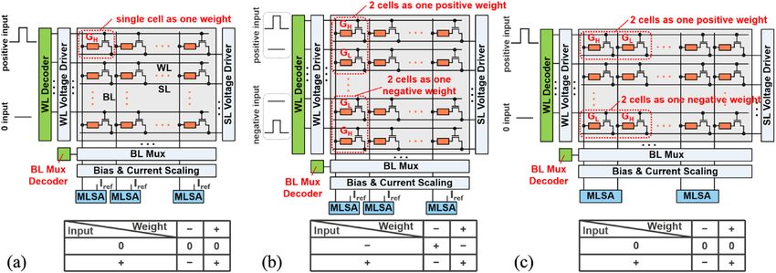
www.nature.com/scientificreports/
Figure 3. DtD conductance (G) variation of memory states fit the log-normal distribution in (a) STT-MRAM,
(b) FTJ23, (c) MLC PCM5, (d) MLC RRAM6. The standard deviations (σ) do not change significantly in the same
device except for the lowest G (00) state in MLC PCM and RRAM. The higher variation of the (00) state has less
impact on IMC accuracy. Thus, we adopted a constant σ in the log-normal distribution as the variation model.
Figure 4. Weight distribution of 3-bit linear quantization (S-MLC, GH/GL = 10, σ = 0.05). (a) N-IMC mapping.
Variation is higher at + w with high conductance in the linear scale. (b) WS-IMC mapping. Variation is
symmetric at + w and − w.
symmetric for ± w in WS-IMC (Fig. 4b). This is because the same conductance difference of two adjacent cells
is used to represent the value of the signed weights. Although C-IMC utilizes two cells in the same column to
represent one weight, only one cell between the two is accessed at a time because of the complementary inputs
applied to the transistor gate terminal of the 1T1R cell. Therefore, both the weights of C-IMC and N-IMC
schemes are based on the difference between the device conductance of one cell and the reference. So the weight
distribution of C-IMC is identical to that of N-IMC.
Quantization policy for accurate inference. All three schemes discussed in “DNN-to-IMC mapping”
section could achieve comparable accuracy after appropriately training the models when the device variation is
negligible. However, their immunity against device variation differs substantially. Figure 5 shows the inference
accuracy of VGG-9 DNNs for CIFAR-10 classification with different levels of variability. The weight placement
considering the log-normal conductance distribution and G-independent σ was evaluated using the Monte Carlo
simulation of at least 200 times. The distribution of these 200 data points was plotted in Fig. 5. As σ increases, the
inference accuracy degrades. N-IMC is the worst mainly due to the error accumulation from + w with broader
distributions of GL states as compared with − w, as apparent in Fig. 4a. C-IMC shows improvement on inference
accuracy compared with N-IMC because of the error cancellation effect originated from the complementary
input. Note that the generation of complementary inputs requires additional hardware cost. WS-IMC is the most
superior against variation among three because of the error cancellation from the symmetric and tighter ± w
distribution (Fig. 4b) that is constituted by two cells but not one, and it requires no complementary input. More
detailed comparison between these three schemes with different GH/GL could be found in Fig. S2 (Supporting
Information). For the rest of this paper, only the median values of inference accuracy in the Monte Carlo simula-
tion and the WS-IMC mapping scheme are discussed for simplicity.
Besides DNN-to-IMC mapping schemes, different design considerations at the algorithm and device levels
also affect the inference accuracy in the presence of device variation. In the following subsections, we will further
discuss the impact of choices of networks and datasets, quantization function, weight (conductance) precision,
and dynamic range on inference accuracy.
Scientific Reports | (2022) 12:112 | https://doi.org/10.1038/s41598-021-04159-x 4
Vol:.(1234567890)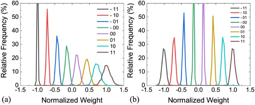
www.nature.com/scientificreports/
Figure 5. Influence of IMC mapping schemes. CIFAR-10 inference accuracy using VGG-9, 1-bit weight, 1-bit
activation, GH/GL = 100 are compared. The statistical effect of conductance variation was evaluated using the
Monte Carlo simulation of at least 200 times.
Figure 6. (a) CIFAR-10 inference accuracy comparison using linear and logarithmic quantization with
variations. 3-bit weight, GH/GL = 100, and WS-IMC mapping are used. The distribution of different quantized
weight levels using (b) linear and (c) logarithmic quantization.
Network choice. Variation immunity is known to be sensitive to the choice of DNN algorithms8. Both VGG-16
and ResNet-18 are compared by using a more complex Tiny ImageNet dataset, as shown in Fig. S3 (Supporting
Information). The compact ResNet-18 with 11.4 M parameters deteriorates the variation immunity compared
with the VGG-16 with 134.7 M parameters8. For example, for a device with 1-bit weight, GH/GL = 100, and
σ = 0.1, the accuracy for ResNet-18 and VGG-16 are 39.82% and 47.57%, respectively. Therefore, only the VGG-
DNNs with better immunity against variation are further evaluated below.
Lin‑Q vs. Log‑Q. Logarithmic quantization (Log-Q) is favored for multi-bit memory storage because a larger
memory sensing margin is possible by avoiding overlapping of tailed bits between levels. Previous studies also
attempted to use Log-Q for the weights of D NNs24. Our simulation shows that after appropriate training both
Log-Q and Lin-Q achieve comparable accuracy in the ideal quantization case without variation. However, Lin-Q
shows more robust immunity against variation than Log-Q, as shown in Fig. 6. This is explained by their differ-
ent weight distributions. In Log-Q, more weights are located at ± 11 states which have a wider weight distribu-
tion. Therefore, the larger sensing margin between levels in Log-Q does not necessarily guarantee better immu-
nity against variation. Only Lin-Q is further discussed in this study.
Scientific Reports | (2022) 12:112 | https://doi.org/10.1038/s41598-021-04159-x 5
Vol.:(0123456789)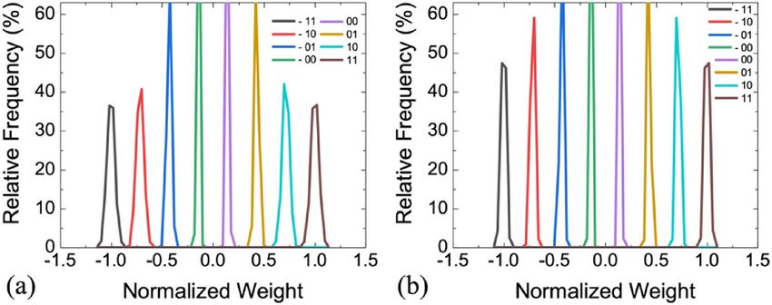
www.nature.com/scientificreports/
Figure 7. Impact of linear quantization policy considering weight precision and GH/GL. (a) CIFAR-10 inference
(VGG-9) accuracy using GH/GL = 2 and GH/GL = 100. (b) Tiny ImageNet inference (VGG-16) using GH/GL = 2
and GH/GL = 100. 1-bit activation is assumed. Higher weight precision improves the baseline accuracy but is
more susceptible to variation. Enlarging GH/GL improves immunity against variation.
Weight quantization precision and dynamic range. The immunity to variation is further investigated in the
models with different weight precision from one to three bits in Fig. 7. The focus on the lower weight precision
considers only inference but not training applications and also the reality of using the existing memory technol-
ogy for realizing MLC. Here we also take into account the influence of conductance dynamic range GH/GL. The
major conclusions are: (1) Although the high weight precision improves the baseline accuracy in the ideal case,
it is more susceptible to variation. The accuracy could be even worse than using low weight precision if the vari-
ation is substantial. For the first order, this effect could be explained as follows: For a higher weight precision, a
larger number of weight states are placed within a given dynamic range. The margin between each state becomes
less compared with the case with a lower weight precision. The same degree of variation (same σ) would distort
the pre-trained model more significantly and result in more severe accuracy degradation. (2) Enlarging the
dynamic range is beneficial to the variation immunity for a given σ. However, at the same normalized σ, i.e. σ/
ln(GH/GL), a smaller dynamic range with smaller device variation is favorable than a larger dynamic range with
larger device variation, as shown in Fig. 8. The result suggests that a low absolute value of σ is still critical for
the model accuracy. Higher priority should be given to suppressing variation rather than enlarging the dynamic
range. (3) A more complicated dataset (Tiny ImageNet vs. CIFAR-10) is more susceptible to variation since the
model itself also becomes more complicated, but it does not change the general trends aforementioned.
Variation‑aware accurate DNN. Two approaches are further evaluated to improve the immunity against vari-
ation. First, the D-MLC and A-MLC weights, as introduced in “Quantized weight” section, are more robust
against variation than the S-MLC weight. Figure 9 shows an example of the weight distribution of 3-bit lin-
ear quantization in the WS-IMC mapping scheme by using the D-MLC and A-MLC weight, respectively. The
D-MLC and A-MLC weights consist of three and seven binary (1-b) memory cells, respectively, with the identi-
cal GH/GL and σ as those in Fig. 4b for the S-MLC weight. Because more cells are used to represent a weight for
D-MLC and A-MLC, the “effective” σ for a given quantized weight precision is reduced due to the averaging
effect from the law of large numbers. Second, the inference accuracy degradation could be partially recovered by
fine-tuning the last fully-connect classifier layer in the network7. The last classifier layer is a full-precision layer
that could be easily implemented using the conventional digital circuits. After placing weights in all IMC lay-
ers, the weights in the digital classifier layer is retrained with all weights in the IMC layers fixed. The computing
Scientific Reports | (2022) 12:112 | https://doi.org/10.1038/s41598-021-04159-x 6
Vol:.(1234567890)
www.nature.com/scientificreports/
Figure 8. Normalized σ vs. accuracy and the impact of dynamic range and weight precision. σ is normalized to
ln(GH/GL) considering the log-normal distribution of variation in memory states.
Figure 9. Weight distribution of 3-bit linear quantization (GH/GL = 10, σ = 0.05 for 1-bit cell) using (a)
the WS-IMC + D-MLC mapping scheme and (b) the WS-IMC + A-MLC mapping scheme, showing tighter
distributions than S-MLC in Fig. 4b.
efforts for retraining only the classifier layer is relatively small. The retrain speed is fast because it requires only
a subset of data instead of a complete training epoch7.
Tables 2 and 3 summarize the maximum tolerable variation for CIFAR-10 and Tiny ImageNet, respectively, by
using different quantization policies, including quantization precision, dynamic range, and weight implementa-
tion scheme. The pre-defined target accuracy for CIFAR-10 using VGG-9 and Tiny ImageNet using VGG-16 are
88% and 48%, respectively. To achieve the proposed targets with relatively high accuracy, higher weight preci-
sion (2/3b vs. 1b) is beneficial because it increases the baseline accuracy, thus allowing more variation tolerance.
Enlarging GH/GL is also beneficial. Among the three weight implementation schemes, A-MLC shows the best
variation tolerance due to its smallest “effective” σ obtained from multiple devices. Furthermore, the fine-tuning
technique is extremely useful for boosting variation tolerance. So it should be applied whenever possible if
device-level solutions for reducing σ are not available.
Variation‑aware PPA co‑optimization. Some of the strategies for improving IMC variation immunity
accompany penalties in power and area. A larger GH/GL implies that the GH cell is forced to operate in a higher
current regime. Here we assume the minimum of GL is finite and limited by the leakage in given memory tech-
nology. Previous studies have shown that a high BL current creates substantial voltage drop on the parasitic line
resistance and results in inaccurate MAC results. Partitioning a large array with high BL currents to smaller ones
is necessary to guarantee the model accuracy23. The higher GH thus restricts the attainable maximum sub-array
size because of the excessively large accumulated current on BLs. The increased BL current with higher GH dete-
riorates energy efficiency while the smaller sub-arrays with higher GH deteriorates area efficiency due to higher
peripheral circuit overhead. D-MLC and A-MLC by using more memory cells also increase the area and energy
consumption of IMC. Therefore, the variation tolerance should be carefully traded off with efficient hardware
design. To fairly evaluate the PPA of IMC with different device specifications, we completed a reference design
based on the foundry 40-nm CMOS technology with a 256 × 256 1T1R RRAM array macro. The major circuit
blocks in the macro are similar to the illustration shown in Fig. 1. We assume a hypothetical memory with a
fixed low conductance state (GL = 0.5 μS) and GH/GL = 10, 1-bit input/activation, and the WS-IMC/S-MLC map-
Scientific Reports | (2022) 12:112 | https://doi.org/10.1038/s41598-021-04159-x 7
Vol.:(0123456789)
www.nature.com/scientificreports/

                                            Dynamic range   Weight precision   Weight implemented scheme   Tolerable STD w/o FT   Tolerable STD w/ FT
                                                            1-bit              S-MLC                       0.05                   0.07
                                                                               S-MLC                       0.08                   0.11
                                                            2-bit              D-MLC                       0.11                   0.15
                                            GH/GL = 2                          A-MLC                       0.14                   0.19
                                                                               S-MLC                       0.08                   0.11
                                                            3-bit              D-MLC                       0.12                   0.27
                                                                               A-MLC                       0.2                    0.28
                                                            1-bit              S-MLC                       0.1                    0.17
                                                                               S-MLC                       0.2                    0.29
                                                            2-bit              D-MLC                       0.24                   0.37
                                            GH/GL = 100                        A-MLC                       0.26                   0.46
                                                                               S-MLC                       0.22                   0.3
                                                            3-bit              D-MLC                       0.27                   0.66
                                                                               A-MLC                       0.33                   0.66

                                           Table 2.  Tolerable variation for CIFAR-10 (VGG-9 @ 88% acc.) with and without fine-tuning (FT).

                                            Dynamic range   Weight Precision   Weight implemented scheme   Tolerable STD w/o FT   Tolerable STD w/ FT
                                                            1-bit              S-MLC                       0.03                   0.08
                                                                               S-MLC                       0.05                   0.1
                                                            2-bit              D-MLC                       0.06                   0.12
                                            GH/GL = 2                          A-MLC                       0.08                   0.16
                                                                               S-MLC                       0.05                   0.1
                                                            3-bit              D-MLC                       0.08                   0.16
                                                                               A-MLC                       0.13                   0.27
                                                            1-bit              S-MLC                       0.08                   0.27
                                                                               S-MLC                       0.13                   0.24
                                                            2-bit              D-MLC                       0.14                   0.27
                                            GH/GL = 100                        A-MLC                       0.18                   0.39
                                                                               S-MLC                       0.13                   0.25
                                                            3-bit              D-MLC                       0.17                   0.37
                                                                               A-MLC                       0.22                   0.61

                                           Table 3.  Tolerable variation for Tiny ImageNet (VGG-16 @ 48% acc.) with and without fine-tuning (FT).

                                           Figure 10.  (a) Area and (b) power breakdown of a 40 nm 256 × 256 1T1R IMC macro.

          Scientific Reports |   (2022) 12:112 |                https://doi.org/10.1038/s41598-021-04159-x                                              8

Vol:.(1234567890)
www.nature.com/scientificreports/
Figure 11. Area and energy estimation of feasible IMC designs that guarantees CIFAR-10 inference (VGG-
9) with at least 88% accuracy (see Table 2). Designs considering different standard deviation of conductance
distribution, GH/GL ratio, and S-MLC/D-MLC/A-MLC scheme are compared, and the lowest possible weight
precision is used to simplify the hardware implementation. 1-bit activation is assumed. Dark and light colors
indicate the estimation w/o and w/ considering fine-tuning. The fine-tuning results are shown only when fine-
tuning helps to reduce the weight precision required. The lowest weight precision required is also indicated.
ping. The IMC sub-array size is limited by the maximum allowed BL current of 300 μA through current-mode
sensing. Fig. 10 shows a simulated power and area breakdown of the IMC macro, which includes bias clamping
and current scaling circuits, current-mode SAs, analog adders to accumulate the partial sums from different
sub-arrays, and driver circuits for WL/BL/SL. Other IMC designs using different GH/GL ratios (assuming G L is
fixed), D-MLC/A-MLC weights, multi-cycle inputs, and multibit ADCs are then extrapolated using the refer-
ence design.
The area and energy of feasible designs for VGG-9 that satisfy the pre-defined accuracy target (e.g. Table 2)
are compared in Fig. 11. The trends for VGG-16 are similar and not shown here. The lowest weight precision is
used whenever possible to relax device requirements and system overhead. The energy is estimated by the total
energy consumption of 10,000 CIFAR-10 inferences. We summarize the strategies on the PPA co-optimization as
follows: (1) For a low-variation device (σ = 0.05), a binary cell with low GH/GL allows the highest area and energy
efficiency. (2) For a moderate-variation device (σ = 0.15), S-MLC with moderate GH/GL (< 10) achieves better
efficiency. (3) For a high-variation device (σ = 0.25), using S-MLC becomes challenging unless the fine-tuning
is considered. Using D-MLC/A-MLC with moderate GH/GL is practical alternatives to maintain accuracy at a
reasonable cost of energy and area. Other variation-aware strategies that could affect the PPA of IMC include
using a higher (3-bit) input/activation precision and more channels (2 times more) in a wider VGG network.
The complete area and energy estimations of these variation-aware strategies are shown in Fig. S4 (Supporting
Information). Only those most efficient schemes using the lowest possible bit precision for satisfying the target
accuracy are plotted in Fig. 12 for each dynamic range. Our evaluations show that the substantial penalties on
area and energy restrict these strategies only competitive in specific conditions, especially when σ is large.
Conclusion
In this paper, we provided an end-to-end discussion for the impact of intrinsic device variation on the system
PPA co-optimization. We considered critical device-level constrains, such as limited quantization precision and
memory dynamic range, circuit-level constraints, such as limited current summing capability and peripheral
circuit overhead, architecture-/algorithm-level options, such as DNN-to-IMC mapping schemes, types of DNN
algorithms, and using multiple cells for representing a higher-precision weight.
The WS-IMC mapping scheme, DNN-like algorithm, and linear quantization shows more robust immunity
against variation. Although higher weight precision of S-MLC improves the baseline accuracy, it is also more
susceptible to variation when the variation is high and the dynamic range is low. Multiple cells per weight and
Scientific Reports | (2022) 12:112 | https://doi.org/10.1038/s41598-021-04159-x 9
Vol.:(0123456789)
www.nature.com/scientificreports/
Figure 12. Area and energy estimation of IMC designs using the same criteria as Fig. 11 but with either wider
channel or 3-bit activation. The improvements only exist in specific conditions with high σ.
fine-tuning are two effective approaches to suppress inference accuracy loss if device-level solutions for reducing
variation are not available. As for the PPA co-optimization, we found that memory devices with a large number
of analog states spanning in a wide dynamic range do not necessarily lead to better IMC design. Low-bit MLC
or even binary memory technology with G RAM25 and F
H/GL < 10 and low variability, e.g. binary M TJ23 with low
conductance, deserves more attention.
Methods
Network structure. VGG-9 network for CIFAR-10 classification consists of 6 convolutional layers and 3
fully connected classifier layers. Image is processed through the stack of convolutional layers and 3 × 3 filters with
a stride of 1. Max-pooling is performed over a 2 × 2 window and follow every 2 convolutional layers. Batch nor-
malization and hard tanh as activation function are applied to the output of each convolutional layer. The width
of convolutional layers starts from 128 in the first layer and increasing by a factor of 2 after each max-pooling
layer. For the positive only IN in N-IMC and WS-IMC, the output of hard tanh activation function is scaled and
normalized between 0 and 1.
VGG-16 network for Tiny ImageNet classification consist of 13 convolutional layers and 3 fully connect
layer. Max-pooling is performed over a 2 × 2 window and follow every 2 or 3 convolutional layers. The width of
convolutional layers starts from 64 in the first layer and increasing by a factor of 2 after each max-pooling layer.
Quantized neural network training. We use quantize weights and activation to perform VMM calcula-
tion at run-time and compute parameter gradients at train-time, while the real-valued gradients of the weight
are accumulated in real-value variable. Real-value weights are required for optimizer to work at all. The quan-
tized weights and activations are transformed from the real-value variable by using the following deterministic
linear quantization function:
x
r
xQ = LinQ(xr , bitwidth) = Clip , min, max ,
bitwidth
and logarithmic quantization function
Scientific Reports | (2022) 12:112 | https://doi.org/10.1038/s41598-021-04159-x 10
Vol:.(1234567890)www.nature.com/scientificreports/
xQ = LogQ(xr , bitwidth) = Clip sign(xr ) × 2round(log2|xr |) , min, max ,
where xr is the original real-value variable, xQ is the value after quantization, bitwidth is quantization bit preci-
sion, and min and max are the minimum and maximum scale range, r espectively24.
The real-valued weight gets updated iteratively by using adaptive moment estimation (ADAM) optimization
algorithm using the learning rate decayed by half every 20 or 40 epochs. Both CIFAR-10 and Tiny ImageNet
datasets are trained over 200 epochs with a batch size of 256. All the results are obtained with PyTorch, a popular
machine learning framework, and trained on an NVIDIA Tesla P100 GPU.
Received: 12 July 2021; Accepted: 15 December 2021
References
1. Ielmini, D. & Wong, H.-S.P. In-memory computing with resistive switching devices. Nat. Electron. 1, 333–343 (2018).
2. Chang, C.-C. et al. Challenges and opportunities toward online training acceleration using RRAM-based hardware neural network.
In IEEE Int. Electron Devices Meeting (IEDM), 278–281 (2017).
3. Hubara, I., Courbarizux, M., Soudry, D., El-Yaniv, R. & Bengio, Y. Quantized neural networks: Training neural networks with low
precision weights and activations. J. Mach. Learn. Res. 18, 6869–6898 (2018).
4. Hashemi, S., Anthony, N., Tann, H., Bahar, R. I. & Reda, S. Understanding the impact of precision quantization on the accuracy
and energy of neural networks. In Design Automation Test Europe (DATE), 1474–1483 (2017).
5. Nirschl, T. et al. Write strategies for 2 and 4-bit multi-level phase-change memory. In IEEE International Electron Devices Meeting
(IEDM), 461–464 (2007).
6. Chang, M.-F. et al. A high-speed 7.2-ns read-write random access 4-Mb embedded resistive RAM (ReRAM) macro using process-
variation-tolerant current-mode read schemes. IEEE J. Solid-State Circuits 48, 878–891 (2013).
7. Chang, C.-C. et al. NV-BNN: An accurate deep convolutional neural network based on binary STT-MRAM for adaptive AI edge.
In ACM/IEEE Design Automation Conference (DAC) (2019).
8. Yang, T-J. & Sze, V. Design considerations for efficient deep neural networks on processing-in-memory accelerators. In IEEE
International Electron Devices Meeting (IEDM), 514–517 (2019).
9. Yan, B., Liu, M., Chen, Y., Chakrabarty, K. & Li, H. On designing efficient and reliable nonvolatile memory-based computing-in-
memory accelerators. In IEEE International Electron Devices Meeting (IEDM), 322–325 (2019).
10. Welser, J., Pitera, J. W. & Goldberg, C. Future computing hardware for AI. In IEEE International Electron Devices Meeting (IEDM),
21–24 (2018).
11. Szeliski, R. Computer Vision: Algorithms and Applications (Springer, 2010).
12. Hu, M. et al. Dot-product engine for neuromorphic computing: Programming 1T1M crossbar to accelerate matrix-vector multi-
plication. In ACM/IEEE Design Automation Conference (DAC) (2016).
13. Shafiee, A. et al. ISAAC: A convolutional neural network accelerator with in-situ analog arithmetic in crossbars. In ACM/IEEE
43rd International Symposium on Computer Architecture (ISCA), 14–26 (2016).
14. Chen, P-Y. et al. Mitigating effects of non-ideal synaptic device characteristics for on-chip learning. In ACM/IEEE International
Conference on Computer-Aided Design (ICCAD), 194–199 (2015).
15. Sun, X. et al. XNOR-RRAM: A scalable and parallel resistive synaptic architecture for binary neural networks. In Design Automa‑
tion Test Europe (DATE), 1423–1428 (2018).
16. Yin, S., Jiang, Z., Seo, J.-S. & Seok, M. XNOR-SRAM: In-memory computing SRAM macro for binary/ternary deep neural networks.
IEEE J. Solid-State Circuits (JSSC) 55, 1–11 (2020).
17. Burr, G. W. et al. Large-scale neural networks implemented with non-volatile memory as the synaptic weight element: comparative
performance analysis (accuracy, speed, and power). In IEEE International Electron Devices Meeting (IEDM), 76–79 (2015).
18. Chi, P. et al. PRIME: A novel processing-in-memory architecture for neural network computation in ReRAM-based main memory.
In ACM/IEEE 43rd International Symposium on Computer Architecture (ISCA), 27–39 (2016).
19. Chen, W.-H. et al. A 65nm 1Mb nonvolatile computing-in-memory ReRAM macro with sub-16ns multiply-and-accumulate for
binary DNN AI edge processors. In IEEE International Solid-State Conference (ISSCC), 494–496 (2018).
20. Xue, C.-X. et al. A 1Mb multibit ReRAM computing-in-memory macro with 14.6ns parallel MAC computing time for CNN based
AI edge processors. In IEEE International Solid-State Conference (ISSCC), 388–390 (2019).
21. Wu, W. et al. Improving analog switching in HfOx-based resistive memory with a thermal enhanced layer. IEEE Electron Device
Lett. 38, 1019–1022 (2017).
22. Ambrogio, S. et al. Reducing the impact of phase change memory conductance drift on the inference of large-scale hardware neural
networks. In IEEE International Electron Devices Meeting (IEDM), 110–113 (2019).
23. Wu, T-Y. et al. Sub-nA low-current HZO ferroelectric tunnel junction for high-performance and accurate deep learning accelera-
tion. In IEEE International Electron Devices Meeting (IEDM), 118–121 (2019).
24. Miyashita, D., Lee, E. H. & Murmann, B. Convolutional neural networks using logarithmic data representation. http://arXiv.org/
1603.01025 (2016).
25. Doevenspeck, J. et al. SOT-MRAM based analog in-memory computing for DNN inference. In IEEE Symposium on VLSI Technol‑
ogy (VLSIT), JFS4.1 (2020).
Acknowledgements
This work was supported in part by the Ministry of Science and Technology, Taiwan, under Grant
109-2221-E-009-020-MY3, 110-2634-F-009-017, 110-2622-8-009-018-SB and 109-2634-F-009-022, 109-2639-
E-009-001 and TSMC.
Author contributions
C.C. and T.H. carried out the experiments and analyzed the data. C.C. and T.H. wrote the manuscript. All authors
discussed the results and contributed to the final manuscript.
Competing interests
The authors declare no competing interests.
Scientific Reports | (2022) 12:112 | https://doi.org/10.1038/s41598-021-04159-x 11
Vol.:(0123456789)www.nature.com/scientificreports/
Additional information
Supplementary Information The online version contains supplementary material available at https://doi.org/
10.1038/s41598-021-04159-x.
Correspondence and requests for materials should be addressed to T.-H.H.
Reprints and permissions information is available at www.nature.com/reprints.
Publisher’s note Springer Nature remains neutral with regard to jurisdictional claims in published maps and
institutional affiliations.
Open Access This article is licensed under a Creative Commons Attribution 4.0 International
License, which permits use, sharing, adaptation, distribution and reproduction in any medium or
format, as long as you give appropriate credit to the original author(s) and the source, provide a link to the
Creative Commons licence, and indicate if changes were made. The images or other third party material in this
article are included in the article’s Creative Commons licence, unless indicated otherwise in a credit line to the
material. If material is not included in the article’s Creative Commons licence and your intended use is not
permitted by statutory regulation or exceeds the permitted use, you will need to obtain permission directly from
the copyright holder. To view a copy of this licence, visit http://creativecommons.org/licenses/by/4.0/.
© The Author(s) 2022
Scientific Reports | (2022) 12:112 | https://doi.org/10.1038/s41598-021-04159-x 12
Vol:.(1234567890)You can also read