DSVP: Dual-Stage Viewpoint Planner for Rapid Exploration by Dynamic Expansion
←
→
Page content transcription
If your browser does not render page correctly, please read the page content below
DSVP: Dual-Stage Viewpoint Planner for Rapid Exploration by
Dynamic Expansion
Hongbiao Zhu1,2 , Chao Cao1 , Yukun Xia1 , Sebastian Scherer1 , Ji Zhang1 , and Weidong Wang2
Abstract— We present a method for efficiently exploring
highly convoluted environments. The method incorporates two
planning stages - an exploration stage for extending the
boundary of the map, and a relocation stage for explicitly
transiting the robot to different sub-areas in the environment.
The exploration stage develops a local Rapidly-exploring Ran-
dom Tree (RRT) in the free space of the environment, and
the relocation stage maintains a global graph through the
mapped environment, both are dynamically expanded over
replanning steps. The method is compared to existing state-
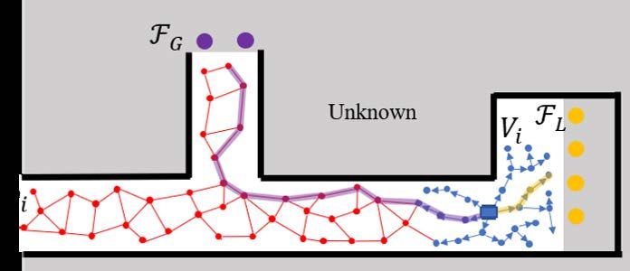
Fig. 1: Illustration of our method. The grey area stands for the
of-the-art methods in various challenging simulation and real
unknown space. The black solid lines are the obstacles , i.e. the
environments. Experiment comparisons show that our method
occupied space. The blue solid rectangle is the robot. The purple
is twice as efficient in exploring spaces using less processing
dots in the unknown space are the global frontiers FG , while
than the existing methods. Further, we release a benchmark
the yellow dots are the local frontiers FL . The blue dots, local
environment to evaluate exploration algorithms as well as
viewpoints Vi , and blue arrows form the local tree. The red dots
facilitate development of autonomous navigation systems. The
and red lines make up the global graph. Those red dots are the
benchmark environment and our method are open-sourced.
global vertices vi , which are viewpoints as well. The yellow and
I. I NTRODUCTION purple semi-transparent lines are exploration and relocation paths.
Autonomous exploration tackles the problem of deploying the coverage of all underlying viewpoints on the branch. Our
robots in environments unknown a priori for information method extends the framework in mainly two aspects.
gathering. This problem is essential for fulfilling tasks such • Dynamic Expansion: Both stages dynamically expand
as search, rescue, and survey. Yet, it remains challenging due the RRT and graph, respectively, over replanning steps.
to the complex structural setting and geometric layout in the Nodes on the RRT that are occluded or out of the
environment. Very often, the environment to be explored is planning horizon are trimmed off. Then, new nodes are
convoluted, consisting of branches connected at intersections. sampled in the free space. This way, useful viewpoints
The robot needs to transit between sub-areas in order to are kept, while newly sampled viewpoints further en-
efficiently explore the environment. force the solution. Further, much computation is saved
The paper puts forward a method capable of efficiently not re-building the entire RRT at each replanning step.
exploring environments at a high-degree of convolution. The • Hybrid Frontiers: The method uses a combination of
method incorporates two planning stages - an exploration frontiers extracted in the sensor range associated with
stage in charge of extending the boundary of the map, and a the RRT nodes as well as frontiers extracted in the sur-
relocation stage for explicitly transiting the robot to different roundings of the robot. Due to the randomness of RRT,
sub-areas in the environment (see Fig. 1). The exploration using any single type of frontiers or none often results
stage uses a local Rapidly-exploring Random Tree (RRT) [1] in certain areas in the environment being overlooked.
to span the space in the surroundings of the robot, searching Our method uses both types of frontiers to guide the
for the branch on the RRT leading to the highest collective expansion of the RRT, ensuring complete coverage.
reward for the robot to execute. The relocation stage involves In addition to the above theoretical contributions, we
a global graph built along the course of the exploration, release a benchmark environment1 containing representative
keeping a record of fully and partially covered areas. During simulation environments, fundamental navigation modules,
deployment, the robot transitions back-and-forth between the e.g. collision avoidance, terrain traversability analysis, way-
two stages to explore all areas in the environment. point following, and visualization tools for benchmarking
Our method draws inspiration from a well-known explo- exploration algorithms. The environment is also meant to
ration algorithm framework [2]. Such a framework expands facilitate development of autonomous navigation systems.
a RRT in the free space and considers nodes on the RRT as Our exploration method is evaluated in the benchmark
viewpoints. Sensor coverage is estimated from each view- environment and physical experiment where the robot ex-
point. Computing the reward of each branch accounts for plores an area containing multiple buildings on the university
1 H. Zhu, C. Cao, Y. Xia, S. Scherer, and J. Zhang are with the Robotics campus. In all evaluated environments, our method signifi-
Institute at Carnegie Mellon University, Pittsburgh PA. cantly outperforms the state-of-the-art methods in terms of
2 H. Zhu and W. Wang are with the Robotics Institute at Harbin Institute
of Technology, Harbin China. 1 Benchmark environment: https://www.cmu-exploration.com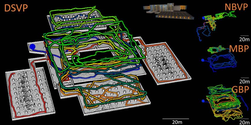
exploration efficiency. Our method is open-sourced2 and our      hybrid frontiers. We compare our method with NBVP [2],
experiment results are available in a public video3 .            MBP [12], and GPB [13] in various simulation and real-
                                                                 world environments. We conclude that our method produces
                   II. R ELEATED W ORK                           more complete coverage and the exploration efficiency is
   In recent years, numerous techniques have been devel-         more than twice of the state-of-the-art while the processing
oped to solve the autonomous exploration problem, such as        load is less.
frontiers-based algorithm [3]–[9], next-best-view algorithms
                                                                                      III. M ETHODOLOGY
[2], [10]–[13] and algorithms based on machine learning
                                                                                  3
[14]–[17]. The previous two types of algorithm are com-             Define S ⊂ R as the space to be explored. Let Sf ree ⊂ S
monly used in most exploration methods while machine             be the known free space, Socc ⊂ S be the known occupied
learning based approaches have emerged recently.                 space and Sunk ⊂ S be the current unknown space. As
   Frontier-based approach is among the most effective ways      shown in Fig. 1, at the exploration stage of our method,
in exploration. In frontier-based algorithms, one important      a dynamically-expanded RRT is used to create the local
issue to solve is the sequence to visit frontiers. Method in     random tree, the nodes of which are viewpoints. The best
[3] selects the closest frontier as the goal, often causing      branch is then obtained and taken as the trajectory by
repeated visits during the exploration. Approach [4] makes       computing the reward of each branch in the tree. In this
improvements by using a repetitive rechecking method and         stage, frontiers that are within the field of view of the robot
segmenting the environment into small pieces. Since the          as well as the RRT nodes are extracted as local frontiers. At
segmentation is adapted to structured indoor environments,       the relocation stage, global frontiers, which are made up of
the method only works well indoors. Traveling Salesman           the local frontiers that are not cleared until the latest update,
Problem (TSP) is later employed in [5], [18] to get the          assist the planner to choose the best one from all remaining
sequence of visiting all frontiers. However, as more frontiers   viewpoints in the global graph.
are generated along the exploration, the TSP becomes larger
and heavier to solve. In [19], instead of taking frontiers as    A. Exploration Stage
goals, viewpoints that can see all frontiers are generated and      Our method uses dynamically-expanded RRT at the explo-
a generalized TSP is used to obtain the best sequence to visit   ration stage to generate viewpoints around the robot in each
the viewpoints.                                                  iteration. Fig. 2 shows the process of dynamic expansion.
   In contrast, next-best-view approaches do not use frontiers   As shown in Fig. 2a, define H ⊂ R3 , the green square, as
as the direct guidance or goals, but use randomly sam-           the planning horizon and set the current position PR , point
pled viewpoints in the free space. Next Best View Planner        A, as the root of the tree. Then, a RRT is constructed at
(NBVP) [2] is considered the state-of-art in this category.      the first iteration, before which there is no previous RRT.
It generates viewpoints with RRTs and then computes the          All nodes on the tree are viewpoints, defined as V . we
volumetric gain of each viewpoint. Yet, its major limitation     use octomap [21] as the underlying occupancy map, with
is that it only focuses on the process of extending the map      which the collision check of viewpoints and edges between
boundary. The method is limited in transiting to different       viewpoints are performed to ensure they are in the free space.
areas in the environment for further exploration, after one      When the robot moves to point B in Fig. 2b after an iteration,
area is fully explored. A method named Graph-Based ex-           the previous tree is reconstructed in two steps. First, the tree
ploration Planner (GBP) [13] develops a global Rapidly-          is pruned by deleting all nodes that are occluded or out of the
exploring Random Graph (RRG) [20] to re-position the             current planning horizon H, such as the light blue nodes in
robot to unexplored areas. Another method named Motion-          Fig. 2b. Next, we update the tree structure so that PR , point
primitive-Based exploration Planner (MBP) [12] develops the      B, becomes the root of the new tree. New viewpoints, orange
local RRT using motion primitives. The resulting paths are       nodes in Fig. 2b, are randomly sampled and added to the
smoother and span in constrained directions. However, all the    new tree. With the dynamic expansion, only a small fraction
three methods expand a new RRT or RRG at each replanning         of nodes are re-generated in each iteration, which results in
step in the exploration mode. A large number of useful           less computation compared to completely constructing a new
nodes are removed and re-sampled, wasting computation.           tree. In addition, we prune nodes that are in collision due to
Further, since RRT and RRG expand randomly in the free           dynamic obstacles and thin structures previously overlooked
space, areas that are not spanned by the RRT or RRG are          by the sensor.
ignored. Consequently, the methods are prone to overlook            We use local frontiers FL to bias the tree construction
areas, especially for areas with small openings, and produce     during the exploration stage so that the tree expands towards
an incomplete coverage.                                          unknown areas along the previous direction of exploration.
   Our method extends the state-of-the-art methods by dy-        Local frontiers in this paper must meet the following condi-
namically maintaining and expanding the RRT during the           tions in Eq. (1)-(3).
exploration and guiding the expansion of the RRT with
                                                                                             FL ∈ B                           (1)
  2 DSVP  code: https://github.com/HongbiaoZ/dsv_planner
  3 Representative result: https://youtu.be/1yLLIZIIsDk                         ∃V s.t. FL is in F OV (V ) or                 (2)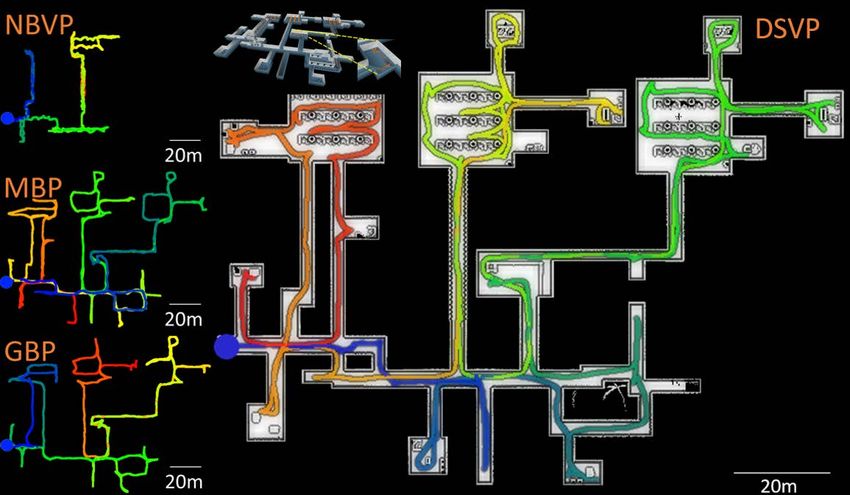
Algorithm 1: Exploration
                      FL is in F OV (PR )                         (3)     1   Set Slb , root position Prob and Flocal
                                                                          2   Update FLS
   In Eq.(1), B represents a boundary within which the local              3   V ← DynamicRRT()
frontiers are extracted. This region is slightly bigger than              4   BestGain ← 0
the planning horizon. Condition (2) and (3) require the                   5   for i from 1 to N do
frontier to be in the field of view (FOV) of at least one                 6       Compute Gain(Bi )
viewpoint or in the FOV of the robot. Note that line-of-                  7       if Gain(Bi ) > BestGain then
sight check is performed to ensure that the frontier can be               8            BestGain ← Gain(Bi )
observed by the viewpoint or the robot without occlusion.                 9            BestBranch ← Bi
In addition, terrrain traversability between the viewpoint or            10       end
the robot and frontiers are also taken into consideration to             11   end
make sure those frontiers are reachable. Under these two                 12   Previous Tree ← Current Tree
conditions, the hybrid frontiers that are around the viewpoints
and around the robots can be extracted. Note that when
extracting frontiers, the sensor range of the viewpoints is
set to smaller than that of the robot. This is because that              viewpoints close to the current exploration direction. With
viewpoints are expanded closer to frontiers, where a shorter             the guidance of local frontiers, the viewpoints distributed
range is sufficient for observing the fronteirs and can reduce           more densely near unknown areas in H. This can help make
overall computation. Condition (2) and (3) also serve as                 the sampling process more effective.
the noise-filtering process, where in complex environments                  Define V = {V1 , V2 , ..., Vn } as the set of viewpoints, where
occulusion and sensor noise can result in noisy frontiers that           the subscript indicates the order in which the corresponding
are not worth exploring. Given that frontiers are only used              viewpoint is generated. Eqs. (4) and 5 show the utility
as guidance, they can be grouped into sparse clusters.                   function used to compute the gain of each branch in the
   Among all FL , we select FLS to be the closest ones to                tree. It is similar to the method used in [13].
the current exploration direction. The selected frontiers bias
                                                                                                 X
                                                                                 Gain(Bi ) =            Gain(Vij ) · e−DT W (Bi )·λ1    (4)
the tree expansion as shown in Fig. 2b, where FLS1 , FLS2 ,
                                                                                                Vij ∈Bi
and FLS3 are the frontiers selected. The biased sampling
scheme is described as follows. We first uniformly sample                           Gain(V ) = V oxelGain(V ) · e−dist(V )·λ2          (5)
a number between 0 and 1. If the number is larger than
θ, a threshold for regulating the sampling area, then we                    where Bi represents the branch from root viewpoint
randomly sample points in the selected frontiers’ sensor                 V0 to Vi and Vij represents the jth viewpoint on Bi .
range. Otherwise, we sample points in other regions. The                 V oxelGain(V ) is the number of unknown voxels in the
probability of sampling points falling around the selected               FOV of viewpoint V . dist(V ) denotes the distance of the
frontiers is much higher than in other regions. Thus, the                tree branch from V0 to V , and λ1 is a parameter that
tree tends to expand towards the frontier, resulting in more             penalizes traveling distance. Function DT W (Bi ) is based
                                                                         on Dynamic Time Warping method [22] that computes the
                                                                         similarity between branch Bi and the branch selected in the
                                                                         last iteration, which also reflects the exploring direction. The
                                                                         more similar these two branches are, the lower the value of
                                                                         DT W (Bi ). λ2 is a parameter that penalizes the difference
                                                                         between Bi and the last trajectory. The branch with the
                                                                         greatest gain will be picked as the next trajectory.
                                                                            Algorithm 1 and 2 illustrate the process of the exploration
                                                                         stage. The local frontiers are updated at a constant frequency.
                                                                         FLS are selected from all local frontiers at the beginning
                                                                         of each iteration. Then, with the guidance of FLS , new
                (a)                               (b)                    viewpoints are sampled after pruning and reconstruction of
Fig. 2: Exploration stage. (a) shows the tree and local frontiers        the previous tree. Eventually, Eq. (4) is used to compute the
obtained in the previous iteration. Grey area is unknown space and       gain of each branch and determine the final trajectory.
black area is occupied space. Yellow solid circles are local frontiers
FL . The green square denotes the planning horizon H. (b) is the         B. Relocation Stage
new tree generated in the current iteration. The light blue dots are
pruned viewpoints that are out of the current planning horizon.
                                                                            When there is no local frontiers within the planning
Blue dots stand for useful viewpoints from the old tree and orange       horizon, the planner switches from the exploration stage to
dots are new sampled viewpoints. FLS1 , FLS2 and FLS3 are three          the relocation stage. The relocation stage involves the global
selected local frontiers used to guide the extension of local tree.      graph and global frontiers. The main utility of the global
Yellow hollow circles are the sensor ranges of the selected frontiers.   graph G is to record all the valuable viewpoints sampled at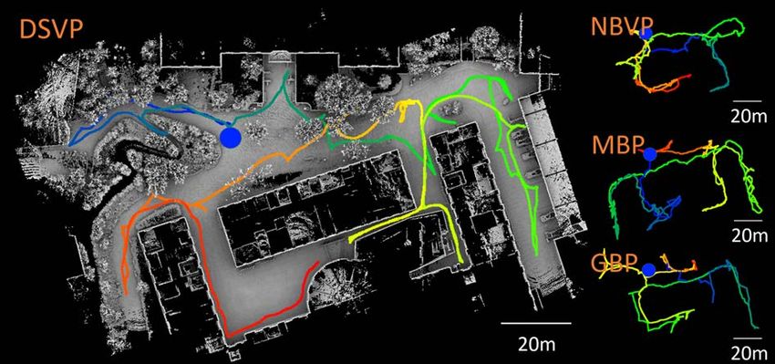
Algorithm 2: Dynamic Expansion                                      Algorithm 3: Relocation
1    Set Slb , root position Prob and FS                             1   Update Fglobal and G
2    Prune(Previous Tree)                                            2   F lag ← F alse and Dist ← 0
3    Rebuild(Previous Tree)                                          3   for i from N to 1 do
4    while Nnew < N do                                               4       for j from M to 1 do
 5       Sample u ∼ U [0, 1]                                         5           if Fi in FOV(vi ) then
 6       if u  γ
                                                                    25   end
where DE is the euclidean distance and DG is the closest
distance along the graph. δ and γ are two parameters to
restrict the euclidean distance and the ratio between the two
distances. Eq. (6) ensures that the graph is not too dense          can observe FGS , such as point A, which corresponds to
while providing short paths between vertices. Further, to           lines 16 to 23. After this process, the final target viewpoint
ensure that all edges in the graph are collision-free, we trim      vS is obtained. The robot then moves to vS along the graph
off edges that are in collision due to dynamic or previously        and enters exploration mode again. If no vertex is found in
overlooked obstacles. The graph is then adjusted after the          the first step, the exploration is completed, line 24. With
pruning to ensure connectivity. Note that vertices in the graph     global frontiers, this method guarantees all traversable areas
only includes position information, without considering the         are covered. In addition, there is no need to compute and
V oxelGain.                                                         update V oxelGain of each viewpoint in the global graph,
   Global frontiers FG are composed of local frontiers that         which saves much computation.
are left out previously. Note that they can be observed by                         IV. B ENCHMARK E NVIRONMENT
at least one viewpoint in the global graph. Every time the
                                                                      The environment serves as a platform for benchmarking
local frontiers are updated, they are added to FG . Meanwhile,
                                                                    exploration algorithms. It is also meant for leveraging sys-
all frontiers in FG are rechecked and removed if they are
cleared.
   The detailed process of the relocation stage is presented in
Algorithm 3. Define Fi as the ith frontier in FG , FGS as the
selected global frontier to be observed and vS as the vertex
that is selected as the goal. Taking Fig. 3 as an example. First,
the planner searches for a vertex that is able to observe any
global frontier in G determined by ray tracing. For a vertex
vi in G, the larger the value of i is, the later it appears and
the closer it is to the robot position. The same rule also
applies to the global frontiers. Thus, furthest global frontiers    Fig. 3: Relocation stage. The purple dots are global frontiers and the
                                                                    purple dot with blue edge is the selected global frontier FGS .The
are selected first, making the final selection close to the         red dots and red lines have the same definitions as Fig. 1. The green
current position. As in Fig. 3, point B is the vertex that can      viewpoint B is the first one that could observe FGS if searching
observe the selected frontier FGS . This process corresponds        from the end of the global graph. The green viewpoint A is the best
to lines 4 to 14 in Algorithm 3. Then the method searches           one to observe FGS .The yellow circles denote the sensor ranges of
the graph from the end again to find the closest vertex that        viewpoint A and B.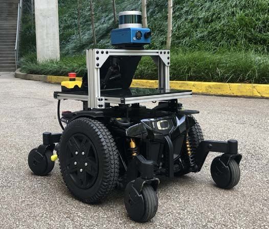
(a)                                    (b)
Fig. 4: (a) Collision avoidance. The yellow dots indicate collision-                        Fig. 5: System integration diagram
free paths. (b) Terrain map (40m x 40m). The green points are
traversable and the red points are non-traversable.                           traversable and the red points are non-traversable.
                                                                                 The visualization tools display the overall map and ex-
tem development and robot deployment for ground-based                         plored areas during the course of the exploration. Exploration
autonomous navigation. The environment contains a variety                     metrics such as explored volume, traveling distance, and
of simulation environments, fundamental navigation modules                    algorithm runtime are plotted and logged to inspect the
such as collision avoidance, terrain traversability analysis,                 performance. The environment is constructed with facili-
waypoint following, and a set of visualization tools. Table I                 tating development of autonomous navigation systems in
lists the characteristics of the simulation environments.                     mind. When integrated on a real robot, it takes the role as
  •   Campus (340m × 340m): A large-scale environment                         the middle layer in the autonomous navigation systems, as
      as part of the Carnegie Mellon University campus,                       illustrated in Fig. 5. Further, the environment supports using
      containing undulating terrains and convoluted layout.                   a joystick controller to interfere with the navigation, easing
  •   Indoor (130m × 100m): Consists of long and narrow                       the process of system debugging. Detailed information is
      corridors connected with lobby areas. Obstacles such as                 available on the project website (link provided on first page).
      tables and columns are present.                                                              V. E XPERIMENTS
  •   Garage (140m × 130m, 5 floors): An environment with
      multiple floors and sloped terrains to test autonomous                  A. Evaluation in Benchmark Environment
      navigation in a 3D environment.                                            We conduct simulation experiments with the benchmark
  •   Tunnel (330m × 250m): A large-scale environment                         environment in three environments, i.e. indoor, campus and
      containing tunnels that form a network, provided by                     garage. The vehicle navigates at 2 m/s. Our method sets the
      Tung Dang at University of Nevada, Reno.                                exploration planning horizon H to a 30m×30m area and the
  •   Forest (150m × 150m): Containing mostly trees and a                     frontier boundary B to a 40m×40m area. The resolution of
      couple of houses in a cluttered setting.                                the octomap is set to 0.35m. We compare with three state-of-
   The collision avoidance module [23] makes sure the                         art methods in the experiments, all using open-source code
vehicle navigates safely. It computes collision-free paths in                 adapted to the evaluation environments.
the vicinity of the vehicle and guides the vehicle to navigate                   • NBVP [2]: A method using RRT to span the space. It

between obstacles. The collision avoidance module utilizes                          finds the most informative branch in the RRT as the
pre-generated motion primitives. When the vehicle navigates,                        path to the next viewpoint.
it in real-time determines the motion primitives occluded                        • GBP [13]: An extension of NBVP where the method

by obstacles. The resulting collision-free paths, as shown in                       builds a global RRG through the traversable space and
Fig. 4a, are for vehicle navigation. The collision avoidance                        searches the RRG for routes to relocate the vehicle.
module takes as input the terrain maps from the terrain                          • MBP [12]: An extension of GBP where the method

analysis module to determine terrain traversability.                                builds the local RRT using motion primitives. The
   The terrain analysis module analyzes the local smoothness                        resulting paths are smoother and span in constrained
of the terrain and associates a cost to each point on the                           directions.
terrain map. This uses a voxel representation and checks the                  Each method is run 10 times. A run is ended if the explo-
distribution of the points in adjacent voxels. Advanced func-                 ration algorithm reports completion, the vehicle almost stops
tionalities such as handling negative obstacles are optional.                 moving (less than 10m of movement within 300s), or a time
Fig. 4b gives an example terrain map covering a 40m x 40m                     limit is reached. Here, the time limit is set to twice of the
area with the vehicle in the center. The green points are                     longest run of our method. Among the evaluated methods,
                                                                              only our method reports completion. In the following results,
        TABLE I: Simulation environment characteristics                       the trajectories are the best of the 10 runs and the evaluation
           Large      Convoluted Multi     Undulating Cluttered   Thin        metrics (explored volume, traveling distance, and algorithm
           Scale                 Storage   Terrain    Obstacles   Structure   runtime) are the average of the 10 runs. The algorithm
  Campus    X         X                    X
                                                                              runtime is evaluated based on a 4.1 GHz i7 CPU. All
  Indoor              X                               X           X
  Garage                         X         X                                  algorithms use a single CPU thread.
  Tunnel    X         X                                                          Fig. 6 shows the results for the indoor environment. in
  Forest                                              X                       which Fig. 6a includes the best trajectory of each method.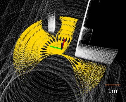
(a) (a)
(b)
(b)
(c)
(c)
(d)
Fig. 6: Simulation results of the indoor environment.(a) shows the
resulting map of our method and trajectories of all methods. The (d)
blue dot indicates the start point of all trajectories. (b) is the average Fig. 7: Simulation results of the campus environment. The figure
explored volumes vs. time.(c) is the average traveling distances vs. shares the same layout as Fig.6.
time. (d) is the average runtime vs. time.
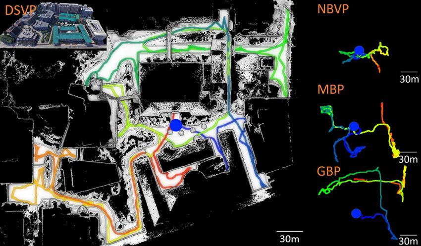
For GBP and MBP, we observe that they have difficulty in
As can be seen, GBP and MBP are both capable of exploring triggering the relocation mode when the environment is open.
the entire area while NBVP can only cover a limited area After traveling 2636m in 1427s in the campus environment
because it has limitations in relocating the vehicle. Our and 4952m in 2830s in the garage environment, our method
method covers the complete space. Fig. 6b and 6c compare finishes the exploration. Note that the other methods take a
the average explored volume and traveling distance of all longer exploration time in the campus environment, but the
methods. Our method completes the exploration after travel- resulting traveling distance is less than ours. This is due to
ing 1384m over 912s. It can be seen that GBP can not cover long planning time and rotations in redundant back-and-forth
the whole space every time, causing the average volume motion to slow down the driving speed.
much less than our methods. GBP and MBP are often trapped Tables II and III compares the exploration efficiency
in dead end areas. Our method can cover the space fully in and algorithm runtime between our method and the other
all evaluated runs. methods. In Table II, (m3 /s) is the average value of the
Fig. 7 and 8 demonstrate the results for campus and efficiency of all runs. The efficiency of one run is defined
garage environments. From the best trajectories of NBVP, as the average explored volume per second in that run.
GBP and MBP in Fig. 7a and Fig. 8a, we can see that r is the relative efficiency compared to our method. The
these methods are unable to cover the entire environment. average runtime of our method is the smallest in all evaluated
TABLE II: Comparison of exploration efficiency TABLE III: Comparison of planning time
NBVP MBP GBP DSVP Average Runtime (s) CPU Load (%)
r r r r NBVP MBP GBP DSVP NBVP MBP GBP DSVP
Indoor 1.2 0.18 3.3 0.49 3.6 0.53 6.8 1.0 Indoor 2.48 1.97 1.46 0.81 47 27 26 19
Campus 11.1 0.33 11.7 0.35 12.1 0.36 33.6 1.0 Campus 2.41 3.31 3.08 1.03 37 47 33 19
Garage 0.9 0.05 2.8 0.17 6.0 0.37 16.4 1.0 Garage 1.84 1.71 2.33 0.72 40 22 44 17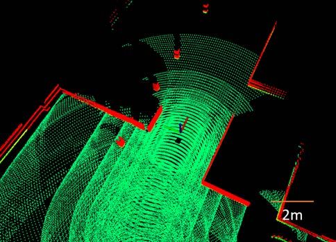
Fig. 9: Experiment vehicle platform
                              (a)

                                                                   The system uses our prior method for state estimation as well
                                                                   as mapping explored areas [24]. The system also incorporates
                                                                   navigation modules from our benchmark environment, e.g.
                                                                   collision avoidance, terrain traversability analysis, way-point
                                                                   following, as the mid-layer. During exploration, the collision
                                                                   avoidance module [23] further prevents collisions and war-
                              (b)
                                                                   rants safety. Our exploration algorithm is at the top layer in
                                                                   the system, running on a computer with a 4.1GHz i7 CPU.
                                                                      The experiment is conducted in an outdoor environment
                                                                   at the university campus as shown in Fig. 10. The en-
                                                                   vironment includes several intersections, dead ends and
                                                                   trees. Fig. 10a gives the final trajectories of all methods.
                                                                   The trajectory of NBVP reveals considerable back-and-forth
                              (c)                                  behaviors through the whole process. One issue of MBP
                                                                   and GBP is that they have trouble handling thin structures
                                                                   such as tree branches. The reason is relevant to what is
                                                                   mentioned above that they extend the global RRG randomly
                                                                   in the relocation mode. Due to the fact that the sampled
                                                                   viewpoints in relocation mode are distant from the robot,
                                                                   lidar scan data can miss the thin structures causing the
                              (d)                                  places to be considered traversable. As the vehicle navigates
Fig. 8: Simulation results of the garage environment. The figure   closer, the sampled viewpoints are not effectively eliminated
shares the same layout as Fig.6.                                   from the global graph, causing the vehicle to be trapped
environments. With dynamically-expanded RRT, our method            around trees. In contrast, our method actively eliminates
does not need to regenerate a new dense local tree every           edges on the local RRT and global graph that interfere with
time, which saves much time especially when the space is           obstacles. This gives our method the advantage of dealing
open. Further, our method leverages the global frontiers with      with thin structures in the environment from which laser
the global graph to eliminate the need of a dense global           returns are inconsistent. Fig. 10b and Fig. 10c compare the
graph - the method uses a relatively sparse global graph           explored volume and traveling distance of four methods.
to navigate to the vicinity of the global frontiers and then       NBVP spends 2160s covering 8677m3 while our method
uses the global frontiers to guide the vehicle further. While      spends 322s covering the same space. GBP spends 1984s
for GBP and MBP, they incrementally add more nodes to              covering 15192m3 which only takes 843s for our method.
the global RRG by randomly sampling viewpoints in the              MBP explores almost the same space as our method while
relocation mode, which leads to a dense global RRG. In             the time is almost double. Fig. 10d shows the runtime of each
addition, GBP and MBP need to compute the reward of                method. The average runtime for NBVP is 2.02s, for GBP
each viewpoint in the global RRG continuously to decide            is 3.9s and for MBP is 1.05s. The average runtime for our
which one has the highest reward, which takes considerable         method is 1.4s. Even though our runtime is slightly longer
computation time. Our method, however, neglects the reward         than MBP, the variation is much smaller as one can see a
of the viewpoints in the global graph and only checks if           large spike in the runtime of MBP.
a viewpoint can observe a given frontier, as described in
                                                                                        VI. C ONCLUSION
Algorithm 3, which takes considerably less time.
                                                                     We propose a method for efficiently exploring environ-
B. Physical Experiment                                             ments at a high-degree of convolution. By switching between
   We conduct experiments using the vehicle platform in            exploration stage and relocation state, our method is able to
Fig. 9. The vehicle is equipped with a Velodyne Puck lidar,        cover the entire environment. The method dynamically ex-
a camera at 640 × 360 resolution, and a MEMS-based IMU.            pand the local RRT and global graph, and use hybrid frontiers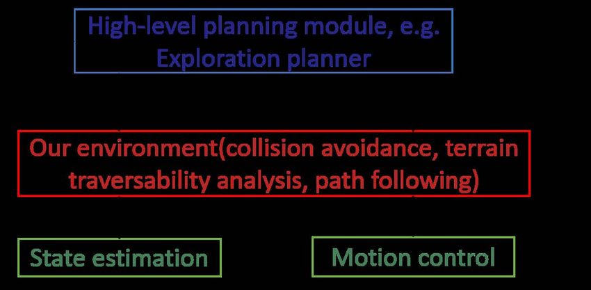
environment exploration, and structural reconstruction,” IEEE Robotics
                                                                                        and Automation Letters, vol. 2, no. 3, pp. 1680–1687, 2017.
                                                                                  [6]   B. Fang, J. Ding, and Z. Wang, “Autonomous robotic exploration based
                                                                                        on frontier point optimization and multistep path planning,” IEEE
                                                                                        Access, vol. 7, pp. 46 104–46 113, 2019.
                                                                                  [7]   C. Dornhege and A. Kleiner, “A frontier-void-based approach for
                                                                                        autonomous exploration in 3D,” Advanced Robotics, vol. 27, no. 6,
                                                                                        pp. 459–468, 2013.
                                                                                  [8]   L. Heng, A. Gotovos, A. Krause, and M. Pollefeys, “Efficient visual
                                                                                        exploration and coverage with a micro aerial vehicle in unknown
                                                                                        environments,” in IEEE International Conference on Robotics and
                                                                                        Automation (ICRA), Seattle, WA, May 2015.
                                     (a)                                          [9]   T. Cieslewski, E. Kaufmann, and D. Scaramuzza, “Rapid exploration
                                                                                        with multi-rotors: A frontier selection method for high speed flight,” in
                                                                                        IEEE/RSJ International Conference on Intelligent Robots and Systems
                                                                                        (IROS), Vancouver, Canda, Sept. 2017.
                                                                                 [10]   M. Selin, M. Tiger, D. Duberg, F. Heintz, and P. Jensfelt, “Efficient
                                                                                        autonomous exploration planning of large-scale 3-d environments,”
                                                                                        IEEE Robotics and Automation Letters, vol. 4, no. 2, pp. 1699–1706,
                                                                                        2019.
                                                                                 [11]   C. Wang, H. Ma, W. Chen, L. Liu, and M. Q.-H. Meng, “Efficient
                                     (b)                                                autonomous exploration with incrementally built topological map
                                                                                        in 3-d environments,” IEEE Transactions on Instrumentation and
                                                                                        Measurement, vol. 69, no. 12, pp. 9853–9865, 2020.
                                                                                 [12]   M. Dharmadhikari, T. Dang, L. Solanka, J. Loje, H. Nguyen,
                                                                                        N. Khedekar, and K. Alexis, “Motion primitives-based agile ex-
                                                                                        ploration path planning for aerial robotics,” in IEEE International
                                                                                        Conference on Robotics and Automation (ICRA), Paris, France, May
                                                                                        2020.
                                                                                 [13]   T. Dang, M. Tranzatto, S. Khattak, F. Mascarich, K. Alexis, and
                                     (c)                                                M. Hutter, “Graph-based subterranean exploration path planning using
                                                                                        aerial and legged robots,” Journal of Field Robotics, vol. 37, no. 8,
                                                                                        pp. 1363–1388, 2020.
                                                                                 [14]   R. Reinhart, T. Dang, E. Hand, C. Papachristos, and K. Alexis,
                                                                                        “Learning-based path planning for autonomous exploration of subter-
                                                                                        ranean environments,” in IEEE International Conference on Robotics
                                                                                        and Automation (ICRA), Paris, France, May 2020.
                                                                                 [15]   T. Chen, S. Gupta, and A. Gupta, “Learning exploration policies for
                                                                                        navigation,” in Proceedings of Seventh International Conference on
                                    (d)                                                 Learning Representations (ICLR), New Orleans, LA, May 2019.
Fig. 10: Results of the experiment in an outdoor environment. (a)                [16]   F. Niroui, K. Zhang, Z. Kashino, and G. Nejat, “Deep reinforcement
is the resulting map of our method and trajectories of all methods.                     learning robot for search and rescue applications: Exploration in
The blue dot indicates the start point of all trajectories. (b) is the                  unknown cluttered environments,” IEEE Robotics and Automation
explored volumes vs. time.(e) is the traveling distances vs. time. (f)                  Letters, vol. 4, no. 2, pp. 610–617, 2019.
                                                                                 [17]   T. Kollar and N. Roy, “Trajectory optimization using reinforcement
is the runtime vs. time.
                                                                                        learning for map exploration,” The International Journal of Robotics
                                                                                        Research, vol. 27, no. 2, pp. 175–196, 2008.
to guide the expansion. We evaluate the method in a real                         [18]   M. Kulich, J. Faigl, and L. Přeučil, “On distance utility in the
outdoor environment and three simulation environments, i.e.                             exploration task,” in IEEE International Conference on Robotics and
indoor, campus and garage environments in the benchmark                                 Automation (ICRA), Shanghai, China, May 2011.
                                                                                 [19]   M. Kulich, J. Kubalík, and L. Přeučil, “An integrated approach to goal
environment that we develop to facilitate development of                                selection in mobile robot exploration,” Sensors, vol. 19, no. 6, 2019.
autonomous navigation systems. Our method is compared to                         [20]   S. Karaman and E. Frazzoli, “Sampling-based algorithms for optimal
three state-of-art methods. The results show that our method                            motion planning,” The International Journal of Robotics Research,
                                                                                        vol. 30, no. 7, pp. 846–894, 2011.
covers the space twice as fast as the other methods while                        [21]   A. Hornung, K. M. Wurm, M. Bennewitz, C. Stachniss, and W. Bur-
taking less computation.                                                                gard, “Octomap: An efficient probabilistic 3d mapping framework
                                                                                        based on octrees,” Autonomous robots, vol. 34, no. 3, pp. 189–206,
                                                                                        2013.
                             R EFERENCES                                         [22]   E. J. Keogh and M. J. Pazzani, “Derivative dynamic time warping,”
                                                                                        in Proceedings of the 2001 SIAM international conference on data
 [1] S. M. Lavalle, “Rapidly-exploring random trees: A new tool for path
                                                                                        mining. SIAM, 2001, pp. 1–11.
     planning,” Tech. Rep., 1998.
                                                                                 [23]   J. Zhang, C. Hu, R. G. Chadha, and S. Singh, “Falco: Fast likelihood-
 [2] A. Bircher, M. Kamel, K. Alexis, H. Oleynikova, and R. Siegwart,                   based collision avoidance with extension to human-guided navigation,”
     “Receding horizon" next-best-view" planner for 3D exploration,” in                 Journal of Field Robotics, vol. 37, no. 8, pp. 1300–1313, 2020.
     IEEE International Conference on Robotics and Automation (ICRA),            [24]   J. Zhang and S. Singh, “Laser-visual-inertial odometry and mapping
     Stockholm, Sweden, May 2016.                                                       with high robustness and low drift,” Journal of Field Robotics, vol. 35,
 [3] B. Yamauchi, “A frontier-based approach for autonomous exploration,”               no. 8, pp. 1242–1264, 2018.
     in Proceedings 1997 IEEE International Symposium on Computational
     Intelligence in Robotics and Automation, 1997, pp. 146–151.
 [4] D. Holz, N. Basilico, F. Amigoni, and S. Behnke, “Evaluating the ef-
     ficiency of frontier-based exploration strategies,” in 41st International
     Symposium on Robotics (ISR) and 6th German Conference on Robotics
     (ROBOTIK), 2010, pp. 1–8.
 [5] Z. Meng, H. Qin, Z. Chen, X. Chen, H. Sun, F. Lin, and M. H. Ang, “A
     two-stage optimized next-view planning framework for 3-d unknown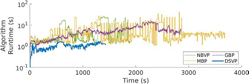
You can also read