EDUCE: Explaining model Decisions through Unsupervised Concepts Extraction
←
→
Page content transcription
If your browser does not render page correctly, please read the page content below
EDUCE: Explaining model Decisions through
                                                    Unsupervised Concepts Extraction

                                                             Diane Bouchacourt                           Ludovic Denoyer
                                                            Facebook AI Research                       Facebook AI Research
                                                              dianeb@fb.com                              denoyer@fb.com
arXiv:1905.11852v1 [cs.LG] 28 May 2019

                                                                                       Abstract

                                                  With the advent of deep neural networks, some research focuses towards un-
                                                  derstanding their black-box behavior. In this paper, we propose a new type of
                                                  self-interpretable models, that are, architectures designed to provide explanations
                                                  along with their predictions. Our method proceeds in two stages and is trained
                                                  end-to-end: first, our model builds a low-dimensional binary representation of any
                                                  input where each feature denotes the presence or absence of concepts. Then, it
                                                  computes a prediction only based on this binary representation through a simple
                                                  linear model. This allows an easy interpretation of the model’s output in terms of
                                                  presence of particular concepts in the input. The originality of our approach lies
                                                  in the fact that concepts are automatically discovered at training time, without the
                                                  need for additional supervision. Concepts correspond to a set of patterns, built
                                                  on local low-level features (e.g a part of an image, a word in a sentence), easily
                                                  identifiable from the other concepts. We experimentally demonstrate the relevance
                                                  of our approach using classification tasks on two types of data, text and image, by
                                                  showing its predictive performance and interpretability.

                                         1   Introduction
                                         As the scope of application of deep neural networks has greatly widened, two main directions of
                                         research have been developed to make their behavior more understandable by humans. The first
                                         direction aims at developing algorithms that have the ability to explain a posteriori any black-box
                                         model [20]. The second direction proposes new models and architectures that exhibit predictive
                                         performance close to deep learning ones, while being interpretable by the users (see for example
                                         [7, 27, 2, 19]). In both these research directions, producing explainable or interpretable models usually
                                         relies on two core components: (i) First, the interpretation or explanation has to be grounded over
                                         concepts, that are, notions that make sense to a human. For instance, to explain an image classification
                                         prediction, an explanation/interpretation at the pixel-level (e.g. based on the importance of each pixel
                                         in the prediction) would be difficult to parse. Therefore, existing approaches typically use higher-level
                                         features like super-pixels [20]. (ii) Second, the interpretation/explanation is supported by only a few
                                         human-understandable concepts, since grounding the decision on too many parameters would harden
                                         the interpretation. In many existing methods, the list of concepts on which the prediction is grounded
                                         is given to the model as additional knowledge (e.g human labels that define concepts [11]). This has
                                         two important drawbacks: It requires an additional effort to manually label data at the concept-level
                                         and it may introduce bias in the interpretation. Indeed, a priori human-defined concepts have no
                                         guarantees to be relevant for the given task.
                                         In this article, we propose a new deep learning model which objective is to be self-interpretable
                                         by automatically discovering relevant concepts, thus avoiding the need for extra labeling or the
                                         introduction of any artificial bias. Furthermore, the proposed model uses a very general architecture
                                         based on convolutions, both for text and image data. As a consequence, our method is easily

                                         Preprint. Under review.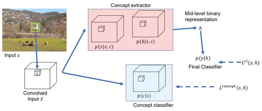
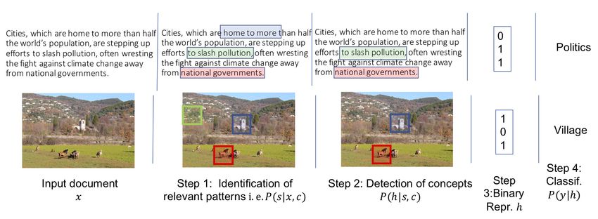
Figure 1: Our inference process, we show two examples: one for text data (above) and one for
image data (below). Patterns are identified in the input as potentially capturing some concepts – 3
concepts in these examples. Then only relevant patterns are kept to build a low-dimensional binary
representation that denotes the presence or absence of concepts. This binary representation is used
with a linear classifier (without bias) resulting in simple interpretable decision rules.

applicable to any new dataset. To do so, we rely on two main principles: i) our model learns to
represent any input as a binary vector where each feature corresponds to a concept being absent or
present in that input and ii) it computes its final prediction only using this binary representation. This
allows an interpretation of the model’s prediction using only the appearance of concepts, and results
in very simple decision rules. The presence of a concept is defined by the appearance of a local
pattern that must be easily identifiable as belonging to an homogeneous set of patterns. We enforce
this through a concept identification constraint, which facilitates the interpretation of the extracted
concepts. Our contributions are threefold: i) We propose a new deep self-interpretable model that
is able to predict solely from the presence or not of concepts in the input, where the concepts are
discovered without supervision. ii) We instantiate this model for both images and text through
convolutional neural networks and describe how its parameters are efficiently learned with stochastic
optimization. iii) We analyze the quality of the learned models on different text categorization and
image classification datasets, and show that our model reaches good classification accuracy while
extracting meaningful concepts.
The paper is organized as follows: in Section 2 we describe the general idea of our approach and
explain how it can be casted as a learning problem optimized with stochastic optimization techniques.
We experimentally train our model and analyze the results for both images and text in Section 3 and
4. In Section 5, we connect our method to existing interpretable models.

2     The EDUCE model

In this paper, we tackle multi-class classification tasks but our model can be easily extended to any
supervised problem such as regression or multi-label classification. We consider a training dataset D
of inputs {x1 , ...., xN }, xn ∈ X and corresponding labels {y1 , ..., yN }, yn ∈ Y. The goal is to learn
a predictive function f (x) : X → Y that exhibits high classification performance, while being easily
understandable by humans.

2.1   Principles

The general idea of our approach is the following: classical (deep learning) models take as input
low-level features describing the inputs (e.g pixels, words) and directly provide a high-level output,
such as a category label y. The final prediction is entirely based on complex computations over
low-level input features, which renders the interpretation of the model hard to parse for a human.
Even if Deep Neural Network (DNN) based models build intermediate representations, these are
often high-dimensional and not constrained to extract meaningful information.

                                                    2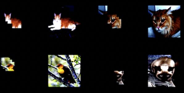
Our model, called EDUCE for Explaining model Decisions through Unsupervised Concepts Extrac-
tion relies on two main principles:

       • Low-dimensional Binary Representation for Classification: EDUCE builds a mid-level
         representation of any input in the form of a low-dimensional binary vector. Each binary
         feature denotes the presence or absence of different concepts in the input x and is computed
         by extracting local patterns or subparts of the input (see Figure 1). The output is computed
         based on this binary representation allowing a quick interpretation of the decision.1
       • Concepts Identification: Since the training dataset does not contain any mid-level labels,
         the extraction of meaningful concepts is unsupervised but constrained through the concept
         identification criterion that ensures that all the patterns extracted for each concept carry a
         common semantics, thus allowing an easier interpretation.

These two principles are captured through three main components learned simultaneously: (i) the
concept extractor is in charge of identifying if and where a concept appears in the input, (ii) the final
classifier computes the final prediction based on the absence/presence of the concepts and (iii) the
concept classifier ensures that concepts are homogeneous and identifiable from each others.

2.2   Concept extraction and final prediction

Let us consider a set C of C concepts. The concept extractor builds an intermediate binary representa-
tion h ∈ {0; 1}C of the input x, where each value hc denotes the presence or absence of concept c in
x. Therefore, the concept extractor replaces the first layers in classical DNN architectures, such that h
is low-dimensional and discrete (binary in our case). We build h through a stochastic process in two
steps: i) first for each concept c, patterns that are the more likely to correspond to each concept are
identified (step 1 Figure 1) and ii) each extracted pattern is used to decide on the absence or presence
of c into x (step 2 Figure 1) giving the binary representation (shown in step 3 Figure 1).
Let us define Sx as the set of all local patterns s in x, for example a set of patches in an image.
We denote pγ (s|x, c) ∀s ∈ S Px the probability that the pattern contained in s is the most relevant to
concept c in x i.e. such that s∈Sx pγ (s|x, c) = 1, and γ are the parameters of the distribution. Now
let us denote pα (hc = 1|s, c) the probability, parameterized by α, that the extracted pattern s triggers
the presence of concept c. The intermediate representation h of x is obtained by two consecutive
sampling steps:
                                ∀c, sc ∼ pγ (s|x, c), hc ∼ pα (hc |sc , c).                           (1)

The final decision is solely computed from the intermediate representation h. We use a linear
classifier without bias to rely on its weights for its interpretation: for each category y, each concept
c is associated with a weight denoted δy,c . The final score is computed by summing the weights
of concepts identified into the input, i.e. for which hc = 1. We obtain thePprobability pδ (y|h),
parameterized by δ, through a softmax function such that pδ (y|h) = softmax c δy,c hc .2

2.3   Concepts identification

Since h is a binary representation of x, our method is very close to sparse-coding techniques [17] and
does not have the incentive to extract meaningful information. Without any additional constraint, it
would be difficult or even impossible to interpret the concepts discovered by the model. Indeed, due
to the combinatorial nature of the mid-level representation h, the model can easily find combinations
of patterns that allow good classification accuracy, without extracting meaningful patterns. Let us
denote {sc }c∈C the patterns extracted by the concept extractor for each concept. It is necessary to
ensure that, for any concept c, all extracted sc share common semantics, and that the semantics
carried by patterns in concept c is different than the one carried by patterns in another concept c0 .
This constraint is enforced in EDUCE by jointly learning a multiclass concept classifier able to
classify the pattern sc in x as belonging to concept c, thus defining the categorical distribution pθ (c|s)
    1
      In our case, the classifier is a linear model without bias, and thus final score is a weighted sum of the
concepts appearing in the input.
    2
      Note that, for sake of clarity, we use an approximative notation as the softmax function considers the scores
of all possible categories y ∈ Y.

                                                        3
Algorithm 1: – Training Algorithm.
Given a training datapoint (x, y):
1 Sample s and h following the process described in Equation 1.
P
2 Update δ with ∇δ L = ∇δ log softmax c δy,c hc
T
3 Update θ with ∇θ L = λc ∇θ log softmaxθc sc
4 Update α and γ with Reinforcement Learning:
∇α L = Es,h∼pγ ,pα [(− log pδ (y|h) + λc Lconcept (θ, s, h) + λL1 |h|)∇α log pα (hc |sc , c)] (4)
concept
∇γ L = Es,h∼pγ ,pα [(− log pδ (y|h) + λc L (θ, s, h) + λL1 |h|)∇γ log pγ (sc |x, c)] (5)
where θ are its parameters. This classifier is learned on patterns responsible for each concept’s
appearance in the input. Therefore, the concept classification loss is the cross-entropy loss, only
considering concepts c appearing in x (i.e such that hc = 1).
X
Lconcept (θ, s, h) = − hc log pθ (c|sc ). (2)
c
Another way to obtain consistent patterns would be to add a sparsity constraint on the number
of concepts present in any input, preventing the use of combinations of patterns to have good
classification accuracy. Therefore, we consider adding a L1 -norm constraint on the number of
concepts that are present for a given input example. Nonetheless, we experimentally demonstrate that
the L1 constraint is not sufficient, and can harm final performance by making the representation h
coarser. On the opposite, our concept classifier is necessary and sufficient: Lconcept (θ, s, h) depends
on the number of concepts present hence sparsity is encouraged. However, if discovered concepts are
consistent and easy to identify, Lconcept (θ, s, h) can be low without harming task performance.
2.4 Objective function and learning algorithm
Our objective function mixes the final classification cross-entropy and the concept classifier loss, as:
L = L(θ, γ, α, δ, x, y) = Es,h∼pγ ,pα [− log pδ (y|h) + λc Lconcept (θ, s, h) + λL1 |h|]. (3)
where s and h are sampled as in Equation 1, λc controls the strength of the concept identification
w.r.t. the final prediction, λL1 guides the strengh of the sparsity constraint and || denotes the L1 -norm.
The learning algorithm optimizes the parameters of the distributions pθ (c|s), pγ (s|x, c), pα (h|s, c)
and pδ (y|h). As the explicit computation of the expectation involves expensive summations over all
possible values of h and s we resort to Monte-Carlo approximations of the gradient. This is a classic
method in the Reinforcement Learning [25]. The resulting learning algorithm is given in Algorithm 1
and the gradient derivation is provided in Supplementary Material.3 Note that the learning can be
efficiently implemented for a large variety of architectures over batches, using one GPU per run. Our
code for the text and image experiments will be released upon acceptance.
3 Text classification experiments
Setting We experiment on the DBpedia ontology classification dataset and the AGNews topic
classification dataset [28]. The DBpedia ontology classification dataset was constructed by picking
14 non-overlapping categories from DBpedia 2014 [14]. We subsample 56, 000 examples of the
train dataset for training, and 56, 000 for validation. For testing, we subsample 7, 000 of the 70, 000
examples in the test dataset (using stratified sampling). The AGNews topic classification dataset
was constructed from the AG dataset’s 4 largest categories. We divide the training set into two sets:
84, 000 training samples and 24, 000 validation samples. We test on the full test dataset composed
of 7, 600 samples. We use pre-trained word vectors trained on Common Crawl [8], and keep them
fixed. We consider patterns s as all sets composed of 3 consecutive words.4 Therefore, sampling a
pattern is equivalent to the sampling of its start word. For comparison, we train a non-interpretable
“Classic" model that uses a Bidirectional LSTM, while EDUCE is based on convolutional layers as
3
We use the average loss as control variate.
4
We considered flexible number of words in the patterns but performance were poorer, we consider this as
direction for future research.
4A Posteriori
Model λc λL1 Final Acc. (%) Concept Acc. (%) Sparsity
Concept Acc. (%)
DBPedia
Baseline 0.00 0.00 94.3 ± 0.1 11.4 ± 0.8 65 ± 1.5 6.75 ± 0.1
Baseline 0.00 0.01 94.7 ± 0.2 11 ± 1.3 67 ± 1.6 5.6 ± 0.2
Baseline 0.00 0.10 93.0 ± 0.2 12 ± 1.8 88 ± 1.1 1.66 ± 0.0
EDUCE 0.10 0.00 93.6 ± 0.3 92.9 ± 1.0 92 ± 1.1 5.4 ± 0.3
Classic 98.37 ± 0.1 N/A N/A N/A
AGNews
Baseline 0.00 0.00 87.3 ± 0.3 10.0 ± 0.8 66.8 ± 0.8 5.6 ± 0.2
Baseline 0.00 0.01 87.3 ± 0.3 10.7 ± 0.9 73 ± 1.5 3.8 ± 0.2
Baseline 0.00 0.10 83.4 ± 0.5 12 ± 1.8 95 ± 1.5 1.16 ± 0.1
EDUCE 0.10 0.00 86.2 ± 0.2 93.0 ± 0.8 91 ± 1.0 3.1 ± 0.3
Classic 90.4 ± 0.2 N/A N/A N/A
Table 1: Test performance on text classification using multiple λc and λL1 (mean ± SEM). In bold
the best comprise model. Values in red are discussed in text.
we want to use a general architecture that works on multiple data types. We monitor final prediction
accuracy on the validation set and report results on the test set. For each set of hyperparameters, we
run 5 different random seeds. We explore three different number of concepts: C = 5, C = 10 and
C = 20. Details on the range of hyperparameters, the training procedure and size of the architecture
is in supplementary material Section 8.
Quantitative analysis Table 1 reports the performance on the DBPedia dataset and AGNews dataset
for C = 10 concepts. We report the final accuracy (Final Acc.) over the task, the accuracy of the
concept classifier on the test data (Concept Acc.). Naturally, Concept Acc. should be low for models
with λc = 0. Therefore, we also compute an a posteriori concept accuracy: after training, for each
model, we gather the concepts patterns it detects (hc = 1) on the test data. We separate the patterns
into two sets (training and testing, note that these are both generated from the test data). For each
model, we train a new concept classifier a posteriori on the model’s patterns and report the a posteriori
concept classifier performance (A Posteriori Concept Acc.). We also report the average number of
concept that are detected as present (i.e. hc = 1) per input (Sparsity). We tried different values of λc
and λL1 , and the combination of the two, our method is defined by values λc > 0). We show here the
most relevant to our analysis, complete results are available in the supplementary Section 8.3.1. For
all metrics we report the mean and standard error of the mean (SEM) over the training random seeds.
First, looking at the performance of the “Classic" model, we see that encoding the input into a
low-dimensional binary vector only reduces the accuracy of a few percent (from 98.37% to ∼ 94%
on DBPedia and 90.4% to ∼ 86% on AGNews dataset). This means that classifying by identifying
relevant patterns is an efficient approach. As expected with λc = 0, patterns extracted for each concept
are not homogeneous as a posteriori concept accuracy is low (65% and 66.8% for DBPedia and
AGNews respectively). Adding our concept classifier (λc > 0) greatly improves the concept accuracy
without significative loss on final accuracy. EDUCE obtains 93.6% (resp. 86.2%) classification
performance with 92.9% (resp. 93.0%) concept accuracy on DBPedia (resp. AGNews).
Using only a sparse constraint λL1 > 0 with λc = 0 results in a much lower concept accuracy,
meaning that patterns are less consistent within a concept. The only exception is with λL1 = 0.1 but
this achieved at the expense of final classifier’s performance that drops significatively on AGNews.
To explain this, note that on the AGNews dataset, the number of concept C = 10 is larger than the
number of categories (4 categories) so a simple solution to obtain high concept accuracy is to map
one concept per category. Indeed, the model only using L1 -norm constraint without our concept
classifier has an average of 1.16 concept present per input, and supplementary Figure A.7 shows that
this corresponds to mapping one concept per class. This makes the final performance go down to
83.4% as the representation of the input is coarser. On the opposite, our model does not suffer from
this: we achieve with λc = 0.1 a final performance of 86.2% with an a posteriori concept accuracy of
91% showing that concepts are consistent, yet maintaining on average 3.1 concepts present per input.
Note that adding the L1 constraint to our method (λL1 > 0, λc > 0) does not improve the relevance
and consistency of discovered concepts as measured by a posteriori accuracy values, and can hurt
final performance (see Table A.5 and Figure A.6 in supplementary Section 8.3.1).
Figure 2a compares the effect of using different values of C (left is DBPedia, right is AGNews). We
see that using a smaller value results in higher concept accuracy, at the expense of final classification
performance. On the opposite, a larger value of C gives higher final classification performance,
5(a) Test performance on text data with different number of concepts C (b) Per category concept frequency.
(left is DBPedia, right is AGNews). Each line corresponds to a value Mean of Transp. stands for Mean
of C. Each marker on the lines corresponds respectively to increasing of Transportation, Educational Inst.
the value of λc . Orange line is for the “Classic" model for which stands for Educational Institution.
concept accuracy is not applicable. Shaded areas correspond to SEM.
which is expected as the binary representation is of larger size, but in poorer a posteriori concept
accuracy. Still using C = 20 concepts and λc = 0.1 we achieve 90% concept accuracy on DBPedia
and a higher final classifier performance than with 10 concepts.
Interpreting EDUCE We turn to show how EDUCE’s category prediction is easily interpretable.
The following results were generated with λc = 1 and no L1 constraint and C = 10 concepts. Table
3a shows a document from the DBPedia Dataset labeled as Natural Place, where the underlined
words correspond to the pattern extracted for different concepts. Separately, in Table 4a we show, for
each concept detected in the example of Table 3a, some patterns extracted from others test documents
(each set of 3 words is a pattern, patterns are comma-separated). This allows us to interpret the
concepts’ meaning: concept 0 maps to the notion of geographical information, concept 7 to the idea
of nature and concept 3 to the notion of municipality. We also see that the patterns extracted in
the example Natural Place in Table 3a are consistent with these interpretations. Importantly, note
that in Table 4a patterns are consistent yet come from multiple categories: for the four concepts
shown, each extracted pattern belongs to a different category. To corroborate this, Figure 2b shows
the empirical frequency of presence of each concept, per category. We see that multiple concepts
appear per category, and that concepts are shared among categories. For this setting sparsity is 2.5
(see supplementary Table A.5), i.e. on average each text input triggers 2.5 concepts. These results
show how easily the categorization of any text can be explained by the detection of multiple, relevant,
and intelligible concepts. More qualitative examples are in the supplementary Section 9.
moonie river a perennial river of the barwon catchment within the murray–darling basin is located in the
southern downs district of queensland and orana district of new south wales australia . the rivers rises south
west of dalby near braemar state forest south-east of tara in queensland and flows generally to the south-west
joined by thirteen minor tributaries before reaching its confluence with the barwon river near the village of
mogi mogi in new south wales descending 198 metres ( 650 ft ) over its 542 kilometres ( 337 mi ) course .
(a) Example of Natural Place text. Underlined set of words are patterns extracted, one color per concept.
Concept Extracted patterns
0 company on the, 9-12 located in, was built based, tract was designed, is located in, district located
in,
3 officer and president, ’ s emperor, a southern politician, of western deputy, charles school district,
served as clerk, of the minister, a joint initiative, southern downs district,
7 . monadnock is, species with, australian genus of, a horse that, ( upstream on, via mare is,
minor tributaries before,
9 around washington dc, as sub-saharan africa, new south wales, to michael jackson, is a bollywood,
is kurt austin, in avon ohio, is an american, jonathan david morris, on 25 february, in kingston
rhode,
(a) Concept examples patterns that are extracted for some test inputs. Colors match the colors used in Table 3a.
’’ stands for unknown word.
Table 4: Interpretation of a Natural Place example categorization.
64 Image classification experiments
Having assessed the relevance of our model on text data, we now turn to image data and explore if
the EDUCE model is also able to extract meaningful concepts.
Setting We tackle image classification using MNIST [13] to evaluate our approach, and results
over the dataset are given in supplementary material. To further test the relevance of the patterns
detected, we build a dataset where each image contains two randomly located of different labels.
As we consider labels 0 to 4, there are 10 possible resulting categories that are the combination
of the two digits label: (0, 1), (0, 2), ..., (3, 4). We train on 32, 000 generated images, and tested
on 32, 000 different images. We achieve test final classification performance 96% using C = 10
concepts. Figure 3 shows extracted patterns (not cherry picked) for the 10 concepts, and the categories
associated with the appearance of this concept. As in our experiments with text data, we can explain
the model behavior: the model learns to extract single digits as patterns for different concepts, that
are then combined to predict the final category.
(0,4) / (1,4) / (2,4) / (3,4) (0,1) / (1,2) / (1,3) / (1,4) (1,3) / (1,4) / (3,4) (0,1) / (0,2) / (0,3) / (0,4) / (1,4) /
(2,4)
(0,2)/(1,2)/(1,3)/(2,3)/(2,4) (0,2) / (0,3) / (0,4) / (2,3) / (2,4) (0,1) / (0,2) / (0,3) / (0,4) (0,2) / (0,3) / (2,3)
Figure 3: Samples of patterns extracted for each concept. Under each concept, we show the categories
associated with this concept
We also conduct experiments on a dataset composed of 224 × 224 RGB images split in 3 categories:
dogs, cats and birds5 in equal proportion. We train on 3, 000 images and test on 3, 000 images. We
build our model on top of a pretrained VGG-11 model [22]. Figure 2 shows extracted patterns and
associated categories. Final classification performance is 91.6% with 10 concepts. In Figure 4 we
plot extracted patterns for the 10 concepts and report in Figure 5a the weights of the final classifier.
From these two figures, we can interpret the model’s behavior: concept 8 and concept 9 show what
differentiate a dog from a cat or a bird, and support the classifier’s prediction of the dog category.
Figure 5b shows the extracted patterns on random images. We can see that our model focuses on
relevant parts of the images, similar to attention models.
Concept 0 Concept 1 Concept 2 Concept 3 Concept 4
Concept 5 Concept 6 Concept 7 Concept 8 Concept 9
Figure 4: Samples of patterns extracted for each concept in the birds-cats-dogs dataset.
5
We construct this dataset by combining random images from the Caltech Bird 200-2011 dataset [26] with
images of the cats-and-dogs Kaggle dataset [9]
7Bird
Cat
Dog
(a) Final Classifier weights, each column is a con-
cept (0 to 9, from left to right) each row a final
category. The lighter, the higher the weight is.
Concepts 6 and 7 are associated to category ’Bird’, (b) Examples of classified images (column 2 and
Concept 1 and 4 to ’Cat’ and concepts 8 and 9 to 4) and corresponding extracted patterns (column 1
’Dog’. and 3) for concept detected as present.
5 Related work
A posteriori explanations A first type of existing methods interprets an already-trained model,
typically using perturbation and gradient-based approach. The most famous method is LIME [20],
but other method exist [4, 21, 23, 24]. [3] design a model that detects input-output pairs that are
causally related. [11] propose to explain a model’s prediction by learning concept activation vectors.
However, the classifier is fixed and concepts are predefined, requiring human annotations, while we
learn both jointly and in an unsupervised and end-to-end manner.
Self-interpretable models Contrarily to the previous line of work, our work fall in the domain of
self-interpretable models. Several existing methods propose interpretable models for NLP tasks. Such
methods are specific to text data select and rationales, i.e. parts of text, on which the model bases its
prediction, see [15, 27] and very recently [5]. Moreover, they do not encourage selected rationales to
match dataset-wide instances of concepts. [7] propose visual explanations of a classifier’s decision,
while [1] use an architecture composed of an observer and a classifier, in which the classifier’s
prediction can be exposed as a binary tree structure. However, contrarily to ours, their model does not
provide a local explanation of the decision based on parts of the input. Closer to our work, [2] learn a
self-explaining classifier that takes as input a set of concepts extracted from the original input and a
relevance score for each concept. While they define a set of desiderata for what is an interpretable
concept, they simply represent the set of extracted concept as an encoding of the input and learn it
with an auto-encoding loss. Their work can be seen as a generalization of [16]. [19] extend a classic
variational auto-encoder architecture with a differentiable decision tree classifier that takes as input
the encoding of the data sample. Hence the classification is based on a binary representation of the
data as in our model. However, they methodology is different and they only experiment on image
data.
Other works Albeit not directly towards building an interpretable classifier, [10] propose an attractive-
repulsive loss which clusters the data into the different categories. [18] propose a model that learns
to define a concept by a combination of events in an environment. Our work is also close to Latent
Dirichlet Allocation (LDA) for topic models [6], yet the methodology is different: LDA learn the
parameters of a probabilistic graphical model of text generation with approximate inference.
6 Discussion and perspectives
We propose a new neural networks-based model, EDUCE, that is self-interpretable thanks to a
two-step method. First, it computes a low-dimensional binary representation of inputs that indicates
the presence of automatically discovered concepts. Each positive feature in this representation is
associated with a particular pattern in the input, and patterns extracted for one particular concept
are enforced to be identifiable by an external classifier. We experimentally demonstrate on text
categorization and image classification, using very similar architectures in both type of data, the
relevance of our approach. The EDUCE model extracts meaningful information, and provides
understandable explanation to the final user. We contemplate multiple direction for future research.
First, if supervision at the concept level was available, we could use it to ground the discovered
concepts to ‘humans’ notions, yet letting the model discover extra-concept to avoid any bias. Another
direction would be to make EDUCE output a compact representation of the classification process, e.g.
using natural language generation on top of our approach.
8References
[1] Stephan Alaniz and Zeynep Akata. XOC: explainable observer-classifier for explainable binary
decisions. CoRR, abs/1902.01780, 2019.
[2] David Alvarez Melis and Tommi Jaakkola. Towards robust interpretability with self-explaining
neural networks. In S. Bengio, H. Wallach, H. Larochelle, K. Grauman, N. Cesa-Bianchi, and
R. Garnett, editors, Advances in Neural Information Processing Systems 31, pages 7775–7784.
Curran Associates, Inc., 2018.
[3] David Alvarez-Melis and Tommi S. Jaakkola. A causal framework for explaining the predictions
of black-box sequence-to-sequence models. In EMNLP, pages 412–421. Association for
Computational Linguistics, 2017.
[4] Sebastian Bach, Alexander Binder, Grégoire Montavon, Frederick Klauschen, Klaus-Robert
Müller, and Wojciech Samek. On pixel-wise explanations for non-linear classifier decisions by
layer-wise relevance propagation. PLoS ONE, 10(7):e0130140, 07 2015.
[5] Joost Bastings, Wilker Aziz, and Ivan Titov. Interpretable neural predictions with differentiable
binary variables, 2019.
[6] David M. Blei, Andrew Y. Ng, Michael I. Jordan, and John Lafferty. Latent dirichlet allocation.
Journal of Machine Learning Research, 3:2003, 2003.
[7] Yash Goyal, Ziyan Wu, Jan Ernst, Dhruv Batra, Devi Parikh, and Stefan Lee. Counterfactual
visual explanations, 2019.
[8] Edouard Grave, Piotr Bojanowski, Prakhar Gupta, Armand Joulin, and Tomas Mikolov. Learning
word vectors for 157 languages. In Proceedings of the International Conference on Language
Resources and Evaluation (LREC 2018), 2018.
[9] Kaggle. Kaggle dogs vs cats dataset, 2013.
[10] Kian Kenyon-Dean, Andre Cianflone, Lucas Page-Caccia, Guillaume Rabusseau, Jackie Chi Kit
Cheung, and Doina Precup. Clustering-oriented representation learning with attractive-repulsive
loss. AAAI Workshop on Network Interpretabliity for Deep Learning, 2019.
[11] Been Kim, Martin Wattenberg, Justin Gilmer, Carrie J. Cai, James Wexler, Fernanda B. Viégas,
and Rory Sayres. Interpretability beyond feature attribution: Quantitative testing with concept
activation vectors (TCAV). In Proceedings of the 35th International Conference on Machine
Learning,ICML, pages 2673–2682, 2018.
[12] Diederik Kingma and Jimmy Ba. Adam: A method for stochastic optimization. International
Conference on Learning Representations, 12 2014.
[13] Yann Lecun, Léon Bottou, Yoshua Bengio, and Patrick Haffner. Gradient-based learning applied
to document recognition. In Proceedings of the IEEE, pages 2278–2324, 1998.
[14] Jens Lehmann, Robert Isele, Max Jakob, Anja Jentzsch, Dimitris Kontokostas, Pablo N. Mendes,
Sebastian Hellmann, Mohamed Morsey, Patrick van Kleef, Sören Auer, and Christian Bizer.
DBpedia - a large-scale, multilingual knowledge base extracted from wikipedia. Semantic Web
Journal, 6(2):167–195, 2015.
[15] Tao Lei, Regina Barzilay, and Tommi Jaakkola. Rationalizing neural predictions. In Proceedings
of the 2016 Conference on Empirical Methods in Natural Language Processing, pages 107–117,
Austin, Texas, November 2016. Association for Computational Linguistics.
[16] Oscar Li, Hao Liu, Chaofan Chen, and Cynthia Rudin. Deep learning for case-based reasoning
through prototypes: A neural network that explains its predictions. In AAAI, pages 3530–3537.
AAAI Press, 2018.
[17] Julien Mairal, Francis Bach, Jean Ponce, and Guillermo Sapiro. Online dictionary learning
for sparse coding. In Proceedings of the 26th Annual International Conference on Machine
Learning, ICML ’09, pages 689–696, New York, NY, USA, 2009. ACM.
9[18] Igor Mordatch. Concept learning with energy-based models, 2018.
[19] Eleanor Quint, Garrett Wirka, Jacob Williams, Stephen Scott, and N.V. Vinodchandran. Inter-
pretable classification via supervised variational autoencoders and differentiable decision trees,
2018.
[20] Marco Tulio Ribeiro, Sameer Singh, and Carlos Guestrin. "Why Should I Trust You?":
Explaining the predictions of any classifier. In Proceedings of the 22Nd ACM SIGKDD
International Conference on Knowledge Discovery and Data Mining, KDD ’16. ACM, 2016.
[21] Avanti Shrikumar, Peyton Greenside, and Anshul Kundaje. Learning important features through
propagating activation differences. CoRR, abs/1704.02685, 2017.
[22] K. Simonyan and A. Zisserman. Very deep convolutional networks for large-scale image
recognition. CoRR, abs/1409.1556, 2014.
[23] Karen Simonyan, Andrea Vedaldi, and Andrew Zisserman. Deep inside convolutional networks:
Visualising image classification models and saliency maps. ICLR Workshop Track, 2014.
[24] Mukund Sundararajan, Ankur Taly, and Qiqi Yan. Axiomatic attribution for deep networks. In
Proceedings of the 34th International Conference on Machine Learning, ICML, 2017.
[25] Richard S. Sutton and Andrew G. Barto. Introduction to Reinforcement Learning. MIT Press,
Cambridge, MA, USA, 1st edition, 1998.
[26] C. Wah, S. Branson, P. Welinder, P. Perona, and S. Belongie. The Caltech-UCSD Birds-200-2011
Dataset. Technical Report CNS-TR-2011-001, California Institute of Technology, 2011.
[27] Mo Yu, Shiyu Chang, and Tommi S Jaakkola. Learning corresponded rationales for text
matching, 2019.
[28] Xiang Zhang and Yann LeCun. Text understanding from scratch. CoRR, abs/1502.01710, 2015.
7 Details on the learning algorithm
Algorithm 1 of the main paper shows how we compute the gradient for each of the parameter.
Specifically, when we compute the loss to be back-propagated, we tune the weight of each term. That
is, we back-propagate
X
∇δ L(θ, γ, α, δ, x, y) = (1 − λr )∇δ log softmax δy,c hc (6)
c
∇θ L(θ, γ, α, δ, x, y) = (1 − λr )λc ∇θ log softmaxθcT sc (7)
concept
∇α L(θ, γ, α, δ, x, y) = −λr Es,h∼pγ ,pα [(log pδ (y|h) + λc L (θ, s, h) (8)
+ λL1 |h|)∇α log pα (hc |sc , c)] (9)
concept
∇γ L(θ, γ, α, δ, x, y) = −λr λs Es,h∼pγ ,pα [(log pδ (y|h) + λc L (θ, s, h) (10)
+ λL1 |h|)∇γ log pγ (sc |x, c)] (11)
where λr controls the strength of the Reinforcement Learning terms w.r.t. the gradients over δ and θ,
and λs controls the strength of the gradient w.r.t. γ over the gradient w.r.t. α.
8 Details on text experiments
8.1 Detailed setting
For our experiment on text data we use the DBpedia ontology classification dataset and the AGNews
topic classification dataset both created by [28]. The DBpedia ontology classification dataset was
constructed by picking 14 non-overlapping categories from DBpedia 2014, a crowd-sourced commu-
nity effort to extract structured content from Wikipedia [14]. The train dataset has 560, 000 examples,
10among which we subsample 56, 000 examples for training, and 56, 000 for validation. For testing,
we subsample 7, 000 of the 70, 000 examples in the test dataset (using stratified sampling).
The AGNews topic classification dataset was constructed from the AG dataset, a collection of more
than 1 million news articles, by choosing 4 largest categories from the original corpus. Each category
contains 30, 000 training samples, from which we divide into two sets: 84, 000 training samples and
24, 000 validation samples. We test on the full test dataset composed of 7, 600 samples. In both
datasets the title of the abstract or article is available but we do not use it. We use pre-trained word
vectors trained on Common Crawl [8], and keep them fixed. For both datasets, the vocabulary is
built using only the most frequents 25, 000 words on the training and validation dataset. Code for
pre-processing of the datasets will be released along the code for our model.
We consider patterns s as all sets composed of 3 consecutive words. Therefore, sampling a pattern is
equivalent to the sampling of its start word resulting in an efficient sampling model. The “Classic"
model is a Bidirectional LSTM while our model is based on convolutional layers. We monitor
final prediction accuracy on the validation set and report results on the test set. For each set of
hyperparameters, we run 5 different random seeds and cross-validate hyperparameters on the average
performance across seeds. We explore three different number of concepts: C = 5, C = 10 and
C = 20, and we evidently consider each value of C separately as C directly affects the concept
classifier’s base performance. The full range of hyperparameters explored and size of the architecture
is listed in the supplementary material Section 8.
8.2 Architectures
Every word in the input is represented as an pre-trained word embedding vector. We use pre-trained
word vectors trained on Common Crawl [8] and keep them fixed. The vectors are of size 300 The
Bidirectional LSTM (BiLSTM) we use for the “Classic" model has 1 layer. The size of the hidden
state is 50. The BiLSTM processes each text input up to it maximum length, then we concatenate the
final forward and backward hidden layers together. The concatenated vector is fed to a linear layer
that returns the score over all possible categories y ∈ Y.
For our model, we consider patterns of fixed size of 3 words: for an input text x, each pattern s of x
is a combination of 3 consecutive words, therefore of size d = 3 × 300 = 900. We feed each pattern
of x to a linear layer of output size C, followed by a softmax non-linearity over the possible patterns,
for each concept. We then sample one pattern per concept at training (at test-time we take the most
probable). We then take the dot product of a weight vector αc ∈ Rd per concept with the selected
pattern, followed by a sigmoid activation function, in order to obtain the probability of that concept
being present.
8.3 Hyperparameters considered
We try the following ranges of hyperparameters λc ∈ {0, 0.01, 0.1, 1}, λL1 = {0, 0.01, 0.1}, λr ∈
{0.01, 0.1}, λs ∈ {0.01, 0.1, 1}. We use a learning rate of 0.001 and Adam optimizer [12], batches
of size 64.
8.3.1 Detailed results
Table A.5 details test performance as reported in the main paper Table 1 for all values of λL1 , λc we
tried. Figure A.6 shows final classification performance (y-axis) w.r.t. concept accuracy performance
a posteriori (x-axis) on the two text datasets considered (left is DBPedia, right is AGNews). Each
marker on the lines corresponds respectively to increasing the value of λc in {0, 0.01, 0.1, 1}. Each
line corresponds to a different value of the sparsity constraint parameter λL1 . The horizontal orange
lines denotes the “Classic" model classification performance (its concept classification performance
is not computable as it does not rely on the binary representation h). Shaded areas denotes standard
error of the mean (SEM) over the random training seeds. Both the table and figure illustrate the clear
trade-off between final classification performance and concept consistency, where concept accuracy
performance of 99% results in a much lower final accuracy. We also see that adding the L1 constraint
to our method (λL1 > 0, λc > 0) does not improve much in terms of obtaining meaningful, consistent
concepts (as per concept a posteriori accuracy values), and even hurt final performance.
11Figure A.6: Test performance on text data (left is DBPedia, right is AGNews) with C = 10 concepts.
Each marker on the lines corresponds respectively to increasing the value of λc . Each line corresponds
to a different value of the sparsity constraint parameter λL1 . Orange line is for the “Classic" model
for which concept accuracy is not applicable.
A Posteriori
Model λc λL1 Final Acc. (%) Concept Acc. (%) Sparsity
Concept Acc. (%)
DBPedia
Baseline 0.00 0.00 94.3 ± 0.1 11.4 ± 0.8 65 ± 1.5 6.75 ± 0.1
Baseline 0.00 0.01 94.7 ± 0.2 11 ± 1.3 67 ± 1.6 5.6 ± 0.2
Baseline 0.00 0.10 93.0 ± 0.2 12 ± 1.8 88 ± 1.1 1.66 ± 0.0
EDUCE 0.01 0.00 94.3 ± 0.3 80 ± 1.5 78 ± 1.5 6.5 ± 0.1
EDUCE 0.01 0.01 94.3 ± 0.2 81 ± 1.5 79 ± 1.6 5.6 ± 0.2
EDUCE 0.01 0.10 93.0 ± 0.2 93 ± 1.7 93 ± 1.9 1.64 ± 0.1
EDUCE 0.10 0.00 93.6 ± 0.3 92.9 ± 1.0 92 ± 1.1 5.4 ± 0.3
EDUCE 0.10 0.01 93.7 ± 0.3 93.9 ± 0.7 92.6 ± 0.8 4.4 ± 0.3
EDUCE 0.10 0.10 93.2 ± 0.2 93.3 ± 0.9 93 ± 1.0 1.59 ± 0.0
EDUCE 1.00 0.00 93.3 ± 0.2 98.8 ± 0.1 98.3 ± 0.1 2.5 ± 0.1
EDUCE 1.00 0.01 92.8 ± 0.2 98.6 ± 0.3 98.0 ± 0.4 2.36 ± 0.1
EDUCE 1.00 0.10 91 ± 1.3 98.3 ± 0.4 97.8 ± 0.5 1.54 ± 0.0
Classic 98.37 ± 0.1 N/A N/A N/A
AGNews
A Posteriori
Model λc λL1 Final Acc. (%) Concept Acc. (%) Sparsity
Concept Acc. (%)
Baseline 0.00 0.00 87.3 ± 0.3 10.0 ± 0.8 66.8 ± 0.8 5.6 ± 0.2
Baseline 0.00 0.01 87.3 ± 0.3 10.7 ± 0.9 73 ± 1.5 3.8 ± 0.2
Baseline 0.00 0.10 83.4 ± 0.5 12 ± 1.8 95 ± 1.5 1.16 ± 0.1
EDUCE 0.01 0.00 87.0 ± 0.4 77 ± 1.1 74 ± 1.0 5.2 ± 0.1
EDUCE 0.01 0.01 85.8 ± 0.5 82.2 ± 0.5 79.3 ± 0.7 3.25 ± 0.1
EDUCE 0.01 0.10 83.8 ± 0.2 98.0 ± 0.1 97.1 ± 0.2 1.16 ± 0.0
EDUCE 0.10 0.00 86.2 ± 0.2 93.0 ± 0.8 91 ± 1.0 3.1 ± 0.3
EDUCE 0.10 0.01 85.9 ± 0.3 94.2 ± 0.4 91.9 ± 0.5 2.2 ± 0.1
EDUCE 0.10 0.10 83.3 ± 0.7 98.3 ± 0.3 97.3 ± 0.4 1.19 ± 0.0
EDUCE 1.00 0.00 84.5 ± 0.2 98.5 ± 0.3 97.6 ± 0.3 1.7 ± 0.2
EDUCE 1.00 0.01 83.7 ± 0.8 98.7 ± 0.3 98.0 ± 0.4 1.4 ± 0.2
EDUCE 1.00 0.10 80 ± 1.8 98.8 ± 0.3 98.1 ± 0.4 1.06 ± 0.0
Classic 90.4 ± 0.2 N/A N/A N/A
Table A.5: Detailed reporting of test performance on text classification using multiple λc and λL1 . In
bold the best comprise model. Values in red are discussed in text.
Figure A.7b shows that the model only using L1 -norm constraint without our concept classifier maps
one concept per class. This is not an interesting solution, and makes the final performance goes down
12(a) Our model: λc = 0.1, λL1 = 0
(b) Strong L1 constraint baseline: λc = 0, λL1 = 0.1
Figure A.7: Comparing the frequency of concept per category for our model (in (a)) and the L1
baseline (in (b)), when the number of concept is larger than the number of categories.
to 83.4% as the representation of the input is coarser. On the opposite, our model does not suffer
from this and construct a set of concepts that are shared among the possible categories, as shown by
Figure A.7a.
Figure A.8 show the final’s classifier weights δ corresponding to the frequency of concept Figure 2b
in the main paper.
Figure A.8: Weights δ corresponding to the frequency of concept Figure 2b in the main paper.
139 Additional qualitative examples on DBPedia
Tables A.6 and A.7 show more qualitative examples on DBPedia, with the same parameters as
reported in the main paper. Table A.6 shows examples of text for each category, and the patterns
extracted. Table A.7 shows per concept, examples of pattern extracted across the different categories.
Colors between the two tables correspond.
Category Text and patterns
Company transurban manages and develops urban toll road networks in australia
and north america . it is a top 50 company on the australian securities
exchange ( asx ) and has been in business since 1996 . in australia
transurban has a stake in five of sydney ’ s nine motorways and in
melbourne it is the full owner of citylink which connects three of the city ’
s major freeways . in the usa transurban has ownership interests in the
495 express lanes on a section of the capital beltway around washington
dc .
Animal the red-necked falcon or red-headed merlin ( falco chicquera ) is a bird of
prey in the falcon family . this bird is a widespread resident in india and
adjacent regions as well as sub-saharan africa . it is sometimes called
turumti locally . the red-necked falcon is a medium-sized long-winged
species with a bright rufous crown and nape . it is on average 30–36 cm
in length with a wingspan of 85 cm . the sexes are similar except in size
males are smaller than females as is usual in falcons .
Plant astroloma is an endemic australian genus of around 20 species of flower-
ing plants in the family ericaceae . the majority of the species are endemic
in western australia but a few species occur in new south wales victoria
tasmania and south australia . species include astroloma baxteri a . cunn
. ex dc . astroloma cataphractum a . j . g . wilson ms astroloma ciliatum
( lindl . ) druce astroloma compactum r . br . astroloma conostephioides
( sond . ) f . muell . ex benth .
Album stars and hank forever was the second ( and last ) release in the american
composers series by the avant garde band the residents . the album was
released in 1986 . this particular release featured a side of hank williams
songs and a medley of john philip sousa marches . this was also the last
studio album to feature snakefinger . kaw-liga samples the rhythm to
michael jackson ’ s billie jean and did well in europe it is as close as the
residents ever got to a bona fide commercial hit .
Film sadiyaan is a bollywood film released in 2010 which stars rishi kapoor
hema malini and rekha . the story is about a family during the partition
of india . the film was directed by raj kanwar and it has been distributed
by the b4u ( network ) and known as a b4u movies production . it was
released on friday 2 april 2010 . the film is genred as a drama film and
targeted for single screen audiences . some of the scenes have been seen
in other films lately .
Written Work fire ice is the third book in the numa files series of books co-written by
best-selling author clive cussler and paul kemprecos and was published
in 2002 . the main character of this series is kurt austin . in this novel a
russian businessman with tsarist ambitions masterminds a plot against
america which involves triggering a set of earthquakes on the ocean floor
creating a number of tsunami to hit the usa coastline . it is up to kurt and
his team and some new allies to stop his plans .
Educational Inst. avon high school is a secondary school for grades 9-12 located in avon
ohio . its enrollment neared 1000 as of the 2008-2009 school year with
a 2008 graduating class of 215 . the school colors are purple and gold
. the school mascot is an eagle . the avon eagles are part of the west
shore conference . they will be moving to the southwestern conference
beginning in the 2015-2016 school year .
14Artist vicky hamilton ( born april 1 1958 ) is an american record executive
personal manager promoter and club booker writer ( journalist play-
wright and screenwriter ) documentary film maker and artist . hamilton
is noted for managing the early careers of guns n ’ roses poison and
faster pussycat for being a management consultant for mötley crüe and
stryper a 1980s concert promoter on the sunset strip and a club booker at
bar sinister from 2001 to 2010 . hamilton did a&r at geffen records from
1988 to 1992 worked at lookout management at vapor records from 1994
to 1996 and as an a&r consultant at capitol records from 1997 to 1999 .
Athlete james jim arthur bacon ( birth registered october–december 1896 in
newport district — death unknown ) was a welsh rugby union and pro-
fessional rugby league footballer of the 1910s and ’ 20s and coach of
the 1920s playing club level rugby union ( ru ) for cross keys rfc and
representative level rugby league ( rl ) for great britain and wales and at
club level for leeds as a wing or centre i . e . number 2 or 5 or 3 or 4 and
coaching club level rugby league ( rl ) for castleford .
Office Holder jonathan david morris ( october 8 1804 - may 16 1875 ) was a u . s
. representative from ohio son of thomas morris and brother of isaac
n . morris . born in columbia hamilton county ohio morris attended
the public schools . he studied law . he was admitted to the bar and
commenced practice in batavia ohio . he served as clerk of the courts
of clermont county . morris was elected as a democrat to the thirtieth
congress to fill the vacancy caused by the death of thomas l .
Mean Of Transp. german submarine u-32 was a type viia u-boat of nazi germany ’ s
kriegsmarine during world war ii . her keel was laid down on 15 march
1936 by ag weser of bremen as werk 913 . she was launched on 25
february 1937 and commissioned on 15 april with kapitänleutnant ( kptlt
. ) werner lott in command . on 15 august 1937 lott was relieved by
korvettenkapitän ( krv . kpt . ) paul büchel and on 12 february 1940
oberleutnant zur see ( oblt . z . s . ) hans jenisch took over he was in
charge of the boat until her loss .
Building the tootell house ( also called king ’ s row or hedgerow ) is a house
at 1747 mooresfield road in kingston rhode island that is listed on the
national register of historic places . the two-story wood-shingled colonial
revival house on a 3-acre ( 12000 m2 ) tract was designed by gunther
and beamis associates of boston for mr . & mrs . f . delmont tootell and
was built in 1932-1933 . house design was by john j . g . gunther and
elizabeth clark gunther was the landscape architect for the grounds .
Natural Place moonie river a perennial river of the barwon catchment within the mur-
ray–darling basin is located in the southern downs district of queensland
and orana district of new south wales australia . the rivers rises south
west of dalby near braemar state forest south-east of tara in queensland
and flows generally to the south-west joined by thirteen minor tributaries
before reaching its confluence with the barwon river near the village of
mogi mogi in new south wales descending 198 metres ( 650 ft ) over its
542 kilometres ( 337 mi ) course .
Village angamoozhi is a village in pathanamthitta district located in kerala
state india . angamoozhi is near seethathodu town . geographically
angamoozhi is a high-range area . it is mainly a plantation township
. both state run ksrtc and private operated buses connect angamoozhi
to pathanamthitta city . tourist can avail the travelling facility by ksrtc
service ( morning 5 30 from kumili and 11 30 from pathanamthitta ) in
between kumili and pathanamthitta via vallakkadavu angamoozhi kakki
dam and vadaserikkara and can enjoy the beauty of the forest . [ citation
needed ]
Table A.6: Example of pattern extracted for each concept, we show the category of the sample the
patterns were extracted from. Underlined set of words are patterns extracted, one color per concept.
15Concept Extracted patterns
Concept Company : company on the, company headquartered in, was founded by, was founded in,
0 corporation based in Educational Inst. : 9-12 located in, america located in, institution
was named, campus was known, school is a Mean Of Transp. : was built based, ship
building co, operated by, is operated by, carrier ) leased Building : tract was
designed, house was built, a museum in, family situated on, a castle in Natural Place :
is located in, 14 kilometers (, canada located on, mountain is in, mountain of the Village
: district located in, 30 km (, 5 km (, 19 km (, 8 km (
Concept Company : road networks in, gas companies that, manufacturing company in, healthcare
2 industry ., the company with Plant : wines with, of wine that, stream banks to,
den bosch ), thiele sunk all Film : tank battalion ), animation industry in, broadcasting
company and, the navy (, an airplane to Written Work : vertigo imprint of,
communications acquired, the dock is, civil service being, a boat . Artist : his brand in,
slam and was, the publisher of, . navy he, dow company in Office Holder : gas company
and, consulting firm based, telecommunications executive with, his firm boulton, social
security of Mean Of Transp. : german submarine , steamship built, boat
hull the, 74-gun ship , reconnaissance aircraft a Natural Place : 10 spacecraft .,
lake steamers used, boat launch two Village : falls under
Concept Company : officer and president, most soviet leaders, county transit district, defense
3 and government, the district Animal : ’ s emperor, the sole representative, the
sergeant Plant : at district, in district Film : a southern politician,
a nazi officer, house of usher, a politician, running for parliament Written Work
: of western deputy, the working-class districts, scottish socialist party, owner and
president, being the statesman Educational Inst. : charles school district, in the district,
community college district, independent school district, the state government Office
Holder : served as clerk, a former mayor, expected lawsuit gov, the 73rd district, a
minnesota politician Mean Of Transp. : of the minister, a former presidential, sun fiesta
regent, ) the commander, june 1943 commander Building : a joint initiative, known as
mayor, as a representative, in the municipality, of the governor Natural Place : southern
downs district, in municipality, is good shepherd, province district,
( municipality Village : in district, the administrative district, the 2006 census,
township district, village and municipality
Concept Company : influences include manga, turtles comic book, american television film,
4 creating a film, andrews publishing Animal : campus in, large pupils
of Plant : of the journal, described and published, later formally published Film : a
drama film, bros . film, malayalam film directed, erotic thriller film, feature film directed
Written Work : of books co-written, editions were published, the third tankōbon, is
a book, english language newspaper Educational Inst. : high school is, ecclesiastical
schools at, public university in, earlier campus was, secondary school of Mean Of
Transp. : engineering students under, flying school operated, world premiere at, for
escuela ), bomber academy ) Natural Place : the provincial gazette, rivers course
roughly, the college town Village : . first written, a school , a pre-school located
Concept Company : films from 1993, international producer and, american maker of, animation
6 studio located, largest producer of Animal : american of, outstanding performer
over Film : film was directed, film . both, film directed by, thriller film starring, drama
film written Educational Inst. : and acting ., as author of, television studio a, a painter
who, digital film and Artist : documentary film maker, strip creator who, british musician
., music singer ., english musician singer-songwriter Athlete : he starred in, television
presenter ., published author himself, media attention . Office Holder : and writer .,
newspaper editor ., and author who, radio pastor ., national poet of Mean Of Transp.
: . acting as, detroit artist &, german designer . Building : performances artist talks,
program artist residency, movie theater by
Concept Company : . monadnock is, a vineyard and, foods has Animal : species
7 with, a moth of, most species reach, a moth in, a species of Plant : australian genus of,
perennial species are, a genus of, the inflorescence consists, journal taxon . Film : a
horse that, red dragon is Artist : ( upstream on Mean Of Transp. : via mare is, three
funnel 30, gate mosquito is, a high-altitude derivative, the tanager one Natural Place :
minor tributaries before, a lake in, low mountain range, the massif has, a mountain of
16You can also read