Lagrangian Gravity Wave spectra in the lower stratosphere of current (re)analyses : reply to Corwin Wright
←
→
Page content transcription
If your browser does not render page correctly, please read the page content below
Lagrangian Gravity Wave spectra in the lower stratosphere
of current (re)analyses : reply to Corwin Wright
June 9, 2020
Reply to Corwin Wright
We would like to thank Corwin Wright for his careful review and insightful comments on
our paper. Please
nd below our point by point reply.
1. Reviewer The paper is very clearly written, in particular with a very high stan-
dard of written scienti
c English, and I see no critical scienti
c de
ciencies. I have
listed a few minor issues below, but none of these are critical, and I would support
publication with at most minor changes. 1. The authors mention JRA-55 a couple of
times early on, but then rapidly remove it from consideration due to time-sampling
issues. However, I don't think they actually use these data anywhere signi
cant in
the paper. For clarity I think it would be best to just remove JRA-55 and mentions
thereof from the paper completely. This is particularly a problem for the abstract,
as it is potentially misleading for someone looking for an assessment of this model
speci
cally.
Authors We agree that it is misleading to mention JRA-55 in the abstract,
because we were unable to evaluate its intrinsic frequency spectrum. However, we
nd it worth showing that the general behavior of this renalaysis is similar to the
others in terms of spatial variability (Figures 5 and 6), and also that the Lagrangian
approach of GW evaluation cannot be applied to that product due to its coarse time
sampling. Hence, we removed mentions of JRA-55 in the abstract but chose to keep
them in the main body of the paper.
2. Reviewer Figure 2b makes the pressure-level dierences look bigger than they
actually are, so might be worth mentioning that the y-scale is over a narrow range
(roughly 0.5km max deviation - for ERA5, which is the highest vertical resolution of
those considered, this is only ∼2-3 model levels at these heights)
Authors Now mentioned
3. Reviewer Figures 3 and 7: the panels on the right-hand side are labelled "Pre-
Concordiasi" but those on the left do not say "VorCore", but "pole" instead. I would
suggest labelling the left panels as Vorcore to make it immediately clear.
1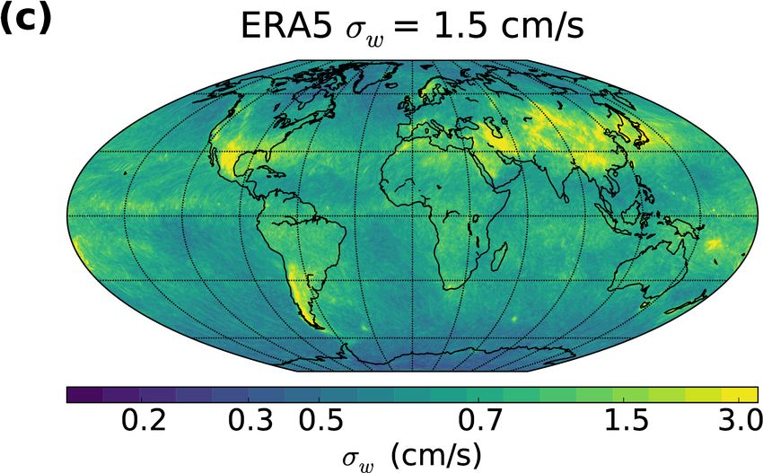
Authors Thank you, we agree. The
gures have been changed as suggested.
4. Reviewer 4. Figure 3: it is quite hard to see the relationship between the values
in right-hand panels due to the thickness of the black line and how much it jumps
around on top of the red and blue lines. I would suggest replotting it somehow so
that the reader can actually see the coloured lines - maybe make the black lines
thinner and reduce the heaviness of the gridlines to compensate visually?
Authors Thank you for the suggestion, we have adjusted Figure 3, which is more
legible now.
5. Reviewer 5. P12L31: is this speci
cally zonal momentum
ux?
Authors Yes, this is now speci
ed.
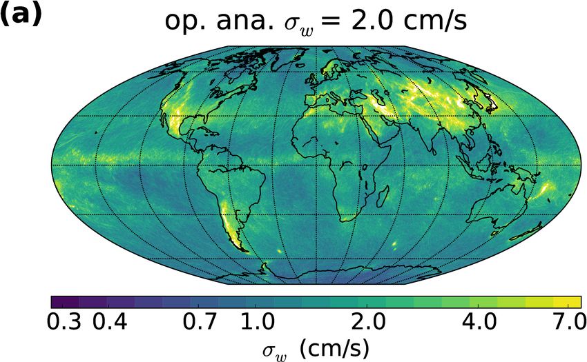
6. Reviewer Figure 5 uses a jet colour table. This is hard for colourblind readers
to read, and also suggests semantic meaning at sharp colour transitions where none
is implied by the data. I would strongly suggest changing the colour table used for
this
gure. Also, some of the maximal regions are out of band on the colour table
and plotted in white - it may be useful to truncate the data at these points to avoid
this issue.
Authors We were not aware of this, thank you for raising that point. The
colormap has been changed for Viridis.
Authors Typos and grammar mistakes have been corrected, thank you for point-
ing them out.
2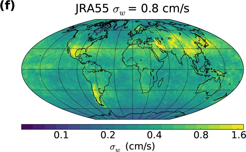
Lagrangian Gravity Wave spectra in the lower stratosphere
of current (re)analyses: reply to reviewer 2
June 9, 2020
Reply to reviewer 2
We thank reviewer 2 for their evaluation of our paper and the constructive comments.
Their suggestions for improvement have been taken into account. Please
nd below our
point by point reply.
1. Reviewer The authors use balloon data to assess the gravity wave spectrum in
various reanalyses and one operational analysis. Although they
nd that that reanal-
yses represent the shape of the spectrum well, the variability is lacking compared to
the balloons especially at higher intrinsic frequencies. Models with higher horizontal
and vertical resolution represent the gravity wave variability better, although vertical
resolution seems to have less of an eect than might be expected. They also show
that including the balloon observations in the reanalyses improves the representation
of gravity wave variance at low frequencies.
This paper is very well written and clearly organized. The results are very relevant
and of great interest to modelers. These results will help give guidance to modelers
trying to improve the representation of gravity waves in their models, both explicit
and paramereterized waves. I recommend this paper be published with a few minor
considerations below.
Authors Thank you
2. Reviewer "Furthermore, due to their expected small horizontal scale the impor-
tance of non hydrostatic eects..." Should there be an "and" in here? Otherwise this
sentence doesn't really make sense to me.
Authors Yes, thank you. This has been corrected.
3. Reviewer p.10, line 19: According to this equation, R(ω) should go to 0 as ω
approaches f, but the Figure shows R(ω) goes to in
nity as ω approaches f.
Authors Actually, there was a sign error in the
gures: the black line was depict-
ing |f | = −f (since Vorcore
ew in in the Southern hemisphere) instead of f . Thank
1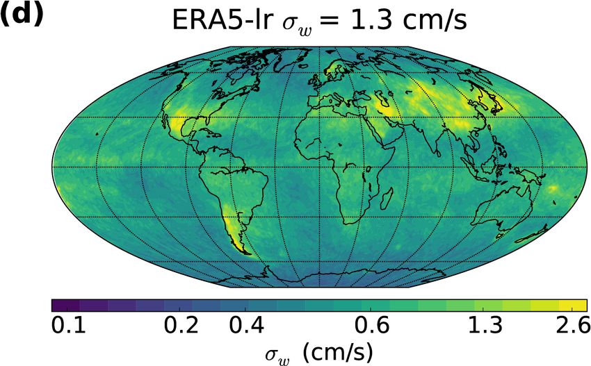
you for pointing this out, it is now corrected. We also speci
cally warn the reader
about the sign of f below the formula.
4. Reviewer p. 12, line 21: I would say "The latter behavior. . ." instead of "This
last behavior. . ."
Authors Changed as suggested.
5. Reviewer p. 15, line 29: I would say "... , it is more prevalent at the lowest
intrinsic frequencies..." also, pronounced would be a better word than prevalent.
Authors Changed as suggested.
6. Reviewer p. 15, lines 29-34: What about the in
uence of vertical resolution on
this plot? In particular it seems like there is a clear distinction between the higher
vertical resolution models and lower vertical resolution models in the u'w' columns
for both pole and tropics.
Authors Not exactly, since ERA5 has a higher vertical resolution than
ECMWF(see Table 2). This point is now mentioned in the manuscript.
7. Reviewer p. 15, line 30: This sentence doesn't really make sense grammatically:
"Indeed, while Ekh than for variables with variance primarily contained at large w." I
suggest maybe "Indeed, the dependency on horizontal resolution is more pronounced
for Ekh than for variables with variance primarily at large w."
Authors Changed as suggested
8. Reviewer p. 16, lines 6-14: What about adding the truncated ERA5 to Figure 8?
Would this provide more clues to the importance of horizontal vs vertical resolution?
Authors Comparing the degraded ERA5 to the full ERA5 only provides us with
a lower boundary for the dependence on horizontal resolution. Indeed, although it
lters out small-scale waves, the low-resolution ERA5 has the same (high-resolution)
sources of large-scale waves as the full ERA5, so that it still contains "information"
provided by the high horizontal resolution for that part of the spectrum. Because
of that, ERA5-lr shound not be considered a high vertical resolution ERA interim,
and the dierence between ERAi, ERA5-lr and ERA5 cannot be solely attributed to
either horizontal or vertical resolution. We now explain this point in more details in
the manuscript.
9. Reviewer p. 16, line 10: broken o sentence: ". . . arise from the dierent
propagation properties and ."
Authors Missing "Sources". This has been corrected.
10. Reviewer p. 25, Figure 4: The labels are quite tiny.
Authors We agree. They have been enlarged.
2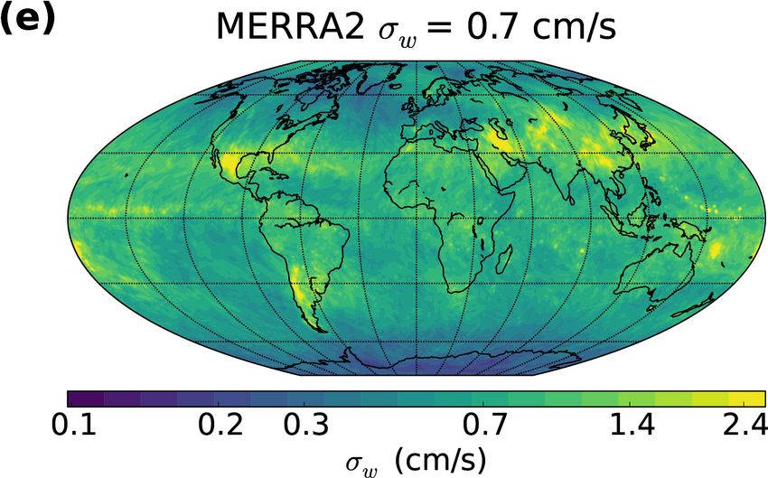
Lagrangian Gravity Wave spectra in the lower stratosphere of
     current (re)analyses
     Aurélien Podglajen1,2 , Albert Hertzog1 , Riwal Plougonven1 , and Bernard Legras1
     1
       Laboratoire de Météorologie Dynamique (LMD/IPSL), École polytechnique, Institut polytechnique de Paris, Sorbonne
     Université, École normale supérieure, PSL Research University, CNRS, Paris, France
     2
       formerly at Forschungszentrum Jülich (IEK-7: Stratosphere), Jülich, Germany
     Correspondence to: Aurélien Podglajen (aurelien.podglajen@lmd.polytechnique.fr)

     Abstract.
         Due to their increasing spatial resolution, numerical weather prediction (NWP) models and the associated analyses resolve
     a growing fraction of the gravity wave (GW) spectrum. However, it is unclear how well this “resolved” part of the spectrum
     actually compares to the actual atmospheric variability. In particular, the Lagrangian variability, relevant, e.g., to atmospheric
5    dispersion and to microphysical modeling in the Upper Troposphere-Lower Stratosphere (UTLS), has not yet been documented
     in recent products.
         To address this shortcoming, this paper presents an assessment of the GW spectrum as a function of the intrinsic (air
     parcel following) frequency in recent (re)analyses (ERA-Interim, ERA5, the ECMWF operational analysis , MERRA-2 and
     JRA-55:::
           and::::::::::
               MERRA-2). Long-duration, quasi-Lagrangian balloon observations in the equatorial and Antarctic lower strato-
10   sphere are used as a reference for the atmospheric spectrum and compared to synthetic balloon observations along trajectories
     calculated using the wind and temperature fields of the reanalyses. Overall, the reanalyses represent realistic features of the
     spectrum, notably the spectral gap between planetary and gravity waves and a peak in horizontal kinetic energy associated
     with inertial waves near the Coriolis frequency f in the polar region. In the tropics, they represent the slope of the spectrum
                              :::::::::::::::::::

     at low frequency. However, the variability is generally underestimated, even in the low-frequency portion of the spectrum. In
15   particular, the near-inertial peak, although present in the reanalyses, has a much reduced magnitude compared to balloon ob-
     servations. We compare the variability of temperature, zonal
                                                            ::::
                                                                  momentum flux and vertical wind speed, which are related to low,
     mid and high frequency waves, respectively. The distributions (PDFs) have similar shapes, but show increasing disagreement
     with increasing intrinsic frequency. Since at those altitudes they are mainly caused by gravity waves, we also compare the
     geographic distribution of vertical wind fluctuations in the different products, which emphasizes the increase of both GW vari-
20   ance and intermittency with horizontal resolution. Finally, we quantify the fraction of resolved variability and its dependency
     on model resolution for the different variables. In all (re)analyses products, a significant part of the variability is still missing
     and should hence be parameterized, in particular at high intrinsic frequency. Among the two polar balloon datasets used, one
     was broadcast on the global telecommunication system for assimilation in analyses while the other is made of independent
     observations (unassimilated in the reanalyses). Comparing the Lagrangian spectra between the two campaigns shows that they
25   are largely influenced by balloon data assimilation, which especially enhances the variance at low frequency.

                                                                      1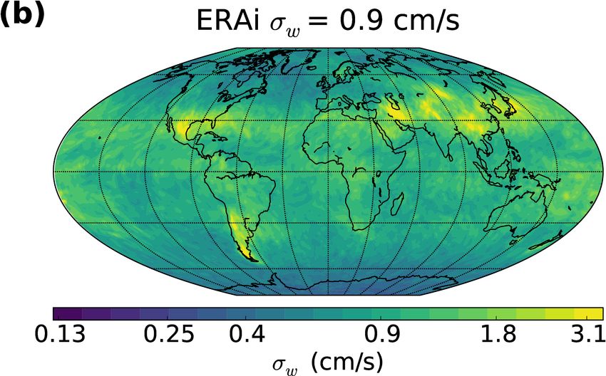
1    Introduction

     Atmospheric gravity waves (GWs) are mesoscale motions with large-scale impacts, notably through 3 mechanisms. First,
     they transport momentum from lower levels and deposit it higher up in the atmosphere, which forces large-scale circulations
     (Andrews et al., 1987), such as the Quasi-biennal oscillation (QBO, Baldwin et al., 2001). Second, they generate small-scale
5    turbulence (e.g., when breaking), which contributes to mixing atmospheric trace constituents (Podglajen et al., 2017) and dia-
     batic heating. Third, GWs induce temperature and wind fluctuations which impact the formation and microphysical properties
     of clouds (e.g., cirrus clouds, Potter and Holton, 1995) and aerosols.
         Because of those large-scale effects, GWs need to be represented in global atmospheric models. In current climate models
     with resolutions of the order of 100 km, GWs are mostly unresolved and need to be parameterized. On the contrary, global
10   weather forecast models, which currently have resolutions down to about 10 km or less, may now start to resolve a significant
     portion of the GW spectrum (e.g. Preusse et al., 2014; Jewtoukoff et al., 2015; Holt et al., 2016). However, the exact fraction
     of GWs resolved depends not only on the nominal resolution of the model, but also on the parameterized diffusion and on
     the representation of wave sources like tropospheric convection (Stephan et al., 2019). A common flaw of resolved GWs in
     models appears to be an underestimation of wave amplitude and an overestimation of horizontal wavelengths (e.g. Geller et al.,
15   2013; Holt et al., 2017). Even in models with realistic GW generation, a lack of realism in the propagation and dissipation
     of the waves often renders additional GW parameterization necessary in order to obtain a realistic general circulation (Holt
     et al., 2016, 2017). Hence, for a given model with a given resolution, it is not clear a priori what GWs are represented and
     what should be parameterized. This problem will become increasingly important as the models increase their resolution in the
     so-called ”gray zone”, resolving a larger part (but not all) the GW spectrum and its sources.
20       Crucial for climate and weather forecast models, the question of the fraction of resolved GWs is also important in (re)analyses.
     Those products have been used to investigate some properties of the GW field (e.g. Preusse et al., 2014). Reanalyses are also
     widely employed as input to trajectory calculations, notably (but not only) in the Upper Troposphere-Lower Stratosphere
     (UTLS), in order to understand, e.g., transport (e.g. Tzella and Legras, 2011), chemistry (e.g. Konopka et al., 2010) or cirrus
     cloud formation (e.g. Jensen and Pfister, 2004; Schoeberl et al., 2015; Ueyama et al., 2015). Among those three processes,
25   cloud formation (Spichtinger and Krämer, 2013; Dinh et al., 2016) is especially sensitive to mesoscale fluctuations of wind
     and temperature, so that a number of parameterizations have been developed to account for them (e.g. Bacmeister et al., 1999;
     Jensen and Pfister, 2004; Gary, 2006). A difficulty is that the parameterized fluctuations need to be similar to the perturbations
     experienced by air parcels (i.e., Lagrangian).
         Recently, Podglajen et al. (2016b) used long-duration superpressure balloon (SPB) observations to characterize Lagrangian
30   wind and temperature fluctuations due to GWs in the lower stratosphere. SPB are especially suited for gravity wave studies
     since they follow the wind and directly provide access to the intrinsic frequency ω̂ of the waves. Podglajen et al. (2016b)
     proposed a parameterization of the vertical wind and temperature fluctuations for Lagrangian trajectory models that use
     (re)analyses to compute the trajectory path. A simpler-to-implement version of the parameterization approach and its salient
     features are presented in Kärcher and Podglajen (2019). However, both Podglajen et al. (2016b) and Kärcher and Podglajen

                                                                      2
(2019), like other authors, implicitly assumed that most of the GWs seen in the observations were absent from the original
reanalysis products. In the present paper, we compare GW induced fluctuations in modern (re)analyses from the same point of
view as SPB, i.e. a Lagrangian point of view, to determine which part of the GW spectrum they resolve and how this resolved
part compares with observations. Particular focus will be spent on the intermittency of the gravity wave fluctuations in the
5 (re)analyses.
Besides the interest for studies using Lagrangian trajectories, the comparison presented here also serves another purpose, this
time from the point of view of model developers. For different models there are different criteria of success, a priori empha-
sizing the representation of the large-scale circulation. As the resolution of the models increases, a richer array of phenomena
is present in the resolved fields and the question arises whether or not to assimilate information on these processes. In that
10 respect, assessing model errors on the GW field, which is described in both observations (e.g. radiosondes, GPS temperature
profiles) and model output, is essential from the modelers’ point of view. The long-duration balloon dataset provides a unique
opportunity to perform such a task and assess the realism of modeled GW in the lower stratosphere.
The paper is organized as follows. Section 2 presents the balloon dataset and reanalyses used, as well as the comparison
methodology. Then, the results and comparisons are presented in Sect. 3 and discussed in Sect. 4. Finally, summary and
15 conclusions are provided in Sect. 5.
2 Datasets and Methodology
2.1 Long-duration balloon observations
Most observations of the atmosphere are obtained either at a fixed location (Radar, lidar) or in motion relative to the flow
(satellite, aircraft). In both cases, the relative speed between the measuring instruments and the air hampers direct Lagrangian
20 analysis of flow variability. One of the platforms which overcome that limitation are long-duration superpressure balloons
(SPB), which provide observations in a quasi-Lagrangian frame of reference (e.g. Hertzog et al., 2002; Podglajen et al., 2016a).
In the present study, we use SPB measurements as a reference to evaluate the representation of Lagrangian (quasi intrinsic-
frequency) spectra. The observations were gathered in the Lower Stratosphere (16-20 km above sea level) during three SPB
campaigns coordinated by the French Space Agency (CNES): Vorcore, PreConcordiasi and Concordiasi. Table 1 summarizes
25 the location and timing of the campaigns, as well as the sampling frequency and status regarding data assimilation. Vorcore
and Concordiasi took place in the Southern polar vortex during austral spring, while Preconcordiasi flights were launched from
an equatorial location (the Seychelles) in boreal spring. Whereas data from the later Concordiasi campaign was broadcast on
the Global Telecommunication System (GTS), the earlier Vorcore and PreConcordiasi observations are independent datasets
which can be used to evaluate reanalyses (Boccara et al., 2008; Podglajen et al., 2014). For that reason, we will focus in Sect. 3
30 on Vorcore and PreConcordiasi, while Concordiasi will be used to assess the impact of balloon data assimilation in Sect. 4.1.
During the three campaigns, a whole set of measurements was performed, including e.g. ozone and particle measurements; for
our purpose, however, only the horizontal position of the balloon from the on-board GPS, and pressure and temperature from
the Thermodynamic SENsor (TSEN) will be used.
3Table 1. Balloon measurement campaigns used as observational reference for this study. The last column (data assimilation) reports whether
or not the data was broadcast on the Global Telecommunication System.
Balloon geographic altitude number period measurement measurement data
campaign location (density) of balloons sampling precision assimilation
launched [evtl. accuracy]
Vorcore Southern 16-20 km 25 Sep. 2005 to u, v: 15 min u, v: < 0.05 m s−1 No
3
polar vortex (0.08-0.13 kg/m ) Jan. 2006 p: 1 min p: 1 Pa
Concordiasi Southern 16.5-18 km 19 Sep. 2010 to u, v: 1 min u, v: 0.025 m s−1 Yes
3
polar vortex (0.10-0.12 kg/m ) Jan. 2011 p: 30 s p: 1 Pa
PreConcordiasi Tropics and 19-20 km 3 Feb. 2010 to u, v: 1 min u, v: 0.025 m s−1 No
3
southern mid-latitudes (0.10-0.12 kg/m ) May 2010 p: 30 s p: 1 Pa
Apart from occasional changes in the mass or volume of the system (such as dropsonde launching, changes in the incoming
radiation flux) and balloon inertia acting at periods shorter than 15 min (Vincent and Hertzog, 2014; Podglajen et al., 2016b),
SPB are essentially passively advected on isopycnic (constant-density) surfaces once they have ascended to their equilibrium
level in the stratosphere. This quasi-Lagrangian behavior renders measurement interpretation relatively simple. Horizontal
5 winds u and v are deduced from the successive positions of the balloon, while pressure is directly measured by the TSEN
meteorological sensors. In case of slightly uneven time sampling (varying sampling time step), the raw measurements were
interpolated linearly onto a regular time grid. A fast Fourier transform algorithm was then applied to the time series, yielding
the signal’s Fourier transform (û(ω̂), v̂(ω̂), p̂(ω̂)). Periodograms are then obtained directly from |û(ω̂)|2 , |v̂(ω̂)|2 and |p̂(ω̂)|2 .
In practice, we use a variant of Welch’s method and estimate spectra by averaging periodograms obtained from 8-day windows
10 with 4 days overlaps. Note that for consistency with, e.g., Fritts and Alexander (2003), our definition of the intrinsic-frequency
Fourier transform is such that the inverse transform reads:
+∞
Z
(u(t), v(t), p(t)) = (û(ω̂), v̂(ω̂), p̂(ω̂))e−i ω̂ t dω̂ (1)
−∞
While this sign convention does not affect the periodograms (estimated from squared modulus quantities and insensitive to
the phase), it matters as far as the phase of the signal is concerned, notably for the polarization relations relating the Fourier
15 transforms of the different variables.
Combining the spectra of |û|2 (ω̂) and |v̂|2 (ω̂) leads to the horizontal kinetic energy spectrum Ekh (ω̂) per unit mass:
1 2
|û| (ω̂) + |v̂|2 (ω̂)
Ekh (ω̂) = (2)
2
On the other hand, pressure fluctuations p0 along the balloon trajectory can be used to estimate the vertical displacement of
isopycnic surfaces ζρ0 and isentropic surfaces ζθ0 along air-parcel trajectories (see Hertzog et al., 2002; Podglajen et al., 2014,
20 2017):
1 0 1 0
ζθ0 = ζρ = − p (3)
α g ρ̄α
4 .
g g
where ρ is the average segment density, α = Cp + ddzT̄ R + ddzT̄ depends on the local temperature lapse rate dT̄ /dz (g
is the gravitational acceleration, Cp the thermal capacity of air at constant pressure and R the gas constant for air). dT̄ /dz is
dT̄
not directly measured but interpolated from the ECMWF ERA5 reanalysis; the sensitivity to the exact value of dz is small
and does not affect the conclusions presented below. Relation 3 relies on a few assumptions (small vertical excursions, small
5 Eulerian pressure perturbation relative to temperature perturbations, adiabatic and hydrostatic flow) which are well-met for
the intermediate-frequency (periods between 1 day and 15 minutes) motions of interest here (as they are the ones resolvable
by the reanalyses). Using Eq. 3, the potential energy spectrum per unit mass Ep can be deduced from the estimated pressure
spectrum:
1 1 N2
Ep (ω̂) = N 2 |ζθ0 |2 = |p̂|2 (ω̂) (4)
2 2 (g ρ̄α)2
10 As an illustration, Figure 1 (updated from Podglajen et al. (2016a)) shows the intrinsic-frequency spectra (power spectral
densities) of Ekh , Ep and of the zonal momentum flux per unit mass u0 w0 for the Concordiasi (polar) and PreConcordiasi
(tropical) campaigns, which have the highest sampling frequency (Table 1). The important characteristics that are present in
the observations and will be searched for in the reanalyses are:
– in the polar region, a spectral gap at f between low frequencies and GW frequencies, seen in both Ep and Ekh . Then,
15 a local peak in Ekh at frequencies just higher than f , almost absent in Ep . In that frequency range (f < ω̂ < 4 f ),
Ep < Ekh .
– in the tropics and in the mid-frequency range (ω̂
f ) for the polar latitudes, the spectra scale with a power-law behavior
ω̂ −s with s ' 2 for Ep and Ekh , and s ' 1 for |u0 w0 |. This scaling appears until ω̂ ' 100 cy/day.
Above about 100 cy/day, the balloon-observed Ep and |u0 w0 | increase and peak near the Brunt-Väisälä frequency N . Al-
20 though there exist potential physical reasons for a spectral peak of momentum and potential energy near N in the atmosphere
(Podglajen et al., 2016a), part of the balloon-observed enhancement is likely an artifact caused by the non-isopynic response
of the platform (Podglajen et al., 2016a; Vincent and Hertzog, 2014). Furthermore, due to their expected small horizontal scale
and
:::
the importance of non hydrostatic effects (absent from hydrostatic weather models), we can safely assume that buoyancy
waves (near N ) are absent from hydrostatic, low resolution analysis weather forecast models. Hence, we will focus our analysis
25 to ::
on:intrinsic frequencies smaller than 48 cy/day (periods larger than 30 min). For pressure observations, there is a significant
aliasing at 48 cy/day from higher-frequency motions (in particular near the N -peak); this is overcome by averaging pressure
observations at the highest-available frequency (1 min for Vorcore, 30 s for Concordiasi and PreConcordiasi, see Table 1) with a
15-minute Hann window weighting function and using this subsampled, low-pass-filtered version of the data in the subsequent
analysis.
30 2.2 Atmospheric (re)analyses
For this study, we ::::::
initially:considered 4 recent reanalysis systems (ERA-Interim, ERA5, MERRA-2 and JRA55:::::::
JRA-55) and
the ECMWF operational analysis (corresponding to the model versions used in February and December 2010, i.e. at the times
5pole tropics
102 Ep 102 Ep
u0w0 u0w0
Ekh Ekh
100 100
-1.8 -2.1
m2 s−2 /(cycle/day)
m2 s−2 /(cycle/day)
10 −2 ωb 10 −2 ωb
10−4 10−4
10−6 f N 10−6 N
10−8 1 10.0 100.0 10−8 1 10.0 100.0
Intrinsic frequency (cycle/day) Intrinsic frequency (cycle/day)
Figure 1. Average spectra of horizontal kinetic energy Ekh , potential energy Ep and |u0 w0 | inferred from SPB observations during the (left)
polar and (right) equatorial balloon campaigns in 2010.
of the PreConcordiasi and Concordiasi balloon campaigns). The model version and spatial resolution of the different products
are summarized in Table 2, together with the time resolution at which the outputs (reanalyses and forecasts) are saved and/or
made available. For more details regarding the model set-ups, physical parameterization and data assimilation flow, we refer
the reader to the S-RIP introduction paper (Fujiwara et al., 2017).
5 Due to finite storage ability, the (output) time sampling is rather coarse (hourly at the best). This may have been a limiting
factor for our study: GWs indeed have intrinsic periods ranging from 12 hours down to a few minutes (see Fig. 1), so that with
fields output every 3 or 6 hours the dominant fraction of GW variance is aliased towards lower frequencies, thus potentially
affecting our estimates. However, this limitation is mitigated by the fact that we analyse spectra as a function of intrinsic
frequency ω̂:
10 ω̂ = ω − kū − lv̄ (5)
which
::::::
combines the ground-based frequency of the motion ω and its horizontal scale (given by the zonal and meridional
wavenumbers k and l). Investigations of different time sampling with ERA5 (for which hourly outputs are available) demon-
strated that, while in polar regions the considered intrinsic frequency spectra are strongly sensitive to a change of time sampling
from 6 to 3 hours, even more frequent (than 3-hourly) sampling only marginally affected the results. In light of this, the main
15 body of the paper will not present the results obtained with JRA55JRA-55,
::::::
available only every 6 hours (see Table 2) for which
our :::::::
spectral analysis suffers from aliasing. For a fair comparison, all (re)analyses (including ERA5) will be used at a time
resolution of 3 hours, except in Appendix A where the impact of the output frequency is investigated.
6Table 2. Description of the resolution of the models/(re)analyses used in this study. For the spectral models, N corresponds to the reduced
Gaussian grid, F to the full Gaussian grid, and an approximate resolution is given. For the horizontal grid, cs: cubed sphere; sp: spectral
model. Further information on the reanalysis systems can be found in Fujiwara et al. (2017).
(Re)analysis center operational horizontal Horizontal retrieved number of levels time between available Reference
model version grid type grid spacing horizontal between successive time resolution
resolution 16 and 20 km analyses (hours) incl. forecasts (hours)
MERRA-2 NASA GEOS 5.12.4 (2015) CS 1/2◦ lat× 1/3◦ lon native 4 3 Bosilovich et al. (2015)
∼ 60 km
JRA-55 JMA JMA GSM (2009) sp N160∼ 55 km F160 3 6 6 Kobayashi et al. (2015)
ERA-Interim ECMWF IFS Cy31r2 (2007) sp N128∼ 79 km (1◦ )2 4 6 3 Dee et al. (2011)
ERA5 ECMWF IFS Cy41r2 (2016) sp N320∼ 31 km (0.3◦ )2 12 1 1 Hersbach et al. (2019)
op. ECMWF ECMWF IFS Cy36r1 (2010) sp N640∼ 16 km (1/8◦ )2 8 6 3
2.3 Comparison methodology
A simplistic approach to compare balloon observations and reanalyses would be to interpolate the model fields along the
actual balloon trajectory. However, this might lead to erroneous conclusions regarding the variability present: if for instance
the balloon were to record a vertical oscillation with a sheared flow u in the reanalysis, this may lead to an oscillation in the
5 interpolated u wind although they would :::::
might :be absent from an actual trajectory computed with the reanalysis wind. To
avoid that complication, we directly computed isopycnic (balloon-like) trajectories using the reanalysis fields. In other words,
we solve the following system of ordinary differential equations:
dX = u(X, Y, Z, t)
dt
dY (6)
dt = v(X, Y, Z, t)
Z = ζρ (X, Y, Z, t)
the air density ρ being a strictly decreasing function of geometric altitude. In practice, System 6 is solved with ln(ρ) as the
10 vertical coordinate, and the 2D trajectories are integrated using a Runge-Kutta scheme of order 4 and a time step of 1 minute,
adjusted when needed to satisfy the CFL criterion. We note that the dependency of the trajectory on the integration time step
and the details of the numerical scheme is small compared to other sources of errors (Bowman et al., 2013). Gridded reanalyses
fields (typically p, T , u and v) are interpolated in the horizontal and time dimension using cubic splines, leading to vertical
profiles; then the vertical coordinate ln(ρ) is calculated and finally the wind is interpolated at the density level of the balloon. To
15 examine the Lagrangian variability and estimate spectra, we calculate 8-days trajectories started at the balloon position every
4 days, thus matching the segments used in the observations. Examples of such trajectories for ERA5 reanalysis are displayed
in Fig. 2.
At this point, two remarks should be made. First, regarding trajectory accuracy: while it is affected by the sampling frequency
(in space and time) of the model and the interpolation method used (Stohl et al., 1995; Bowman et al., 2013), the main source
20 of uncertainty in the lower stratosphere stems from errors in the reanalysis fields (Boccara et al., 2008; Podglajen et al., 2014).
7In polar regions, the analyses compare well to observations at lower stratospheric altitudes (Boccara et al., 2008), so that there
is generally not much difference between observed and simulated balloon trajectories over periods of ∼8 days, as illustrated
in Fig. 2 for the case of ERA5. In the tropics, on the contrary, analyses may exhibit large deficiencies (Podglajen et al., 2014;
Dharmalingam et al., 2019), and the computed trajectories can largely diverge from the observed ones. However, our results are
5 not overly sensitive to the exact number and location of trajectory segments used. Errors in the large-scale wind are deemed very
unlikely to generate a sampling bias and artificially degrade GW variability (which they could do in particular and improbable
cases, e.g., by making the balloons drift systematically in quieter areas than those where they actually flew).
30°W 0° 30°E
52
60°W 60°E 54
b2
b2
56
pressure (hPa)
90°W 90°E
58
isopycnic isopycnic 60
120°W isentrope 120°E isentrope
3D kinematic 3D kinematic
3D diabatic 3D diabatic 62
balloon isentropic estimated from isopycnic
balloon
150°W 180° 150°E
306 307 308 309 310 311 312
day of year
Figure 2. (Left) Observed and calculated horizontal trajectories of Vorcore Balloon 2 started from its position on 2005/11/02 at 00:00 UTC.
The calculated trajectories are 3D-kinematic (with omega velocity, black), 3D-diabatic (with diabatic heating rates, orange), 2D-isentropic
(blue) and 2D-isopycnic (red) trajectories; all were computed using ERA5 wind and temperature field at 3-hourly output resolution. The
observed trajectory of the balloon is shown in grey. (Right) Pressure time series corresponding to the horizontal trajectories on the left panel.
Please note that the y-scale only covers a narrow range of altitudes (roughly 1 km maximum deviation peak-to-peak, i.e. about 3 model levels
:::::::::::::::::::::::::::::::::::::::::::::::::::::::::::::::::::::::::::::::::::::::::::::::::::::
for ERA5).
:::::::::
Second, we note that physical applications and process studies are interested in air parcel trajectories, which are a priori
distinct from the isopycnic trajectories of the balloons. However, as argued above and in Podglajen et al. (2016b), the horizon-
10 tal positions of isopycnic, isentropic and true air parcel trajectories should remain close (relative to the distance traveled) at
synoptic time scales (a few days), and Equation 4 is expected to be a good approximation in the stratosphere with low diabatic
heating. In order to verify this, we compared the 8-day trajectories and spectra for isopycnic, isentropic (constant potential
8temperature θ) and full-3D trajectories, computed either in p coordinate with ω = Dp/Dt as vertical velocity (kinematic tra-
jectories) or with θ coordinate and θ̇ vertical velocity (diabatic trajectories). The different horizontal and vertical trajectories
for the special case of Vorcore balloon 2 on 2005/11/02 are displayed on Fig. 2.
Figure 2 demonstrates the validity of our approximations for ERA5: the 3 trajectory types only slightly diverge from one
5 another in the horizontal. Although as expected the isopycnic trajectory diverges more rapidly from the 3D trajectory than the
isentropic one, for an integration time of 8 days the paths remain close. While their vertical positions are clearly distinct, the
isentropic, 3D-kinematic and isopycnic (scaled onto the isentropes using Eq. 3) trajectories are highly correlated at short time
scales. As examined in Appendix B, the estimated Lagrangian energy spectra exhibit only slight differences. Hence, for a more
direct comparison to balloon observations, we considered isopycnic trajectories (adjusted using Eq. 3) in the following.
10 3 Results: Intrinsic frequency spectra of Lagrangian fluctuations
In Fig. 3 are depicted the intrinsic frequency spectra (power spectral density or PSD) of Ekh , Ep and the zonal pseudo-
momentum flux (1 − f 2 /ω̂ 2 )|u0 w0 | = (1 − f 2 /ω̂ 2 )< (ûŵ∗ ) (1 − f 2 /ω̂ 2 )|u0 w0 | = (1 − f 2 /ω̂ 2 ) |< (ûŵ∗ )| derived from isopyc-
::::::::::::::::::::::::::::::::::::
nic trajectories computed using 3-hourly wind data from the different (re)analyses. The trajectories are output every 15 min-
utes, so that from the point of view of the sampling, the highest resolvable frequency (Nyquist frequency) in the spectra is
15 1/48 cy/day. However, we should recall that, as mentioned above and explained in Appendix A, the effective resolution in
terms of intrinsic frequency actually depends the limited time and the space resolution of the (re)analyses.
3.1 Horizontal kinetic energy spectra Ekh (ω̂)
The top two panels of Fig. 3 show the Ekh spectra (solid lines) obtained from polar (Vorcore, left) and equatorial (PreConcor-
diasi, right) trajectories for the balloon observations (black lines) and the reanalyses (colors). In the polar case, low frequency
20 features (below the Coriolis frequency f ) are well-represented all reanalyses. However, in the gravity wave frequency-range
(above f ), the variance in Ekh is largely underestimated in all 3 systems compared to observations. Nevertheless, the reanalysis
Ekh -spectra exhibit typical features similar to the observations, including:
1. a local minimum in Ekh between f /2 and f , the characteristic spectral gap separating GW (ω̂ > f ) from synoptic-scale
motions (ω̂ < f )
25 2. a local maximum in Ekh around 1.2 − 1.5 f (the near inertial peak, see Hertzog et al. (2002))
3. a power-law decrease in Ekh for frequencies larger than 1.5 f
The differences between reanalyses and observations mainly concern:
1. the frequency at which the peak around f in Ekh (ω̂) occurs and its magnitude.
2. the power-law slope of the decreasing Ekh for ω̂
f . The observations have the shallower slope, followed by ERA5
30 and ERA-Interim, MERRA-2 having the steepest slope.
9Despite the quantitative disagreement between the different reanalyses, they also exhibit qualitative similarities with one
another and with the observations. In particular, they all show a near-inertial Ekh -peak, consistent with observations (Hertzog
et al., 2002).
In order to further investigate the agreement between the resolved perturbations and gravity wave theory, we examine to
5 what extent the polarisation relation for inertio gravity waves are fulfilled. On the f -plane, with the convention given by Eq. 1,
the polarization relation for the horizontal wind reads (Fritts and Alexander, 2003):
ω̂
ûk (ω̂) = i û⊥ (ω̂) (7)
f
where ûk is the amplitude of the horizontal wind along the wave vector and û⊥ the amplitude perpendicular to the wave
vector. Keeping in mind the convention expressed by Eq. 1, Equation 7 indicates that low-frequency waves (near f ) induce
10 anticyclonic flow rotation whereas high frequency waves have their horizontal wind perturbation aligned with the wave vector
and no preferred rotation direction. To make use of this property and further demonstrate that the near-inertial peak in the
analyses is due to inertial oscillations, we turn to rotary spectral analysis. The rotary Fourier transform of the horizontal wind,
Û , is defined by:
Û (ω̂) = û(ω̂) + iv̂(ω̂) (8)
15 As a consequence of Eq. 7, the rotary ratio R(ω̂), ratio of the PSD of anticlockwise horizontal motions (|Û (−ω̂)|2 with our
Fourier transform convention in Eq. 1) and clockwise ones (|Û (ω̂)|2 ), verifies the relation:
2 !2
Û (−ω̂) 1 − ω̂f
R(ω̂) ≡ = (9)
Û (ω̂) 1 + ω̂f
Note that the rotary ratio depends on the sign of f , so that the rotation direction is reversed in the southern hemisphere with
:::::::::::::::::::::::::::::::::::::::::::::::::::::::::::::::::::::::::::::::::::::::::::::::::::::
respect to the northern hemisphere, with anticyclonic motions being always favored.
::::::::::::::::::::::::::::::::::::::::::::::::::::::::::::::::::::
20 Equation 9 has been exploited in previous studies (e.g. Hertzog et al., 2002; Conway et al., 2019) to evaluate the consistency
of the observed horizontal wind spectrum with linear gravity wave theory. In particular, the dominance of anticyclonic (here
in the Southern hemisphere) motions at low frequencies is consistent with Eq. 9 and indicates the importance of linear gravity
waves, opposed to, e.g. stratified turbulence for which no systematic phase relation between the horizontal wind components
is expected. In Fig. 3, R(ω̂) is displayed together with its theoretical value ratio given by Eq. 9. The dominance of anticyclonic
25 motions is a further argument in favor of inertio-GW being responsible for the f -peak in both reanalyses and observations.
However, we note that it is less pronounced in the reanalyses than in the observations, and in ERA5 than ERA-Interim and
MERRA-2. Possible reasons for this will be examined in the next section.
In the tropics, the statistical agreement between reanalyses and observations regarding the representation of high-frequency
variability is surprisingly better than in the polar latitudes. This contrasts with the representation of large-scale wind field which
30 is better in polar regions (Boccara et al., 2008) than in equatorial ones (Podglajen et al., 2014). The agreement obtained for low-
frequency waves is quantitative as well as qualitative, and reaches up to a cut-off frequency which is about 4 cycles/day for the
10ERA-Interim, ERA5 and the ECMWF operational analysis, and 2 cycles/day for MERRA-2. Below this cut-off frequency, the
observed and modeled age spectra are in quantitative as well as qualitative agreement. At the cut-off frequency, the reanalysis
spectra show a kink and above it they drop with much larger slopes than the observed ones, which keep decaying with a
constant slope.
5 3.2 Potential energy spectra
The middle two panels of Fig. 3 show the spectra of the potential energy per unit mass Ep , for the polar (left) and tropical (right)
flights. To a large extent, the situation is similar to the one described above for Ekh : in the polar case, there is a qualitative
agreement in the structure of the power spectra (notably regarding the spectral gap around f ), but a quantitative disagreement
and a steeper power law-slope than in the observations.
10 Besides the direct value of the potential energy, it is again interesting to investigate whether the fluctuations in reanalyses
verify the polarisation relation expected for gravity waves. In the absence of constructive interference, the ratio of potential to
horizontal kinetic energy for frequencies ω̂
N should obey (Podglajen et al., 2016b):
Ekh (ω̂) ω̂ 2 + f 2
= 2 (10)
Ep (ω̂) ω̂ − f 2
Ekh (ω̂)
Figure 3 exhibits Ep (ω̂) for the 3 reanalyses and the observations (dashed lines), together with its theoretical value given
15 in Eq. 10. The observations again closely follow theoretical expectations from ∼ 1.2 f , with a dominance of kinetic energy, to
higher frequencies (the so-called mid-frequency range) where there is an equipartition between Ep and Ekh . The variability
in reanalysis trajectories shows the same evolution with frequency as the observations, and the Ekh /Ep ratio decreasing with
increasing frequency. However, reanalysis also suffer from a significant overestimation of the kinetic energy compared to the
potential energy. This is the case by a factor 1.5 to 3 for ERA5, and 5 for the ERA-Interim and MERRA-2. Together with
20 the rotary ratio analysis, this suggests that a significant fraction of the variability does not obey the observed (and expected)
polarisation relations for gravity waves. ::::
One :::::
might ::::::::
speculate :::
that::::
this :::::::::::
inconsistency :::::
stems::::
from:::::::::
numerical :::::::::
dissipation.:
In the tropics, as for the Ekh spectra, the Ep spectra from reanalyses and observations are in better agreement than over the
pole. In particular, the Ekh /Ep ratio is close to 1 for the reanalyses, as expected, whereas there is a quantitative agreement
between observed and analyzed Ep up to a threshold frequency similar to that encountered with Ekh . Beside the reanalyses,
25 for the tropical case the ECMWF operational analysis trajectories are also displayed, which shows similar quantitative results
as for the ERA5 reanalysis.
3.3 EP flux and vertical wind spectra
The bottom two panels of Fig. 3 display the zonal pseudo-momentum 1 − f 2 /ω̂ 2 |u0 w0 | flux spectra of resolved waves in
the reanalyses. This quantity characterizes the forcing of the large-scale flow by the waves so that those panels enlighten us
30 regarding the missing gravity wave drag from resolved waves compared to observations.
11Over the pole, the reanalyses underestimate the variability in the whole GW range, with ERA5 being the closest to the
balloon observations. Although the number of reanalysis products is limited, there appears to be a correlation between the
fraction of variability resolved at low frequency and the vertical resolution of the product (given in Table 2). With the highest
vertical resolution, ERA5 resolved the largest fraction of the variability, followed by ERA-Interim and MERRA-2 with coarser
5 resolutions.
In the equatorial region, on the other hand, similar to the Ekh and Ep spectra, the momentum flux by low-frequency equato-
rial GW is comparable to observations in all products, up to the threshold frequency where it drops with a slope twice as large
as the actual slope.
We do not show the vertical wind spectrum, but its shape can be readily deduced from the potential energy spectrum as Ekv =
1 2 ω̂ 2
10 ∝ N
2 ŵ Ep , so that the inequal performance of the reanalysis can be deduced from the middle panel of Fig. 3. It should
be noticed that the different quantities considered have changing power-law slopes in the gravity wave range from ω̂ −2 for the
horizontal kinetic energy Ekh and potential energy Ep power spectra, to ω̂ −1 for the EP flux spectrum 1 − f 2 /ω̂ 2 |u0 w0 |,
and to ω̂ ∼0 for the vertical kinetic energy Ekv . As a consequence, the variability of different fields emphasizes different parts
of the spectrum: while u, v (Ekh ) and T (Ep ) are more connected to the low-frequency part of the gravity wave spectrum,
1 − f 2 /ω̂ 2 |u0 w0 | corresponds to the intermediate frequencies, and the vertical wind component w (related to Ekv ) to the
15
high-frequency waves.
3.4 Intermittency and distribution of the fluctuations
The PSDs examined above inform::::::
provide::::::::::
information:on the autocorrelation and the repartition of the fluctuations as a function
of intrinsic frequency. However, as pointed out by several authors (e.g. Hertzog et al., 2012; Podglajen et al., 2016b), the
20 probability distributions are also relevant to determine whether the variance is due to ubiquitous, constant variability generated
by the superposition of random waves, or if rare, large excursions created by specific wave events can occur. This last :::
The:::::
latter
behavior is expected for GW which are known to be intermittent.
3.4.1 Intermittency of the fluctuations
Similar to what was used for the Lagrangian spectra, we compare the distribution of the fluctuations in the reanalyses to the
25 observations based on computed isopycnic trajectories corrected for the non-isopycnic behavior (by using the coefficient α de-
fined in Eq. 3). In order to focus on the GW range, we filter the outputs of the trajectories to keep only the signal corresponding
to intrinsic frequencies shorter than 48 cycles/day and larger than f (30◦ )/(2π) ' 1 cycle/day (tropics) or f (70◦ )/(2π) ' 2
cycles/day (pole). The lower bound is considered as the lower bound of the GW frequency range in the regions studied, while
the upper bound corresponds to the Nyquist frequency of Vorcore balloon position information (every 15 minutes). It is below
30 the frequency at which the balloons start to depart significantly from the isopycnic behavior, so that the comparison can only
f N
be marginally affected by the non-isopycnic balloon response. In that frequency range [f /(2π); ∼ (N/2)/(2π)][::::::::
2π ; ∼ 4π ], we
consider temperature, ::::
zonal: momentum flux and vertical velocity to characterize statistics and intermittency of respectively
low, medium and high-frequency waves.
12Figure 4 shows the probability distribution (PDF) of the three quantities (temperature, zonal
:::::
momentum flux and vertical
wind) for all the (re)analyses considered. From top to bottom, the considered fluctuations are primarily induced by waves
of increasing frequency; |Tl0 |2 ∝ Ep (ω̂) emphasizes the low frequencies while |u0 w0 | ∝ ω̂Ep (ω̂) and |w0 |2 ∝ ω̂ 2 Ep (ω̂) are
related to increasing frequencies. Since high frequency waves are more poorly represented than low frequency ones (Fig. 3), it
5 comes with no surprise that the PDF of analyzed and observed fluctuations are in increasing disagreement from temperature to
momentum flux and from momentum flux to vertical velocity in both tropical and Southern polar regions.
The width of the temperature PDFs for the polar and tropical regions is redundant with the level of the variance in the Ep
spectrum already shown in Fig. 3. The additional information provided in Fig. 4 concerns the shape of the PDF. In the tropics,
GW temperature fluctuations are ubiquitous and characterized by a Gaussian PDF. This behavior is fairly well reproduced in
10 all reanalyses examined here. In contrast, in the pole, the balloon PDFs are no longer Gaussian. In particular, they have longer
tails than Gaussian PDFs, a behavior which is reproduced by reanalyses.
Regarding the momentum flux, the tropical and polar PDFs both exhibit log normal PDFs, as well as the reanalyses. We note
that the tropical regions during PreConcordiasi show more activity than the polar regions during Vorcore, but this is largely due
to a wider GW range in the tropics, where f → 0. Finally, the vertical wind PDFs show Laplace distributions in both cases,
15 and the order of the reanalyses is the same as for the rest. In summary, while the fraction of resolved variance varies from
one analysis to the other, it appears that the basic intermittency properties of the GW field and the shape of the PDF of the
fluctuations are consistent between observations and the different reanalyses.
It should also be noticed that the conclusion regarding the resolved fraction of variability for the different reanalyses are
transferable from one campaign to the other. In other terms, for all quantities and regions examined here, we find that the more
20 realistic reanalysis is ERA5 followed by ERA-Interim and MERRA-2. The 2010 ECMWF operational model performs better
than ERA5, likely because of its superior horizontal resolution.
3.4.2 Geographic distribution of the fluctuations
We have considered above the intermittency of GWs sampled by the balloons along their trajectories. This intermittency stems
from both space and time variability of the GW field in which the balloons drift. A significant part of it comes from the
25 geographic variability of wave sources, as illustrated in Fig. 5 through global maps of the vertical wind standard deviation at
100 hPa (related to high frequency wave activity) for the month of March 2010. The geographic structure is similar between
the different reanalyses, which is consistent with the fact that intermittency is similar in the different products (see the shapes
in Fig. 4). GW amplitudes largely differ from one product to the other, but the geographic variability is to a large extent
common to all reanalyses. In the season examined (boreal spring 2010), mountain ranges such as the Rockies, the Andes,
30 the Himalaya or the Antarctic peninsula stand out as regions of large activities. Convective regions such as the Intertropical
Convergence Zone are also characterized by a larger activity in all products. However, although the general geographic pattern
of σw do match between the different products, there are differences in the details. In particular, the features are sharper and
smaller scale (especially around orography) in the high resolution products (the operational analysis and ERA5) than in the
13lower resolution reanalyses ::::::::::::
(ERA-Interim,:::::::::
MERRA-2::::
and :::::::
JRA-55). Although this property might be expected, it implies that
intermittency is increased in those products.
Since the different resolutions in the reanalyses imply different horizontal wave numbers which may undergo different
filtering and vertical propagation, we present a vertical profile of σw in the tropics for the different products in Fig. 6, panel
5 a). There is a drastic reduction in σw from the troposphere to the stratosphere, related to the increased stratospheric stability
hampering vertical motions there. Fig. 6, panel b) displays the same σw equatorial profile but normalized by the standard
deviation from the ECMWF analysis. Although they do not resolve the same wave population, the different analyses essentially
show similar vertical structure in GW variance, except ERA5 for which σw is relatively reduced around the tropopause. This is
likely due to the increased stability in that region in the high vertical resolution ERA5:, :::::
which::::
can better resolve strong vertical
:::::::::::::::::::::::
10 gradients near the tropopause.
:::::::::::::::::::::::
4 Discussion
4.1 Impact of balloon data assimilation
Balloon observations from the PreConcordiasi and Vorcore campaigns were not assimilated in the reanalyses, so that they
provide an independent evaluation of the resolved GW variability. However, data collected during the Concordiasi campaign,
15 which took place in austral winter 2010, was broadcast on the GTS and assimilated in most analyses, including ECMWF
operational data, ERA5 and ERA-Interim, and MERRA-2 (Hoffmann et al., 2017). Hence, comparing the period of the (as-
similated) Concordiasi campaign with that of the (unassimilated) Vorcore provides an opportunity to characterize the extent to
which balloon data assimilation in the atmospheric models impacts the representation of the wave field (either through spurious
wave generation or realistic waves introduced in the initial state that propagate in the forecast). Since the Concordiasi dataset
20 was only present one yearConcordiasi only flew in austral spring 2010, GW activity in the 2010 southern lower stratospheric
::::::::::::::::::::::::::::::::::::
polar vortex is not typical but largely influenced by data assimilation. However, with the development of the Loon dataset of
superpressure balloons (Conway et al., 2019) and studies regarding its assimilation in NWP models (Coy et al., 2019), it is
interesting to document the impact of such a SPB dataset.
The Ekh spectra for the two campaigns are shown in Fig. 7. There are slight differences between the two observed spectra
25 (black lines), notably with a more pronounced f -peak during Vorcore than Concordiasi. Those are likely due to the different
latitudinal sampling during the two campaigns, with more variable f for Vorcore trajectories than Concordiasi’s (see the shaded
grey area in Fig. 7). However, the main differences between the two campaigns does not lie in the observed spectra but rather
in the analyzed ones. Whereas the reanalysis Ekh spectra during Vorcore largely underestimate Ekh and in particular the
magnitude of the spectral peak near f , there is a clearer spectral peak in the reanalyses with assimilated balloon data. This
30 better performance of the reanalyses during Concordiasi shows that besides adjusting the state of the flow, assimilation of the
balloon dataset statistically reinforces some dynamical ingredients in the simulation (here inertial waves).
144.2 Impact of underlying model version and resolution on GW representation
4.2.1 Time sampling
Proper representation of the GW variability requires sufficient time resolution, in particular to avoid aliasing of the spectral
gap and the f -peak. As mentioned above, this is not as much of a critical issue for the model time step (which is small enough
5 not to filter out the GW spatially resolved) as for its time sampling. The time sampling of the reanalysis should indeed be high
enough to isolate unequivocally the highest ground-based frequency present in the simulation. Furthermore, this parameter
is one of the most sensitive in trajectory calculations (e.g. Pisso et al., 2010; Bowman et al., 2013), at least with the spatial
resolution and integration time step we used. This is especially the case since the winds are instantaneous fields rather than time
averages, which implies aliasing when subsampling (e.g. Stohl et al., 1995; Bowman et al., 2013). In order to test the impact
10 of this key parameter on our Lagrangian spectrum estimation, we performed trajectory calculations with ERA5 varying the
time sampling of the reanalysis outputs between 6, 3 and 1 hour. We use the instantaneous ERA5 wind values and do not apply
any time averaging which would reduce aliasing but cannot be applied to products with coarser temporal sampling (Hoffmann
et al., 2019).
The results of this experiment are presented in Appendix A and can be summarized as follows. First, improving the time
15 sampling of the reanalysis from every 6 to every 3 hours induces large changes in the Lagrangian GW spectrum over the pole
and enables inertial oscillations at periods of ∼ 12 hours to be resolved. On the contrary, a further improvement of the time
resolution from every 3 hours to every 1 hour has little noticeable effect, suggesting that a large fraction of the resolved high-
intrinsic frequency GW activity is actually caused by the background wind moving the air parcels across "quasi-stationary"
wave features with ground-based periods larger than about 6 hours.
20 4.2.2 Impact of vertical and horizontal resolution
The nominal resolution of the model, given in Table 2, largely controls the magnitude of GW fluctuations in reanalyses. This is
shown in Figure 8, which displays the fraction of resolved variance in the 2-48 cy/day intrinsic frequency range in the reanalysis
products compared to balloon observations, for the horizontal kinetic energy Ekh , the potential energy Ep , the zonal pseudo-
momentum flux 1 − f 2 /ω̂ 2 |u0 w0 | and the vertical kinetic energy Ekv . Considering the (re)analyses from ECMWF (i.e.
25 ERA-Interim, ERA5 and op. ECMWF), the sorting of the resolved variance reflects the horizontal resolution of the products,
for all considered variables. MERRA-2 stands out in this consideration: although its nominal resolution(∼ 60 km, see Table 2)
is better than that of ERA-Interim (∼ 79 km),::
it::::::::::::
systematically:::::::
resolves::a :::::::
smaller ::::::
fraction:::
of ::::
GW :::::::
variance. However, this
reanalysis has a non spectral the non-spectral
::::::::::
grid, which likely implies some additional diffusion to ensure numerical stability,
thus reducing the effective resolution of the model (Holt et al., 2016).
30 Although the dependency on the reanalysis horizontal resolution is present for all variables considered, it is the more
prevalent the lowest the ::::
more::::::::::
pronounced:::
at :::
the ::::::
lowest intrinsic frequency (i.e. for the variables on the left in Fig. 8). In-
deed, while the dependency on horizontal resolution appears to be stronger for E than for variables with variance primarily
:::::::::::::::::::::::::::::::::::::::::::::::::::::: kh
(u0 w0 :::
contained at large ω̂ ::::: Ekv ). This is expected when acknowledging that ω̂ is loosely related to the horizontal wavenum-
and::::
15You can also read