Magnitude Estimation for Earthquake Early Warning Using a Deep Convolutional Neural Network
←
→
Page content transcription
If your browser does not render page correctly, please read the page content below
ORIGINAL RESEARCH
                                                                                                                                               published: 13 May 2021
                                                                                                                                       doi: 10.3389/feart.2021.653226

                                             Magnitude Estimation for
                                             Earthquake Early Warning Using a
                                             Deep Convolutional Neural Network
                                             Jingbao Zhu 1,2 , Shanyou Li 1,2 , Jindong Song 1,2* and Yuan Wang 1,2
                                             1
                                              Institute of Engineering Mechanics, China Earthquake Administration, Harbin, China, 2 Key Laboratory of Earthquake
                                             Engineering and Engineering Vibration, China Earthquake Administration, Harbin, China

                                             Magnitude estimation is a vital task within earthquake early warning (EEW) systems
                                             (EEWSs). To improve the magnitude determination accuracy after P-wave arrival, we
                                             introduce an advanced magnitude prediction model that uses a deep convolutional
                                             neural network for earthquake magnitude estimation (DCNN-M). In this paper, we use
                                             the inland strong-motion data obtained from the Japan Kyoshin Network (K-NET) to
                                             calculate the input parameters of the DCNN-M model. The DCNN-M model uses 12
                                             parameters extracted from 3 s of seismic data recorded after P-wave arrival as the
                                             input, four convolutional layers, four pooling layers, four batch normalization layers, three
                                             fully connected layers, the Adam optimizer, and an output. Our results show that the
                                             standard deviation of the magnitude estimation error of the DCNN-M model is 0.31,
                           Edited by:        which is significantly less than the values of 1.56 and 0.42 for the τc method and
                         Maren Böse,
                                             Pd method, respectively. In addition, the magnitude prediction error of the DCNN-M
               ETH Zürich, Switzerland
                                             model is not affected by variations in the epicentral distance. The DCNN-M model has
                      Reviewed by:
      Kiran Kumar Singh Thingbaijam,         considerable potential application in EEWSs in Japan.
          GNS Science, New Zealand
                 Dong-Hoon Sheen,            Keywords: earthquake early warning, magnitude, estimation, P-wave, deep convolutional neural network
         Chonnam National University,
                        South Korea
                   *Correspondence:
                                            INTRODUCTION
                        Jindong Song
                    jdsong@iem.ac.cn        Earthquake early warning (EEW) systems (EEWSs) depend on stations located near the earthquake
                                            source area to monitor earthquakes and obtain location, ground shaking, and magnitude
                    Specialty section:      information using data from the first few seconds after P-wave arrival. They then send EEW
          This article was submitted to     information to the target sites before destructive seismic waves arrive (Allen and Kanamori, 2003).
            Geohazards and Georisks,        Over the past few decades, EEWSs have been shown to be an effective earthquake hazard mitigation
                a section of the journal    approach and have been applied in many regions around the world, such as Japan (Hoshiba
             Frontiers in Earth Science
                                            et al., 2008), Mexico (Aranda et al., 1995), Taiwan (Wu and Teng, 2002; Chen et al., 2015),
          Received: 14 January 2021         California (Allen et al., 2009a), southern Italy (Zollo et al., 2009; Colombelli et al., 2020), and Iran
            Accepted: 20 April 2021
                                            (Heidari et al., 2012).
            Published: 13 May 2021
                                               Magnitude estimation is an essential EEW task. Reliable EEW information and estimates
                                Citation:   of damage areas both rely on accurate magnitude determination. EEWSs estimate earthquake
       Zhu J, Li S, Song J and Wang Y
                                            magnitudes based on the initial few seconds after P-wave arrival (Allen et al., 2009b). The final
           (2021) Magnitude Estimation
   for Earthquake Early Warning Using
                                            earthquake magnitude may be determined by the initial rupture rather than the overall earthquake
a Deep Convolutional Neural Network.        rupture process (Olson and Allen, 2005; Wu and Zhao, 2006). The existing magnitude estimation
             Front. Earth Sci. 9:653226.    methodologies mainly establish the regression functions between the parameter extracted from
       doi: 10.3389/feart.2021.653226       the initial several seconds after P-wave arrival and the catalog magnitudes (CMs) to predict the

Frontiers in Earth Science | www.frontiersin.org                                   1                                              May 2021 | Volume 9 | Article 653226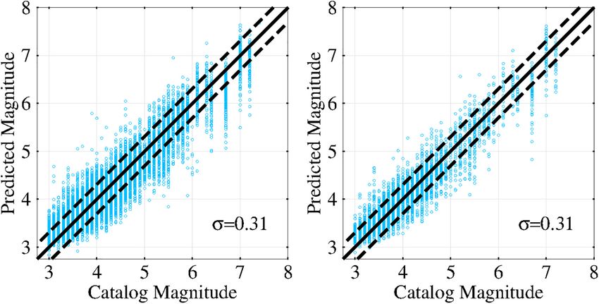
Zhu et al.                                                                                               Magnitude Estimation Using Neural Network

earthquake magnitudes. The τc method, which establishes the                 depths shallower than 10 km. We had no epicentral distance
empirical relationship between the average period (τc ) and                 requirements for the strong-motion data.
the CMs, was proposed by Kanamori (2005) and has been                          There were 1,836 inland earthquakes (Figure 1A)
demonstrated to have a relationship with the magnitude that is              characterized by 19,263 three-component seismograms recorded
acceptable for EEWSs (Wu and Kanamori, 2008; Yamada and                     by the K-NET stations (Figure 1B). The data were composed
Mori, 2009). Wu and Zhao (2006) proposed the Pd method,                     mainly of events within 3 ≤ MJMA ≤ 6.9 but included three
which establishes an empirical correlation between the peak                 MJMA 7 and MJMA 7.4 events (see Supplementary Table 1).
amplitude of displacement during the first 3 s after P-wave                 The P-wave arrival was determined automatically using the
arrival and the CMs and was applied to predict magnitudes in                short-term averaging/long-term averaging algorithm (Allen,
southern California. The Pd method provides robust magnitude                1978). Acceleration records were integrated once and twice to
estimation, and it is feasible to use the peak amplitude of                 obtain velocity and displacement seismograms, respectively.
displacement during the first several seconds after P-wave arrival          Then, the displacement seismograms were processed by using
to predict magnitudes for EEWSs (Zollo et al., 2006; Tsang et al.,          a Butterworth filter with a high-pass frequency of 0.075 Hz to
2007; Lin et al., 2011). The squared velocity integral (IV2), which         remove low-frequency drift (Wu and Zhao, 2006). Moreover,
was proposed by Festa et al. (2008), is related to the early radiated       selected seismic records were randomly divided into two
energy and can be used to determine earthquake magnitudes.                  datasets: a training dataset (15,410 three-component seismic
   However, since a single parameter might provide little                   records), which accounted for 80% of the strong-motion data,
magnitude information regardless of whether it is governed                  was used to train the DCNN-M model, and a test dataset (3,853
by the frequency, amplitude, or energy, the accuracy of                     three-component seismic records), which accounted for 20% of
EEW magnitude estimation still needs to be improved. More                   the strong-motion data, was used to assess the DCNN-M model
accurate magnitude estimation will lead to more effective                   performance after training (Figure 2).
hazard mitigation. With the development of artificial intelligence,
some researchers have combined magnitude estimation and
support vector machines (SVMs) and indicated that artificial                THE INPUT PARAMETERS
intelligence has excellent potential for use in EEW magnitude
estimation applications (Reddy and Nair, 2013; Ochoa et al.,                The P-wave parameters used to predict magnitude mainly include
2017). In this study, we developed an advanced magnitude                    three categories for EEW: parameters related to amplitude,
prediction model by using a deep convolutional neural network               frequency and energy. Since a single parameter provides little
for magnitude estimation (DCNN-M). Following the analyses                   earthquake magnitude information, multiple parameters might
by Kanamori (2005), Wu and Kanamori (2005), and Wu                          provide more information useful in magnitude prediction; thus,
and Zhao (2006), we also used the 3-s time window after                     for EEW, 12 magnitude estimation parameters of the P-wave
P-wave arrival for DCNN-M model estimation. We used 12                      arrival related to the frequency, amplitude, and energy are
magnitude estimation parameters from P-wave arrival for EEW                 selected as inputs to the DCNN-M model to make the DCNN-
related to the frequency, amplitude, and energy as input,                   M model interpretable. It is important that these 12 P-wave
which make the DCNN-M model interpretable, and trained                      parameters are correlated with magnitude in this paper. In this
the DCNN-M model using the training dataset. Then, the test                 study, these P-wave parameters are introduced in the following
dataset was used to test the DCNN-M model performance,                      paragraphs. Following the analysis of Kanamori (2005), Wu and
and DCNN-M model magnitude estimates were compared to                       Kanamori (2005), Wu and Zhao (2006), we also used the 3-s
the τc method and Pd method results. Furthermore, as a                      time window after P-wave arrival for DCNN-M model magnitude
test, we used the DCNN-M model to predict 31 additional                     estimation. Furthermore, we corrected the parameters related
earthquake events and obtained reliable magnitude estimates.                to amplitude, energy and derivative parameters for the distance
We show that the DCNN-M model is robust enough to predict                   effect by normalizing them to a reference distance of 10 km
magnitudes in Japan and that it has considerable potential for              (Zollo et al., 2006).
application to EEWSs.                                                           First, P-wave parameters related to amplitude include peak
                                                                            displacement (Pd ), peak velocity (Pv ), and peak acceleration
                                                                            (Pa ), which provide information on the earthquake size and
DATA AND PROCESSING                                                         these amplitude-related parameters have relationships with the
                                                                            magnitude (Wu and Kanamori, 2005; Wu and Zhao, 2006). The
In this study, we used strong-motion data from October 2007                 single data points for the P-wave parameters related to amplitude
through October 2017, which were obtained from the Kyoshin                  as a function of magnitude are shown in Supplementary
Network (K-NET) stations of the National Research Institute for             Figure 1. In addition, these parameters are defined as:
Earth Science and Disaster Prevention (NIED) in Japan1 (Aoi
et al., 2011). The sampling rate of the strong-motion data was                                     Pd = max dud (t)                             (1)
                                                                                                        0≤t≤T
100 Hz. We selected inland earthquakes from the K-NET catalog
with magnitudes within the 3 ≤ MJMA ≤ 8 range and focal                                            Pv = max |vud (t)|                           (2)
                                                                                                        0≤t≤T

1                                                                                                  Pa = max |aud (t)|                           (3)
    http://www.kyoshin.bosai.go.jp/                                                                     0≤t≤T

Frontiers in Earth Science | www.frontiersin.org                        2                                       May 2021 | Volume 9 | Article 653226
Zhu et al.                                                                                                                        Magnitude Estimation Using Neural Network

  FIGURE 1 | (A) The epicenter locations of the 1,836 inland earthquakes used in this paper. Solid red circles of different sizes indicate magnitudes within the range of
  3 ≤ MJMA ≤ 7.4. (B) The distribution of the stations (solid blue triangles) that recorded the strong-motion data used in this paper.

where dud (t), vud (t), and aud (t) are the vertical components of                       related to frequency as a function of magnitude are shown in
the displacement, velocity, and acceleration time histories of                           Supplementary Figure 2. In this paper, the linear relationship
the strong-motion data, respectively. Zero is the P-wave arrival                         between the frequency parameters and the magnitude is shown
time, and T is the length of the P-wave time window. In this                             in Supplementary Table 5.
paper, the linear relationship between the amplitude parameters,                            Finally, P-wave parameters related to the power of earthquakes
the magnitude and the hypocentral distance is shown in                                   include the P-wave index value (PIv ) (Nakamura, 2003), velocity
Supplementary Table 3, and the linear relationship between the                           squared integral (IV2) (Festa et al., 2008) and cumulative absolute
amplitude parameters after normalization to a reference distance                         velocity (CAV) (Reed and Kassawara, 1988; Böse, 2006). The
of 10 km and magnitude is shown in Supplementary Table 4.                                single data points for the P-wave parameters related to energy as
   Next, the P-wave parameters related to frequency include the                          a function of magnitude are shown in Supplementary Figure 3.
average period (τc ), product parameter (TP), and peak ratio                             In addition, these parameters are calculated as:
(Tva ). The average period has been proven to have an acceptable
relationship with the magnitude (Kanamori, 2005) and it can be                                             PI v = max log |aud (t) · vud (t)|                            (8)
                                                                                                                   0≤t≤T
calculated as:
                               RT 2
                                                                                                                    Z     T
                                                                                                                               2
                                   v (t) dt                                                                IV2 =              vud (t) dt                                 (9)
                          r = R 0T ud                          (4)                                                    0
                                 0 dud (t) dt
                                     2
                                                                                                                      Z     T
                                    2π                                                                     CAV =                |a3 (t)| dt                            (10)
                               τc = √                                          (5)                                      0
                                      r                                                                                 q
                                                                                                           a3 (t) =      a2ud (t) + a2ew (t) + a2ns (t)                (11)
The correlation of TP and magnitude was proposed by Huang
et al. (2015), which has correlations with τc and Pd , and TP is
                                                                                         where a3 (t) is the total acceleration of the three components. In
defined as:
                                                                                         this paper, the linear relationship between the energy parameters,
                         TP = τc × Pd                        (6)
                                                                                         the magnitude and the hypocentral distance is shown in
where τc is the average period and Pd is the peak displacement.                          Supplementary Table 6, and the linear relationship between the
The peak ratio reflects the frequency components of the ground                           energy parameters after normalization to a reference distance
motion and has a correlation with magnitude (Böse, 2006; Ma,                             of 10 km and magnitude is shown in Supplementary Table 7.
2008), which has correlations with Pv and Pa , and it can be                             Because, CAV considers the influence of both the amplitude and
calculated as:                                                                           the duration of motion, we proposed three derivative parameters
                        Tva = 2π (Pv /Pa )                  (7)                          according to the CAV. They are cumulative vertical absolute
                                                                                         displacement(cvad), cumulative vertical absolute velocity(cvav)
where Pv and Pa are the peak velocity and peak acceleration,                             and cumulative vertical absolute acceleration(cvaa). The single
respectively. The single data points for the P-wave parameters                           data points for the derivative parameters as a function of

Frontiers in Earth Science | www.frontiersin.org                                     3                                                   May 2021 | Volume 9 | Article 653226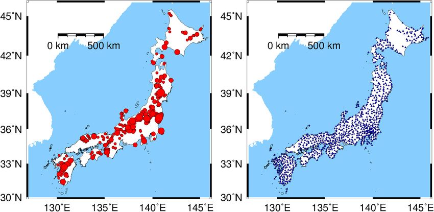
Zhu et al.                                                                                                               Magnitude Estimation Using Neural Network

  FIGURE 2 | The distribution of the epicentral distance and magnitude records. A histogram for the number of selected seismic records with the magnitude is shown
  at the top. An interval of 0.5 is used for each magnitude bin. A histogram of the number of selected seismic records with the epicentral distance is shown at the
  bottom left. An interval of 25 km is used for each epicentral distance bin. The distribution between the magnitude and epicentral distance is shown at the bottom
  right. Solid blue circles indicate the training dataset used to train the DCNN-M model. Solid red circles indicate the test dataset used to test the DCNN-M model
  performance.

magnitude are shown in Supplementary Figure 4. These                                      To prevent numerical problems caused by large variations
parameters are calculated as:                                                         between the ranges of the parameters and to improve the training
                                                                                      efficiency of the model, these parameters are linearly scaled to
                     cvad = sum dud (t)

                                                (12)                                  [−1, 1] as the input of the deep convolutional neural network
                                     0≤t≤T
                                                                                      (Tezcan and Cheng, 2012). When scaled to [−1, 1], every
                           cvav = sum (|vud (t)|)                          (13)       parameter becomes:
                                     0≤t≤T

                           cvaa = sum (|aud (t)|)                          (14)
                                     0≤t≤T                                                                            2x − (xmax + xmin )
                                                                                                           xnorm =                                              (15)
In this paper, the linear relationship between the derivative                                                            xmax − xmin
parameters, the magnitude and the hypocentral distance is
shown in Supplementary Table 8, and the linear relationship                           where xnorm is the original P-wave parameter and xmax and
between the derivative parameters after normalization to a                            xmin are the maximum and minimum values of every P-wave
reference distance of 10 km and magnitude is shown in                                 parameter extracted from the strong-motion data in this
Supplementary Table 9.                                                                study, respectively.

Frontiers in Earth Science | www.frontiersin.org                                  4                                             May 2021 | Volume 9 | Article 653226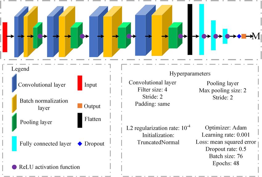
Zhu et al.                                                                                                               Magnitude Estimation Using Neural Network

THE DCNN-M MODEL                                                                     the hyperparameters freer, the network convergence speed
                                                                                     faster, and the performance better (Ioffe and Szegedy, 2015).
Earthquake early warning magnitudes are usually predicted                            A pooling layer followed each batch normalization layer;
via the empirical relationship between a single parameter                            we used max pooling, each max pooling size was 2, each
extracted from the seismic data collected during the first                           stride was 2, and each padding type was “same.” The final
few seconds after P-wave arrival and CMs. Since a single                             pooling layer was flattened and then fed to the first fully
parameter provides little earthquake magnitude information,                          connected layer. The three fully connected layers had 250,
multiple parameters might provide more information useful                            125, and 60 neurons.
in magnitude prediction. In addition, to make the model                                  To prevent overfitting and ensure better generalizability,
interpretable, for EEW, we used 12 magnitude estimation                              we applied L2 regularization with a regularization rate of
parameters related to the amplitude, frequency, and energy                           10−4 to the convolutional layers and dropout with a dropout
following the P-wave arrival (see Supplementary Text 1) as the                       rate of 0.5 following the last fully connected layer (Srivastava
inputs of the DCNN-M model.                                                          et al., 2014; Jozinović et al., 2020). Moreover, the rectified
    The DCNN-M model was constructed based on a deep                                 linear unit (ReLU) activation function (Nair and Hinton, 2010)
convolutional neural network and was used to predict                                 followed each pooling layer and fully connected layer. Because
magnitudes for EEW. The architecture of the DCNN-M                                   larger batch sizes lead to worse generalization performance
model comprised 12 parameters extracted from the 3 s period                          (Keskar et al., 2016), we used 76 batch sizes and 48 epochs
after P-wave arrival as inputs, four convolutional layers, four                      based on a tradeoff between efficiency and generalizability.
batch normalization layers, four pooling layers, three fully                         We used a training dataset to train the DCNN-M model
connected layers, and an output (Figure 3). The output was                           based on the Adam optimizer with a learning rate of 0.001
the predicted magnitude (PM). The four convolutional layers                          by optimizing a loss function defined as the mean squared
had 124, 150, 190, and 250 filters. In each convolutional layer,                     error of the output (Kingma and Ba, 2014). In this study,
the kernel size of the filter was 4, the stride was 2, the padding                   the DCNN-M model was programmed using TensorFlow
type was “same,” and the initialization was “TruncatedNormal.”                       GPU 2.3 and trained using the training dataset, requiring
A batch normalization layer followed each convolutional                              approximately 1.5 min on an Nvidia Quadro T1000 GPU
layer. The batch normalization layers made the setting of                            with 12 GB memory.

  FIGURE 3 | The architecture of the DCNN-M model. Twelve parameters related to the frequency, amplitude, and energy extracted from the 3-s period after P-wave
  arrival are used as the inputs of the DCNN-M model. The hyperparameters of the DCNN-M model include the filter size, stride, padding, initialization, optimizer,
  learning rate, regularization, and dropout, etc.

Frontiers in Earth Science | www.frontiersin.org                                 5                                              May 2021 | Volume 9 | Article 653226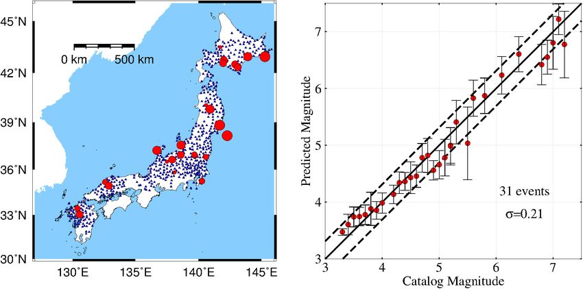
Zhu et al. Magnitude Estimation Using Neural Network
RESULTS for magnitude estimation by the τc method and Pd method are
given by:
In this study, the difference between the PM and CM is defined as
the error (ω). The error (ω) and the standard deviation (σ) of the log (τc ) = −1.07 (±0.02) + 0.19(±0.01)M (18)
errors are expressed as:
log Pd10km = −4.84 (±0.02) + 0.78(±0.01)M (19)
ω = PM − CM (16)
v
u
u1 X N Compared to the DCNN-M model results, the magnitude
σ=t (ωi − $ )2 (17) estimation results from the τc method and Pd method exhibit
N considerable scatter. The standard deviations of the magnitude
i=1
estimation error are 1.56, 0.42, and 0.31 for the τc method, Pd
where N is the number of records and $ is the mean of the errors. method, and DCNN-M model, respectively. There is obvious
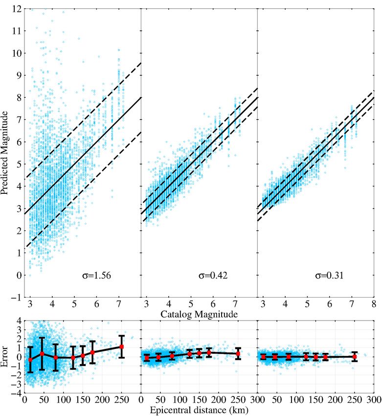
Figure 4 depicts magnitude estimation for the training magnitude overestimation (MJMA ≤ 5) from the τc method and
dataset (Figure 4A) and the test dataset (Figure 4B) based Pd method, but this issue is improved considerably in the DCNN-
on the DCNN-M model. The PMs approximate the CMs in M model results. The magnitudes predicted by the DCNN-M
the training and test datasets. The standard deviations of the model are closer to the vs. than those from the τc method and
magnitude estimation errors are 0.31 for both the training Pd method.
and test datasets. This finding indicates excellent generalization Furthermore, the variation in the magnitude estimation error
performance and an absence of overfitting within the DCNN- with the epicentral distance is presented in Figure 5 for the
M model. τc method (Figure 5D), Pd method (Figure 5E), and DCNN-
The τc method and Pd method are widely used in the M model (Figure 5F). It can be observed from the distribution
study of EEWS magnitude prediction (Kanamori, 2005; of circles that the τc method and Pd method exhibit larger
Wu and Kanamori, 2005; Wu and Zhao, 2006; Zollo errors than the DCNN-M model. In addition, the magnitude
et al., 2006; Colombelli et al., 2014). To evaluate the estimation errors from the τc method and Pd method have larger
performance of the DCNN-M model, the τc method and discreteness (black bars) than those from the DCNN-M model,
Pd method were used to predict the magnitudes, and the and the means (red squares) of the magnitude estimation errors
results were compared. from the τc method and Pd method clearly vary with increasing
For the same test dataset and the 3-s time window after P-wave epicentral distance. This phenomenon is especially true for the
arrival, Figures 5A–C show the τc method, Pd method, and τc method. The mean (red square) of the DCNN-M model
DCNN-M model estimation results, respectively. The magnitude magnitude estimation errors is nearly zero, and the DCNN-
estimates of the τc method and Pd method are obtained based on M model magnitude estimation errors are not affected by the
Supplementary Tables 4, 5, respectively. The relationships used epicentral distance.
FIGURE 4 | Correlations between the predicted and catalog magnitudes. (A) Magnitude estimation for the training dataset used to train the DCNN-M model. (B) The
magnitude estimation of the test dataset used to test the DCNN-M model performance. When a data point is on the solid black 45◦ line, the predicted magnitude is
equal to the catalog magnitude. The two black dashed lines indicate the range of one standard deviation of error.
Frontiers in Earth Science | www.frontiersin.org 6 May 2021 | Volume 9 | Article 653226Zhu et al. Magnitude Estimation Using Neural Network FIGURE 5 | Catalog magnitudes versus predicted magnitudes produced using the test dataset by (A) the τc method, (B) the Pd method, and (C) the DCNN-M model. On the solid black 45◦ line, the predicted magnitude is equal to the catalog magnitude. The two black dashed lines indicate the locations of one standard deviation of error. The relationship between the epicentral distance and the error in the predicted magnitude for (D) the τc method, (E) the Pd method, and (F) the DCNN-M model. The epicentral distance is divided into seven sections: (0 km, 30 km), (30 km, 60 km), (60 km, 100 km), (100 km, 150 km), (125 km, 175 km), (150 km, 200 km), and (200 km, 200+ km). The position of the solid red square represents the mean of the errors within an epicentral distance. The length of the black bar shows the standard deviation of the magnitude estimation errors within an epicentral distance, which reflects the discreteness of the errors. For a given test dataset, Table 1 compares the distribution DCNN-M model is more accurate than the τc method and Pd of the magnitude estimation absolute errors for the τc method, method and has considerable EEW application potential. Pd method, and DCNN-M model. As shown in Table 1, the absolute magnitude estimation errors of the DCNN-M model are concentrated mainly in the range of 0.6 magnitude units of OFFLINE APPLICATION OF THE approximately 2σ, and the results for the DCNN-M model are DCNN-M MODEL nearly 60 and 10% greater than those of the τc method and Pd method, respectively, in the range of 0.6 magnitude units. To test the robustness of the DCNN-M model in analyzing new Moreover, for the absolute magnitude estimation errors greater earthquake events, we tested the magnitude prediction of 31 than 1.2 magnitude units, the percentage of DCNN-M model additional events. These events were not included in the training results is nearly zero and is much less than those from the τc and test datasets. These events (see Supplementary Table 2) method and Pd method. These analyses also indicate that the occurred mainly between April 2018 and December 2019. Due Frontiers in Earth Science | www.frontiersin.org 7 May 2021 | Volume 9 | Article 653226
Zhu et al.                                                                                                                    Magnitude Estimation Using Neural Network

TABLE 1 | The distribution of the magnitude estimation errors for the τc method,        (Kanamori, 2005; Wu and Kanamori, 2005; Wu and Zhao, 2006;
Pd method, and DCNN-M model.
                                                                                        Zollo et al., 2006; Colombelli et al., 2014). Since a single parameter
Absolute error range                       Percentage of records                        might provide little magnitude information, we introduce an
                                                                                        advanced magnitude prediction model named DCNN-M in this
                             τ c method            Pd method         DCNN-M             paper. DCNN-M uses a deep convolutional neural network to
                                 (%)                  (%)            model (%)          perform magnitude estimation. We used a training dataset to
0 ≤ | error| ≤ 0.6              34.13                86.71              94.78           train the DCNN-M model and 12 parameters extracted from
0.6 < | error| ≤ 1.2            27.82                12.30               4.98           the initial 3 s of the P-wave record as inputs to the DCNN-M
1.2 < | error|                  38.05                0.99                0.24           model. These parameters are related to the frequency, amplitude,
                                                                                        and energy, which make the DCNN-M model interpretable.
                                                                                        Additionally, although many of these input parameters might not
to the small number of large earthquakes with MJMA ≥ 6 in this                          be independent of each other, they are not completely the same,
time period, we also selected seven earthquakes with MJMA ≥ 6                           and more parameters might provide more information about the
that occurred before October 2007. The distribution of stations                         magnitude. In addition, a test dataset was used to test the DCNN-
and epicenters for the 31 events and the magnitude prediction for                       M model performance. The results were compared to those from
these events are shown in Figures 6A,B, respectively. The solid                         the τc method and Pd method. As a further test, we used the
red circle shows the mean estimated magnitude of the DCNN-                              DCNN-M model to predict 31 additional events.
M model for an earthquake event. The PMs of these events are                               In this study, we used 1,836 inland earthquakes from the
quite similar to the CMs, and nearly all of the PMs are within the                      K-NET catalog with magnitudes in the 3 ≤ MJMA ≤ 7.2 range and
standard deviation (0.31) of the errors for the DCNN-M model.                           focal depths shallower than 10 km. To use more accurate P-wave
In addition, the standard deviation of the errors for these events                      arrival information, first, we use the short-term averaging/long-
is 0.21. Moreover, reliable results without obvious magnitude                           term averaging algorithm (Allen, 1978) to determine the P-wave
overestimation and underestimation are obtained for events with                         arrival automatically. Then compared with the P-wave arrival
MJMA ≤ 7.2.                                                                             determined manually, the records that have a larger difference
                                                                                        between the P-wave arrival determined automatically and the
                                                                                        P-wave arrival determined manually are discarded. For the
DISCUSSION AND CONCLUSION                                                               test dataset, DCNN-M magnitude estimation provided smaller
                                                                                        errors and no obvious overall magnitude underestimation or
For the past several decades, EEW magnitudes have been                                  overestimation relative to the τc method and Pd method. In
determined by establishing regression functions between a single                        principle, the DCNN-M model can be extended to earthquakes
P-wave parameter and the CMs. The τc method and Pd method                               in other regions. We plan to test it with strong-motion data from
have been widely used in the study of EEW magnitude estimation                          China because most earthquakes in China are inland earthquakes

  FIGURE 6 | (A) The distribution of the epicenter locations and stations for 31 additional earthquakes. The solid red circles of different sizes represent magnitudes of
  3 ≤ MJMA ≤ 7.2. The solid blue triangles represent stations that recorded the 31 events. (B) Magnitudes determined using the DCNN-M model versus the catalog
  magnitudes for the 31 additional events. On the solid black 45◦ line, the predicted magnitude is equal to the catalog magnitude. The two black dashed lines indicate
  the locations (0.31) of the one standard deviation of errors for the DCNN-M model. The solid red circles show the mean of the estimated magnitudes of the DCNN-M
  model for the earthquake events. The length of the black bar shows the standard deviation of the magnitude estimation errors for each event.

Frontiers in Earth Science | www.frontiersin.org                                    8                                               May 2021 | Volume 9 | Article 653226
Zhu et al. Magnitude Estimation Using Neural Network with focal depths shallower than 10 km (Song et al., 2018). In Importantly in this study, we corrected the parameters related this study, the problem of the possible underestimation of large to amplitude, energy and derivative parameters for the distance earthquakes did not appear in the dataset of earthquakes with effect by normalizing them to a reference distance of 10 km magnitudes in the 3 ≤ MJMA ≤ 7.2 range. The problem of (Zollo et al., 2006). In our application, based on real-time underestimation of large earthquakes (MJMA ≥ 7.5) remains to earthquake locations provided by an EEWS, the magnitude be studied. Extending the training dataset magnitude range or estimation of the DCNN-M model is determined. The method the time window after P-wave arrival may solve problems related used to determine real-time earthquake locations is similar to to larger (MJMA ≥ 7.5) earthquakes (Colombelli et al., 2012; that of Zollo et al. (2010), which was developed by Satriano Chen et al., 2017). et al. (2008). Moreover, it also provides the possibility to detect The DCNN-M model trained using the training dataset could earthquake locations based on the deep learning method (Perol provide ideal test dataset magnitude estimation results. The et al., 2018; Zhang et al., 2019, 2020) and has potential for future standard deviations of the magnitude estimation errors of the application in EEW. training and test datasets were both 0.31. This finding indicates However, the DCNN-M model hyperparameters, the size of that the DCNN-M model provided good generalizability with the training dataset and the input parameters are also important no overfitting. Our results show that the magnitudes predicted in magnitude estimation. The hyperparameters include the by the DCNN-M model, which provided a standard deviation number of layers, number of filters, dropout rate, optimizer, of 0.31 based on the 3-s time window after P-wave arrival, learning rate, batch size, and stride. In this paper, we tried exhibited better agreement with the CMs than the magnitudes several times to debug each hyperparameter of the DCNN-M predicted using the τc method and Pd method, which provided model manually to identify those hyperparameters that might not standard deviations of 1.56 and 0.42, respectively. In addition, the be optimal. However, the comparison of the DCNN-M model magnitude estimates from the τc method provided considerable magnitude estimates with those produced via the τc method and scatter and overestimation at MJMA ≤ 5. These phenomena Pd method indicated that the DCNN-M model has considerable are consistent with the results of Carranza et al. (2015). In potential for EEW applications and provides robust magnitude contrast, the PMs from the DCNN-M model significantly estimation. In this study, we use 12 parameters extracted from approximate the CMs. The τc parameter is used as an input to the initial 3 s of the P-wave record as inputs to the DCNN-M the DCNN-M model, but there is no significant overestimation model, and we may find that more parameters with magnitude at MJMA ≤ 5. The reason may be that the DCNN-M model information could be used as the input of the DCNN-M model in training reduces the influence of τc on the model magnitude, the future. To improve the performance of the DCNN-M model and the correlation between the frequency content of the τc with regard to the magnitude estimation accuracy, the DCNN- parameter and magnitude is learned. The magnitude estimates M model hyperparameters and the input parameters need to be from the DCNN-M model were not affected by the epicentral optimized, and the amount of strong-motion data still needs to be distance, unlike those of the τc method and Pd method. expanded (Perol et al., 2018). The DCNN-M model will be more For the same test dataset, the absolute magnitude estimation effective at avoiding false EEW alarms than the τc method and errors of the DCNN-M model are mainly concentrated in Pd method. the range of 0.6 magnitude units at approximately 2σ, and the percentage of the magnitude estimation error is 94.78% greater than those of the τc method and Pd method. This DATA AVAILABILITY STATEMENT finding means that the DCNN-M model has better magnitude determination performance than the τc method and Pd method, The original contributions presented in the study are included and the probability that the magnitude estimation error is in the article/Supplementary Material, further inquiries can be in the range of 0.6 magnitude units is 94.78%. Furthermore, directed to the corresponding author. we obtained reliable magnitude estimates without obvious magnitude overestimation and underestimation for 31 additional events using the DCNN-M model. These results indicate that the AUTHOR CONTRIBUTIONS DCNN-M model has considerable EEW magnitude estimation application potential in Japan. JZ implemented and applied the method and wrote the related In Japan, magnitude is measured with the magnitude scale text. JS contributed to designing the methodology and revised MJMA ; hence, the magnitude scale MJMA is used as the target the manuscript. SL and YW provided important suggestions for predicted by the DCNN-M model for the area of Japan in this the interpretation of the results. All authors contributed to the paper. For different magnitude scales and user requirement, redaction and final revision of the manuscript. we could use the conversion relationship between different magnitude scales or use a different magnitude scale (likely Mw ) as the target predicted by the DCNN-M model. Different magnitude FUNDING scales might influence our results. We mainly propose a new magnitude model (DCNN-M) for magnitude determination in This research was financially supported by the National this paper for EEW. In the next step we will deeply study the Key Research and Development Program of China influence of different magnitude scales on the DCNN-M model. (2018YFC1504003) and its provincial funding, the National Frontiers in Earth Science | www.frontiersin.org 9 May 2021 | Volume 9 | Article 653226
Zhu et al.                                                                                                                            Magnitude Estimation Using Neural Network

Natural Science Foundation of China (51408564 and U1534202),                                   station strong-motion data. We are also grateful for the GMT
and the Scientific Research Fund of Institute of Engineering                                   software used by Wessel and Smith (1988).
Mechanics, China Earthquake Administration (2016A03).

                                                                                               SUPPLEMENTARY MATERIAL
ACKNOWLEDGMENTS
                                                                                               The Supplementary Material for this article can be found
We thank the National Research Institute for Earth Science and                                 online at: https://www.frontiersin.org/articles/10.3389/feart.
Disaster Prevention (NIED), Japan, for providing the K-NET                                     2021.653226/full#supplementary-material

REFERENCES                                                                                        convolutional neural network. Geophys. J. Int. 222, 1379–1389. doi: 10.1093/
                                                                                                  gji/ggaa233
Allen, R. M., Brown, H., Hellweg, M., Khainovski, O., Lombard, P., and Neuhauser,              Kanamori, H. (2005). Real–time seismology and earthquake damage mitigation.
    D. (2009a). Real–time earthquake detection and hazard assessment by ElarmS                    Annu. Rev. Earth Planet Sci. 33, 195–214. doi: 10.1146/annurev.earth.33.
    across California. Geophys. Res. Lett 36:L00B08. doi: 10.1029/2008gl036766                    092203.122626
Allen, R. M., Gasparini, P., Kamigaichi, O., and Böse, M. (2009b). The status of               Keskar, N. S., Mudigere, D., Nocedal, J., Smelyanskiy, M., and Tang, P. T. P. (2016).
    earthquake early warning around the world: an introductory overview. Seismol.                 On Large–Batch Training for Deep Learning: Generalization Gap and Sharp
    Res. Lett. 80, 682–693. doi: 10.1785/gssrl.80.5.682                                           Minima arXiv [Preprint]. Available online at: http://arxiv.org/abs/1609.04836
Allen, R. M., and Kanamori, H. (2003). The potential for earthquake early warning                 (accessed September 2020).
    in Southern California. Science 300, 786–789. doi: 10.1126/science.1080912                 Kingma, D. P., and Ba, J. (2014). Adam: A Method for Stochastic Optimization
Allen, R. V. (1978). Automatic earthquake recognition and timing from single                      arXiv [Preprint]. available online at: http://arxiv.org/abs/1412.6980 (accessed
    traces. Bull. Seismol. Soc. Am. 68, 1521–1532. doi: 10.1007/BF02247958                        November 2020).
Aoi, S., Kunugi, T., Nakamura, H., and Fujiwara, H. (2011). Deployment of                      Lin, T. L., Wu, Y. M., and Chen, D. Y. (2011). Magnitude estimation using initial
    New Strong Motion Seismographs of K–NET and KiK–net. Berlin: Springer                         P–wave amplitude and its spatial distribution in earthquake early warning in
    Netherlands Press.                                                                            Taiwan. Geophys. Res. Lett. 38:L09303. doi: 10.1029/2011gl047461
Aranda, J. M. E., Jiménez, A., Ibarrola, G., Alcantar, F., Aguilar, A., Inostroza, M.,         Ma, Q. (2008). Study and Application on Earthquake Early Warning [Ph.D. thesis].
    et al. (1995). Mexico city seismic alert system. Seismol. Res. Lett. 66, 42–53.               Harbin: Institute of engineering mechanics.
    doi: 10.1785/gssrl.66.6.42                                                                 Nair, V., and Hinton, G. E. (2010). “Rectified linear units improve restricted
Böse, M. (2006). Earthquake Early Warning for Istanbul Using Artificial Neural                    boltzmann machines,” in Proceedings of the 27th International Conference on
    Networks [Ph.D. thesis]. Karlsruhe: University of Karlsruhe.                                  International Conference on Machine Learning (ICML-10) (Haifa: Omnipress).
Carranza, M., Buforn, E., and Zollo, A. (2015). Testing the earthquake early–                  Nakamura, Y. (2003). “A new concept for the earthquake vulnerability estimation
    warning parameter correlations in the Southern Iberian Peninsula. Pure Appl.                  and its application to the early warning system,” in Early Warning Systems for
    Geophys. 172, 2435–2448. doi: 10.1007/s00024-015-1061-6                                       Natural Disaster Reduction, eds J. Zschau and A. Küppers (Berlin: Springer-
Chen, D. Y., Hsiao, N. C., and Wu, Y. M. (2015). The earthworm based earthquake                   Verlag).
    alarm reporting system in Taiwan. Bull. Seismol. Soc. Am. 105, 568–579. doi:               Ochoa, L. H., Niño, L. F., and Vargas, C. A. (2017). Fast magnitude determination
    10.1785/0120140147                                                                            using a single seismological station record implementing machine learning
Chen, D. Y., Wu, Y. M., and Chin, T. L. (2017). An empirical evolutionary                         techniques. Geod. Geodyn. 9, 34–41. doi: 10.1016/j.geog.2017.03.010
    magnitude estimation for early warning of earthquakes. J. Asian. Earth Sci. 135,           Olson, E. L., and Allen, R. M. (2005). The deterministic nature of earthquake
    190–197. doi: 10.1016/j.jseaes.2016.12.028                                                    rupture. Nature 438, 212–215. doi: 10.1038/nature04214
Colombelli, S., Carotenuto, F., Elia, L., and Zollo, A. (2020). Design and                     Perol, T., Gharbi, M., and Denolle, M. (2018). Convolutional neural network
    implementation of a mobile device app for network–based earthquake early                      for earthquake detection and location. Sci. Adv. 4, 1–8. doi: 10.1126/sciadv.
    warning systems (EEWSs): application to the PRESTo EEWS in southern Italy.                    1700578
    Nat. Hazards Earth Syst. Sci. 20, 921–931. doi: 10.5194/nhess-20-921-2020                  Reddy, R., and Nair, R. R. (2013). The efficacy of support vector machines (SVM) in
Colombelli, S., Zollo, A., Festa, G., and Kanamori, H. (2012). Early magnitude and                robust determination of earthquake early warning magnitudes in central Japan.
    potential damage zone estimates for the great Mw 9 Tohoku–Oki earthquake.                     J. Earth Syst. Sci. 122, 1423–1434. doi: 10.1007/s12040-013-0346-3
    Geophys. Res. Lett. 39:L22306. doi: 10.1029/2012gl053923                                   Reed, J. W., and Kassawara, R. P. (1988). A criterion for determining exceedance
Colombelli, S., Zollo, A., Festa, G., and Picozzi, M. (2014). Evidence for a difference           of the operating basis earthquake. Nucl. Eng. Des. 123, 387–396. doi: 10.1016/
    in rupture initiation between small and large earthquakes. Nat. Comm. 5:3958.                 0029-5493(90)90259-z
    doi: 10.1038/ncomms4958                                                                    Satriano, C., Lomax, A., and Zollo, A. (2008). Real-time evolutionary earthquake
Festa, G., Zollo, A., and Lancieri, M. (2008). Earthquake magnitude estimation                    location for seismic early warning. Bull. seism. Soc. Am. 98, 1482–1494. doi:
    from early radiated energy. Geophys. Res. Lett. 35:L22307. doi: 10.1029/                      10.1785/0120060159
    2008gl035576                                                                               Song, J. D., Jiao, C. C., Li, S. Y., and Hou, B. R. (2018). Prediction method of
Heidari, R., Shomali, Z. H., and Ghayamghamian, M. R. (2012). Magnitude–scaling                   first–level earthquake warning for high speed railway based on two–parameter
    relations using period parameters τc and τpmax, for Tehran region. Iran.                      threshold of seismic P–wave. China Railw. Sci. 39, 138–144. (in Chinese),
    Geophys. J. Int. 192, 275–284. doi: 10.1093/gji/ggs012                                     Srivastava, N., Hinton, G., Krizhevsky, A., Sutskever, I., and Salakhutdinov, R.
Hoshiba, M., Kamigaichi, O., Saito, M., Tsukada, S., and Hamada, N. (2008).                       (2014). Dropout: a simple way to prevent neural networks from overfitting.
    Earthquake early warning starts nationwide in Japan. Eos. Trans. Am. Geophys.                 J. Mach. Learn. Res. 15, 1929–1958.
    Union 89, 73–74. doi: 10.1029/2008EO080001                                                 Tezcan, J., and Cheng, Q. (2012). Support vector regression for estimating
Huang, P. L., Lin, T. L., and Wu, Y. M. (2015). Application of τc∗ Pd in earthquake               earthquake response spectra. B Earthq. Eng. 10, 1205–1219. doi: 10.1007/
    early warning. Geophys. Res. Lett. 42, 1403–1410. doi: 10.1002/2014gl06                       s10518-012-9350-2
    3020                                                                                       Tsang, L. L. H., Allen, R. M., and Wurman, G. (2007). Magnitude scaling relations
Ioffe, S., and Szegedy, C. (2015). Batch normalization: Accelerating Deep Network                 from P–waves in southern California. Geophys. Res. Lett. 34:L19304. doi: 10.
    Training by Reducing Internal Covariate Shift arXiv [Preprint]. Available online              1029/2007gl031077
    at http://arxiv.org/abs/1502.03167 (accessed September 2020).                              Wu, Y. M., and Kanamori, H. (2005). Rapid assessment of damage potential of
Jozinović, D., Lomax, A., Štajduhar, I., and Michelini, A. (2020). Rapid prediction              earthquakes in Taiwan from the beginning of P waves. Bull. Seismol. Soc. Am.
    of earthquake ground shaking intensity using raw waveform data and a                          95, 1181–1185. doi: 10.1785/0120040193

Frontiers in Earth Science | www.frontiersin.org                                          10                                                 May 2021 | Volume 9 | Article 653226
Zhu et al. Magnitude Estimation Using Neural Network Wu, Y. M., and Kanamori, H. (2008). Development of an earthquake early warning and performance evaluation. Geophys. Res. Lett. 36:L00B07. doi: 10.1029/ system using real–time strong motion signals. Sensors Basel 8, 1–9. doi: 10.3390/ 2008GL036689 s8010001 Zollo, A., Lancieri, M., and Nielsen, S. (2006). Earthquake magnitude estimation Wu, Y. M., and Teng, T. L. (2002). A virtual subnetwork approach to earthquake from peak amplitudes of very early seismic signals on strong motion records. early warning. Bull. Seismol. Soc. Am. 92, 2008–2018. doi: 10.1785/0120010217 Geophys. Res. Lett. 33:L23312. doi: 10.1029/2006gl027795 Wu, Y. M., and Zhao, L. (2006). Magnitude estimation using the first three seconds Zollo, A., Ortensia, A., Maria, L., Wu, Y. M., and Kanamori, H. (2010). A threshold- P–wave amplitude in earthquake early warning. Geophys. Res. Lett. 33:L16312. based earthquake early warning using dense accelerometer networks. Geophys J doi: 10.1029/2006gl026871 Int 183, 963–974. doi: 10.1111/j.1365-246X.2010.04765.x Yamada, M., and Mori, J. (2009). Using τc to estimate magnitude for earthquake early warning and effects of near–field terms. J. Geophys. Res. 114:B05301. Conflict of Interest: The authors declare that the research was conducted in the doi: 10.1029/2008jb006080 absence of any commercial or financial relationships that could be construed as a Zhang, M., Ellsworth, W. L., and Beroza, G. C. (2019). Rapid earthquake potential conflict of interest. association and location. Seismol. Res. Lett. 90, 2276–2284. doi: 10.1785/ 0220190052 Copyright © 2021 Zhu, Li, Song and Wang. This is an open-access article distributed Zhang, X., Zhang, J., Yuan, C., Liu, S., Chen, Z., and Li, W. (2020). Locating induced under the terms of the Creative Commons Attribution License (CC BY). The use, earthquakes with a network of seismic stations in Oklahoma via a deep learning distribution or reproduction in other forums is permitted, provided the original method. Sci. Rep. 10:1941. doi: 10.1038/s41598-020-58908-5 author(s) and the copyright owner(s) are credited and that the original publication Zollo, A., Iannaccone, G., Lancieri, M., Cantore, L., Convertito, V., Emolo, A., in this journal is cited, in accordance with accepted academic practice. No use, et al. (2009). Earthquake early warning system in southern Italy: Methodologies distribution or reproduction is permitted which does not comply with these terms. Frontiers in Earth Science | www.frontiersin.org 11 May 2021 | Volume 9 | Article 653226
You can also read