Main-sequence galaxies across cosmic time
←
→
Page content transcription
If your browser does not render page correctly, please read the page content below
Astronomy & Astrophysics manuscript no. Wang_etal_2020                                                                               ©ESO 2022
                                               January 31, 2022

                                                  A3 COSMOS: A census on the molecular gas mass and extent of
                                                          main-sequence galaxies across cosmic time
                                                    Tsan-Ming Wang1 , Benjamin Magnelli1, 2 , Eva Schinnerer3 , Daizhong Liu4 , Ziad Aziz Modak1 , Eric Faustino
                                                               Jiménez-Andrade5 , Christos Karoumpis1 , Vasily Kokorev6, 7 , and Frank Bertoldi1

                                                     1
                                                         Argelander-Institut für Astronomie, Universität Bonn, Auf dem Hügel 71, 53121 Bonn, Germany
                                                         e-mail: twan@uni-bonn.de
                                                     2
                                                         AIM, CEA, CNRS, Université Paris-Saclay, Université Paris Diderot, Sorbonne Paris Cité, 91191 Gif-sur-Yvette, France
                                                     3
                                                         Max-Planck-Institut für Astronomie, Königstuhl 17, 69117 Heidelberg, Germany
                                                     4
                                                         Max-Planck-Institut für extraterrestrische Physik, Gießenbachstraße 1, 85748 Garching b. München, Germany
arXiv:2201.12070v1 [astro-ph.GA] 28 Jan 2022

                                                     5
                                                         National Radio Astronomy Observatory, 520 Edgemont Road, Charlottesville, VA 22903, USA
                                                     6
                                                         Cosmic Dawn Center (DAWN), Copenhagen, Denmark
                                                     7
                                                         Niels Bohr Institute, University of Copenhagen, Lyngbyvej 2, 2100 Copenhagen Ø, Denmark

                                                    Received xxx; accepted xxx

                                                                                                                 ABSTRACT

                                                    Aims. To constrain for the first time the mean mass and extent of the molecular gas of a mass-complete sample of normal > 1010 M
                                                    star-forming galaxies at 0.4 < z < 3.6.
                                                    Methods. We apply an innovative uv-based stacking analysis to a large set of archival Atacama Large Millimeter/submillimeter
                                                    Array (ALMA) observations using a mass-complete sample of main-sequence (MS) galaxies. This stacking analysis, performed on
                                                    the Rayleigh-Jeans dust continuum emission, provides accurate measurements of the mean mass and extent of the molecular gas of
                                                    galaxy populations, which are otherwise individually undetected.
                                                    Results. The molecular gas mass of MS galaxies evolves with redshift and stellar mass. At all stellar masses, the molecular gas
                                                    fraction decreases by a factor of ∼ 24 from z ∼ 3.2 to z ∼ 0. At a given redshift, the molecular gas fraction of MS galaxies decreases
                                                    with stellar mass, at roughly the same rate as their specific star formation rate (SFR/M? ) decreases. The molecular gas depletion time
                                                    of MS galaxies remains roughly constant at z > 0.5 with a value of 300–500 Myr, but increases by a factor ∼ 3 from z ∼ 0.5 to
                                                    z ∼ 0. This evolution of the molecular gas depletion time of MS galaxies can be predicted from the evolution of their molecular gas
                                                    surface density and a seemingly universal MS-only Σ Mmol − ΣSFR relation with an inferred slope of ∼ 1.13, i.e., the so-called Kennicutt-
                                                    Schmidt (KS) relation. The far-infrared size of MS galaxies shows no significant evolution with redshift or stellar mass, with a mean
                                                    circularized half-light radius of ∼2.2 kpc. Finally, our mean molecular gas masses are generally lower than previous estimates, likely
                                                    caused by the fact that literature studies were largely biased towards individually-detected MS galaxies with massive gas reservoirs.
                                                    Conclusions. To first order, the molecular gas content of MS galaxies regulates their star formation across cosmic time, while variation
                                                    of their star formation efficiency plays a secondary role. Despite a large evolution of their gas content and SFRs, MS galaxies evolved
                                                    along a seemingly universal MS-only KS relation.
                                                    Key words. galaxies: evolution – galaxies: high-redshift – galaxies: ISM

                                               1. Introduction                                                            Whitaker et al. 2014; Sobral et al. 2014; Speagle et al. 2014;
                                                                                                                          Johnston et al. 2015; Tomczak et al. 2016; Bourne et al. 2017;
                                               Understanding galaxy evolution across cosmic time is one of                Pearson et al. 2018; Popesso et al. 2019; Leslie et al. 2020). The
                                               the key topics of modern astronomy. To address this vast and               existence of the MS, with its constant scatter of 0.3 dex and a
                                               important question, one very successful approach is to assem-              normalisation that decreases by a factor of 20 from z ∼ 2 to
                                               ble and study large and representative samples of galaxies,                z ∼ 0, suggests that most star-forming galaxies (SFGs) are iso-
                                               through multi-wavelength deep extragalactic surveys. Using this            lated and secularly evolving with long (> Gyr) star-forming duty
                                               approach, much has been learned over the last decades about                cycles. On the contrary, galaxies above the MS (∼ 5% of the
                                               the global star formation history of the Universe. The cosmic              SFG population; Luo et al. 2014) seem to be mostly associated
                                               star formation rate density (SFRD) increases from early cosmic             to short, intense starbursts triggered by major mergers and con-
                                               times, z ∼ 2, and decreases by a factor of 10 by z ∼ 0 (Madau &            tribute only 10% to the SFRD at all redshifts (e.g., Sargent et
                                               Dickinson 2014). About 80% of this star formation takes place              al. 2012). While the evolution of the MS and SFRD across cos-
                                               in relatively massive galaxies (> 1010 M ) that reside on the              mic time is observationally well established up to z ∼ 2, the
                                               so-called main sequence (MS) of star-forming galaxies (e.g.,               mechanisms driving their evolution are yet poorly constrained.
                                               Noeske et al. 2007; Rodighiero et al. 2011; Sargent et al. 2012).          At z > 2, our understanding is even more limited because obser-
                                               This MS denotes the tight correlation existing between the stellar         vations obtained from different rest-frame frequencies (i.e., UV,
                                               mass (M? ) and star-formation rate (SFR) of galaxies which is ob-          far-infrared or radio) provide a somewhat discrepant view of the
                                               served up to z ∼ 4 (e.g., Brinchmann et al. 2004; Pannella et al.          exact evolution of the SFRD (e.g., Bouwens et al. 2015; Novak
                                               2009; Magdis et al. 2010; Zahid et al. 2012; Kashino et al. 2013;          et al. 2017; Liu et al. 2018; Gruppioni et al. 2020).

                                                                                                                                                                     Article number, page 1 of 27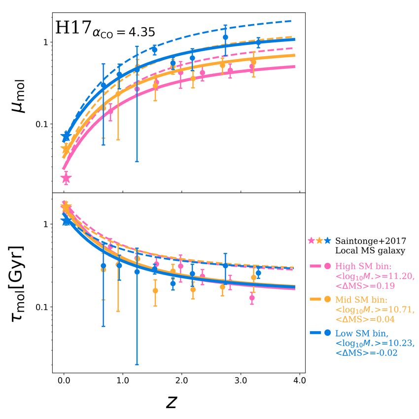
A&A proofs: manuscript no. Wang_etal_2020

     To shed light on the physical processes that regulate star for-   lying complex selection functions. Each sub-sample could thus
mation across cosmic time, it is paramount to obtain a precise         still fail to provide a complete, and representative view on the gas
measurement of the molecular gas content of local and high-            content of high-redshift galaxies. This likely explains in part why
redshift galaxies. Indeed, molecular gas fuels star formation, as      these studies agreed qualitatively but disagree quantitatively on
revealed by the tight correlation between gas mass and star for-       the exact redshift evolution of the gas content of massive galax-
mation rate surface densities, the so-called Kennicutt-Schmidt         ies (see Liu et al. 2019b). Finally, and most importantly, these
(KS) relation (Kennicutt 1998a). Molecular hydrogen (H2 ) is           studies relied mainly on individually-detected galaxies and were
the most abundant constituent of molecular gas, but it is dif-         thus limited to the high-mass end (> 1010.5 M ) of the SFG pop-
ficult to observe due to its lack of a dipole moment. For this         ulation. While constraining the gas content of massive galax-
reason, the carbon monoxide (CO) molecule, which is the most           ies is important, extending our knowledge towards lower stellar
abundant and readily observable constituent of molecular gas, is       masses is crucial because the bulk of the star formation activity
usually used to trace the molecular gas content of galaxies (see       of the Universe is known to take place in 1010···10.5 M galax-
Bolatto et al. 2013, for a review). However, even with the Ata-        ies (e.g., Karim et al. 2011; Leslie et al. 2020). The gas prop-
cama Large Millimeter/submillimeter Array (ALMA), obtaining            erties of these crucial low-mass high-redshift SFGs remain thus
such measurements for z > 2.0 MS galaxies with stellar mass            to date largely unknown simply because most are individually-
of ∼1010 M still requires an hour of observing time per object.        undetected even in deep ALMA observations.
Thus, the CO molecule is still poorly suited for the study of large         To statistically retrieve the faint emission of this SFG popu-
and representative samples of high-redshift galaxies. Therefore,       lation, one can perform a stacking analysis. Indeed, by grouping
in recent years, an alternative approach focusing on high-redshift     galaxies in meaningful ways (e.g., in bins of redshift and stellar
galaxies has emerged, which relies on dust mass measurements           mass) and by stacking their observations (e.g., summing or aver-
and a standard gas-to-dust mass ratio calibrated in the local uni-     aging), one effectively increases the observing time toward this
verse. These gas mass measurements, inferred from either multi-        galaxy population and can thus infer their average properties.
wavelength dust spectral energy distribution (SED) fits (e.g.,         The noise in the stacked image decreases as the root square of
Magdis et al. 2012; Magnelli et al. 2012, 2014; Santini et al.         the number of stacked galaxies, and thus large samples can lead
2014; Tan et al. 2014; Santini et al. 2014; Béthermin et al. 2015;     to robust detection of previously individually-undetected galaxy
Berta et al. 2016; Hunt et al. 2019) or single Rayleigh–Jeans (RJ)     populations. Such a statistical approach applied to, e.g., Spitzer,
flux density conversion (e.g., Scoville et al. 2014; Groves et al.     Herschel, or ALMA images, has proven to be extremely pow-
2015; Schinnerer et al. 2016; Scoville et al. 2016; Kaasinen et al.    erful and to push measurements well below the conventional
2019; Liu et al. 2019b; Magnelli et al. 2020; Millard et al. 2020),    instrumental and confusion noise limits of these observatories
were shown to be surprisingly accurate when compared to state-         (e.g., Dole et al. 2006; Zheng et al. 2006; Magnelli et al. 2014;
of-the-art CO measurements (e.g., Genzel et al. 2015; Scoville         Scoville et al. 2014; Magnelli et al. 2015; Schreiber et al. 2015;
et al. 2016, 2017; Tacconi et al. 2018, 2020).                         Lindroos et al. 2016; Magnelli et al. 2020). Although stacking
     This dust-based approach has since allowed the measure-           over the entire ALMA archive provides an unique opportunity
ment of the gas content of hundreds of high-redshift SFGs. It          to study the gas mass content of low-mass high-redshift SFGs, it
was found that the gas fraction (i.e., Mgas /M∗ ) of massive SFGs      also presents two challenges when compared to standard stack-
is relatively constant at z > 2 but decreases significantly from       ing analyses performed with Spitzer, Herschel, or single ALMA
z ∼ 2 to z ∼ 0 (Carilli & Walter 2013; Sargent et al. 2014;            projects, as the ALMA archival data is heterogeneous in terms
Schinnerer et al. 2016; Miettinen et al. 2017a; Scoville et al.        of observed frequencies and spatial resolution. While stacking
2017; Tacconi et al. 2018, 2020; Gowardhan et al. 2019; Liu et         data obtained at different observing frequencies simply implies a
al. 2019b; Wiklind et al. 2019; Cassata et al. 2020). This evolu-      re-scaling of each individual dataset to a common rest-frame lu-
tion follows that of the normalisation of the MS and implies that      minosity frequency using locally calibrated submillimeter SEDs,
the star formation efficiency (SFE= SFR/Mgas ) in these galax-         stacking data with different spatial resolution is a more uncom-
ies remains relatively constant across cosmic time. This find-         mon challenge, which has only rarely been tackled in the litera-
ing is confirmed by the global evolution of the co-moving gas          ture (e.g., Lindroos et al. 2016; Chang et al. 2020). It can, how-
mass density, which resembles that of the SFRD (Magnelli et al.        ever, easily be addressed thanks to the very nature of ALMA
2020). At any redshift, the depletion time (tdepl =1/SFE) of the       observations. Indeed, while combining observations with differ-
gas reservoirs of massive SFGs is found to be relatively short         ent spatial resolution would involve very uncertain and complex
and of the order of ∼ 0.5 − 1 Gyr. Without continuous replen-          convolutions in the image-domain, combining them in the uv-
ishment of their gas reservoirs, star formation in massive MS          domain is strictly equivalent to performing aperture synthesis on
galaxies would thus cease within ∼ 0.5 − 1 Gyr, in tension with        a single object (e.g., Lindroos et al. 2016; Chang et al. 2020).
the existence of the MS itself, i.e., long star-forming duty cycles.        In this work, we aim at mitigating most of the limitations
The continuous accretion of fresh gas from the intergalactic or        affecting current studies on the gas properties of high-redshift
circum-galactic medium would thus be the main parameter reg-           SFGs by applying an innovative uv-based stacking analysis to a
ulating star formation across cosmic time, as also suggested by        large set of ALMA observations towards a mass-complete sam-
hydro-dynamical simulations (e.g., Faucher-Giguère et al. 2011;        ple of M? > 1010 M MS galaxies. This sample is drawn from
Walther et al. 2019).                                                  one of the largest, yet deep, multi-wavelength extragalactic sur-
     While all these previous studies provided key information         vey, the COSMOS-2015 catalog (Laigle et al. 2016). The stellar
for our understanding of galaxy evolution, they all suffer from        masses and redshifts of our galaxies were directly taken from the
a set of limitations. Firstly, all relied on samples of few hun-       COSMOS-2015 catalog, while their SFRs were estimated from
dreds to at most thousand galaxies, and thus suffered from small       their COSMOS-2015 rest-ultraviolet, mid- and far-infrared pho-
number statistic, especially because these samples were further        tometry following the ladder of SFR indicators of Wuyts et al.
split into numerous redshift, stellar mass, and ∆MS (∆MS =             (2011). From this mass-complete sample of MS galaxies, we
log10 (SFR/SFRMS )) bins. Secondly, all these studies were based       only kept those with an ALMA archival band-6 or 7 coverage
on subsets of galaxies drawn from a parent sample using under-         as assembled by the Automated mining of the ALMA Archive
Article number, page 2 of 27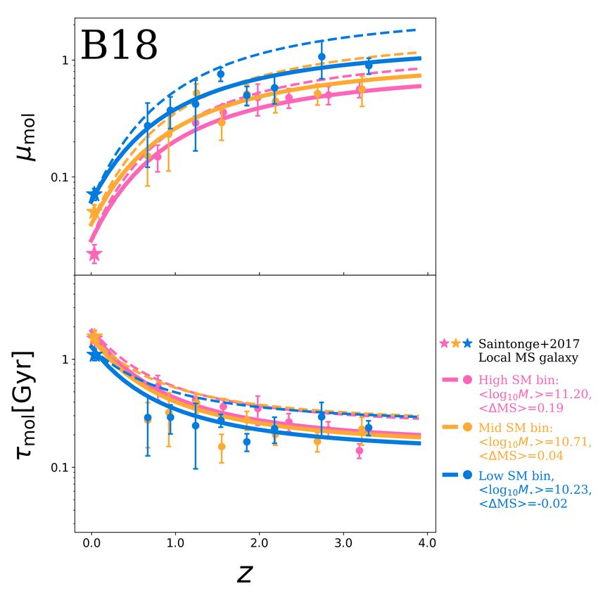
W. Tsan-Ming et al.: Molecular gas mass and extent of main-sequence galaxies across cosmic time

in the COSMOS field (A3 COSMOS) project (Liu et al. 2019a).            et al. 2009), ultraviolet (e.g., GALEX; Zamojski et al. 2007),
This mass-complete sample of MS galaxies was then subdivided           optical (e.g., Koekemoer et al. 2007; Taniguchi et al. 2007), in-
into several redshift and stellar mass bins, and a measurement         frared (e.g., Spitzer; Sanders et al. 2007), to radio wavelengths
of their mean molecular gas mass and size was performed using          (e.g., VLA; Schinnerer et al. 2010; Smolčić et al. 2017). These
a uv-based stacking analysis of their ALMA observations. This          observations have triggered numerous spectroscopic follow-up
stacking analysis allows for accurate mean gas mass and size           studies, providing nowadays more than 10,000 spectroscopic
measurements even at low stellar masses where galaxies are too         redshifts for galaxies over this field. From all these photomet-
faint to be individually-detected by ALMA. Our results provide         ric and spectroscopic multi-wavelength coverage, Laigle et al.
for the first time robust RJ-based constraints on the mean cold        (2016) built the reference COSMOS-2015 catalog, providing
gas mass of a mass-complete sample of M? > 1010 M galaxies             the photometry, redshift (photometric or spectroscopic), stellar
up to z ∼ 3. Combined with their mean far-infrared (FIR) size          mass, and SFR of more than half a million of galaxies. From
measurements, this yields the first stringent constraint of the KS     their careful analysis, Laigle et al. (2016) classified galaxies into
relation at high-redshift.                                             quiescent and star-forming based on a standard rest-frame NUV-
    The structure of the paper is as follows: in Section 2, we         R-J selection method. The mass-completeness of their SFGs is
introduce the ALMA data used in our study and our mass-                down to stellar masses of ∼ 109.3 M at z < 1.75 and ∼ 109.9 M
complete sample of MS galaxies; in Section 3, we describe the          at z < 3.50 (see their Table 6). Here we select only SFGs above
method used to estimate the mean gas mass and size of a given          their mass-completeness limit. Moreover, to avoid contamina-
galaxy population by stacking their ALMA observations in the           tion from active galactic nuclei (AGN), we exclude from our
uv-domain; in Section 4, we present our results and discuss them       analysis all galaxies classified as AGNs based on their X-Ray
in Section 5; finally, in Section 6, we summarize our findings and     luminosity (LX ≥ 1042 erg s−1 ; Szokoly et al. 2004) using the
present our conclusions.                                               latest COSMOS X-ray catalog of Marchesi et al. (2016). After
    Throughout the paper, we assume a flat ΛCDM cosmology              the selection of SFGs and exclusion of AGNs, our parent sam-
with H0 = 67.8 km s−1 Mpc−1 , ΩM = 0.308, and ΩΛ = 0.692               ple is left with 515,465 galaxies (green contours in Fig. 1). We
(Planck Collaboration et al. 2016). All stellar masses and SFRs        note that photometric redshifts in the COSMOS-2015 catalog
are provided assuming an Chabrier (2003) initial mass function.        are highly reliable even up to the redshift limit of our study, i.e.,
                                                                       z = 3.6, with a redshift accuracy of σδz/(1+z) ∼0.028 (Laigle et al.
                                                                       2016).
2. Data                                                                     To select from this parent sample galaxies residing within
                                                                       the MS of SFGs, one needs to accurately measured their SFRs.
2.1. The A3 COSMOS dataset                                             The COSMOS-2015 catalog provides such estimates but those
The A3 COSMOS project aims at homogeneously processing                 are solely based on optical-to-near-infrared SED fits performed
(i.e., calibration, imaging and source extraction) of all ALMA         by Laigle et al. (2016). While reliable for stellar masses with
projects targeting the COSMOS field that are publicly available,       M? < 1011 M and moderately star-forming galaxies, observa-
and providing these calibrated visibilities, cleaned images, and       tions from the Herschel Space Observatory have unambiguously
value-added source catalog via a single access portal (Liu et al.      demonstrated that such measurements are inaccurate for star-
2019a). In our analysis we use the A3 COSMOS 20200310 ver-             bursting or massive SFGs, in which star formation can be heav-
sion1 , i.e., all ALMA projects publicly available over the COS-       ily dust-enshrouded (e.g., Wuyts et al. 2011; Qin et al. 2019). To
MOS field by the 10th of March 2020. This database contains            accurately measure the SFR of all galaxies in our parent sam-
80 independent ALMA projects with band-6 and/or -7 obser-              ple, we use thus the approach advocated by Wuyts et al. (2011),
vations. The interferometric calibration was performed by the          i.e., applying to each galaxy the best dust-corrected star forma-
A3 COSMOS project using the Common Astronomy Software                  tion indicator available (the so-called ladder of SFR indicator;
Applications package (CASA; McMullin et al. 2007) and the              see below for details). The SFR of galaxies for which infrared
calibration scripts provided by the ALMA observatory. During           observations were available, were obtained by combining their
this calibration step, a weight is assigned to each calibrated visi-   un-obscured and obscured SFRs, following Kennicutt (1998b)
bility and this weight is key for the accuracy of our stacking anal-   for a Chabrier (2003) initial mass function,
ysis (see Sect. 3.2). Unfortunately, the definition of these weights
changed between the CASA versions used for the ALMA cycles             SFRUV+IR [M yr−1 ] = 1.09×10⁻¹⁰ (LIR [L ]+3.3×LUV [L ]), (1)
0, 1 and 2, and those used for ALMA cycles > 3. For this rea-
son, we excluded from our analysis all cycle 0, 1, and 2 ALMA          where the rest-frame LUV at 2300Å was taken from
projects. Our final database contains 64 ALMA projects, 39 in          the COSMOS-2015 catalog, and the rest-frame LIR =
band-6 and 25 in band-7. These projects include 1893 images            L(8 − 1000 µm) was calculated from their mid/far-infrared pho-
(equivalently ALMA pointings), which contain a total of 1002           tometry2 . For galaxies with multiple far-infrared photometry in
sources with > 4.35σ (Liu et al. 2019a).                               the COSMOS-2015 catalog3 , we estimated their LIR by fitting
                                                                       their PACS and SPIRE flux densities (Lutz et al. 2011; Oliver
                                                                       et al. 2012) with the SED template library of Chary & Elbaz
2.2. Our Sample
                                                                       2
                                                                          Among the 3037 galaxies of our final sample (see below), 972 (32%)
COSMOS is a deep extragalactic blind survey of two square de-          have mid-infrared 24 µm photometry and among those 482 (16%) have
grees on the sky centered at R.A. (J2000) = 10h 00m 28.6s , Dec. =     multiple far-infrared photometry. Among the 1376 galaxies of our final
+02◦ 120 21.000 (Scoville et al. 2007). This survey has been carried   sample with stellar mass > 1010 M (those detectable by our stacking
out over 46 broad and narrow bands probing the entire electro-         analysis; see Sect. 4), 852 (62%) have mid-infrared 24 µm photometry
magnetic spectrum, from X-ray (e.g., XMM-Newton; Cappelluti            and among those 461 (33%) have multiple far-infrared photometry.
                                                                        3
                                                                          The Herschel photometry in the COSMOS-2015 catalog is based on
1
  A3 COSMOS 20200310 version: https://sites.google.com/                the 24 µm prior source extraction performed by the PEP (Lutz et al.
view/a3cosmos/data/dataset_v20200310                                   2011) and HerMES (Oliver et al. 2012) consortia.

                                                                                                                Article number, page 3 of 27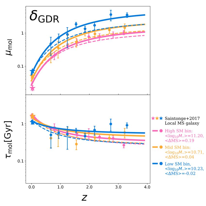
A&A proofs: manuscript no. Wang_etal_2020

Fig. 1. (Left) Stellar mass and redshift distribution in our final ALMA-covered mass-complete sample of MS galaxies (blue dots). The pink dashed
contours displays the number density of SFGs in Laigle et al. (2016), i.e., our parent sample of SFGs. The pink contour levels are in steps of 500
from 200 to 3700 galaxies per z–log10 M? bin of size 0.14 and 0.15, respectively. The orange solid line represents the stellar mass completeness limit
of SFGs in Laigle et al. (2016). The green contour shows the number density of SFGs in Laigle et al. (2016) above this stellar mass completeness
limit, i.e., our parent mass-complete sample. The green contour levels are in steps of 500 from 200 to 3700 galaxies per z–log10 M? bin of size
0.14 and 0.15, respectively. (Right) Relative ∆MS distribution in our final ALMA-covered mass-complete sample of MS galaxies (blue histogram)
and our mass-complete parent sample of SFGs (green histogram) in different stellar mass bins. In the highest stellar mass bin, the purple dashed
line shows the relative ∆MS distribution after having rejected from our final sample all ALMA primary targets, i.e., galaxies at the phase center of
the ALMA observation. The vertical blue dashed lines display the ±0.5 dex interval used to defined MS galaxies. Over this interval, the integral
of each histogram is equal to one. This normalization is needed to compare our final and mass-complete parent samples which contain 3,037 and
515,465 galaxies, respectively.

(2001). For galaxies without a multiple far-infrared photometry             among the 269 galaxies of our final sample with stellar mass
but a mid-infrared 24µm detection in the COSMOS-2015 cat-                   > 1010 M (that is, those detectable by our stacking analysis; see
alog, we estimated their LIR by scaling the MS SED template                 Sect. 4) and with SFR>100 M yr−1 , only 54 have their SFRs
of Elbaz et al. (2011) to their 24µm flux densities (Le Floc’h              solely based on their SED fits and thus potentially underesti-
et al. 2009). This particular MS SED template was chosen be-                mated by ∼ 0.3−0.5 dex (see Fig. 2). Finally, we note that at high
cause it provides accurate 24µm-to-LIR conversions over the red-            SFRs, where a high fraction of galaxies are individually-detected
shift and stellar mass ranges probed in our study (Elbaz et al.             by ALMA, our SFRs agree with those from the A3 COSMOS
2011). For galaxies without any mid- and far-infrared photom-               catalog, i.e., inferred with MAGPHYS (da Cunha et al. 2008,
etry, we used the SFRs measured by Laigle et al. (2016) and                 2015) SED fitting combining the COSMOS-2015 photometry
which were obtained by fitting their optical-to-near-infrared pho-          with super-deblended Herschel (Jin et al. 2018) and ALMA pho-
tometry with the Bruzual & Charlot (2003) SED model. We                     tometry.
verified that towards intermediate SFRs, i.e., where the frac-
tion of galaxies with a mid/far-infrared detection starts to de-
crease (i.e., 0 < log(SFRIR+UV ) < 1.5), our (UV+IR)-based SFR
measurements agree with those solely based on this optical-to-
near-infrared SED fits, with a median log(SFRIR+UV /SFRSED ) of                 From their redshift, stellar mass, and SFR, we can measure
0.09+0.39                                                                   the offset of each of these galaxies from the MS, i.e., ∆MS =
     −0.53 (Fig. 2). This agreement ensures a smooth transition be-         log(SFR(z, SM)/SFRMS (z, SM)). To this end, we used the main-
tween the different steps of our ladder of SFR indicators. Also,
                                                                            sequence calibration of Leslie et al. (2020), as it is also based on
Article number, page 4 of 27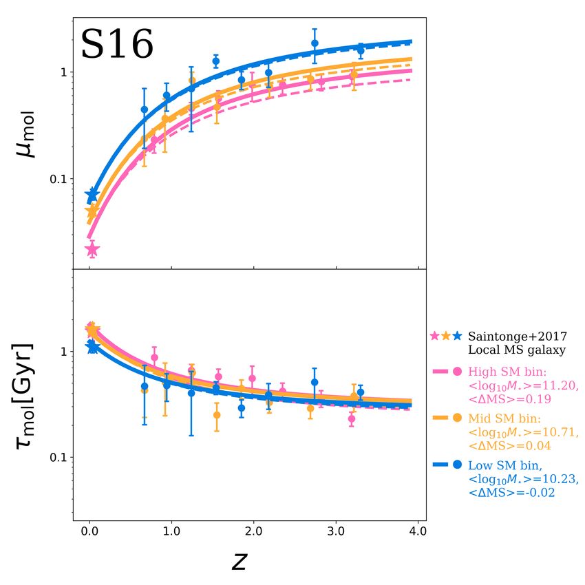
W. Tsan-Ming et al.: Molecular gas mass and extent of main-sequence galaxies across cosmic time
The ALMA archive cannot be treated as a real blind survey
and thus our ALMA coverage selection criteria could have in-
troduced a bias in our final ALMA-covered mass-complete MS
galaxy sample. As an example (though rather unrealistic), if all
ALMA projects in COSMOS would have targeted MS galaxies
with ∆MS= 0.3 dex, our final sample would naturally be biased
toward this population and thus not be representative of the entire
MS galaxy population. A simple way to test the presence of such
bias is to compare the ∆MS distributions of our final and par-
ent samples for different stellar mass bins (Fig. 1; right panels).
As expected, our parent sample (green histogram) exhibits in all
stellar mass bins a Gaussian distribution centered at 0 and with a
0.3 dex dispersion. At low stellar masses (M? < 1010.0 M ), our
final sample follows the same distribution, with a Kolmogorov-
Smirvov 99% probability of being drawn from the same sample
(this finding remaining true even if we divide further these stellar
mass bins into several redshift bins). Indeed, in these low stellar
mass bins, only 5% of our galaxies are located at the phase cen-
ter of the ALMA image and thus were the primary target of the
ALMA observations. In the highest stellar mass bins, we note,
Fig. 2. Comparison of the SFRs obtained from the COSMOS-2015 cat- however, that the ∆MS distribution of our final sample is signif-
alog, i.e., SFRSED , to the SFRs obtained from the ladder of SFR, i.e., icantly skewed towards high ∆MS values (this finding remain-
SFRUV+IR . Number densities are displayed in log-scale. Blue circles rep- ing again true if we divide further these stellar mass bins into
resent the median value of log(SFRSED ) in log(SFRUV+IR ) bins, starting several redshift bins). In these stellar mass bins, about 63% of
from -0.25 dex and with a bin size of 0.5 dex. Error bars correspond to our galaxies are the primary targets of the ALMA observations
the 16th and 84th percentiles. The pink line is the one-to-one relation. (i.e., located at the phase center), and thus potentially affected
by complex and uncontrollable selection biases. Excluding these
primary targets from our galaxy sample yields ∆MS distribution
the mass-complete COSMOS-2015 catalog: in much better agreement with those of our parent sample. In the
0
10 Mt rest of our analysis, at high masses, we will show our stacking
log(SFRMS (z, SM)) = S 0 − a1 t − log 1 + M ,
results before and after excluding these primary-target galaxies.
10 (2) In addition, we will account for these ∆MS distributions while
0
Mt = M0 − a2 t, fitting the cosmic and stellar mass evolution of the mean molec-
ular gas content of MS galaxies.
where M is log(M? /M ), t is the age of the universe in Gyr,
S 0 =2.97, M0 =11.06, a1 =0.22, and a2 =0.12. Our mass-complete
sample of MS galaxies was then constructed by selecting galax- 3. Method
ies with ∆MS between −0.5 and 0.5 (e.g., Rodighiero et al.
2014). This sample contains 92,739 galaxies. ALMA has revolutionized the study of high-redshift SFGs at
Finally, from this mass-complete sample of MS galaxies, (sub)millimeter wavelengths. Nevertheless, even with its un-
we selected those with an ALMA band-6 (∼ 243 GHz) or parallel sensitivity, ALMA cannot detect within a reasonable
band-7 (∼ 324 GHz) coverage in the A3 COSMOS database observing time MS galaxies with M? < 1010.5 M at z > 0.5.
(see Sect. 2.1). Here, we only consider galaxies well within the Consequently, despite including all individually-detected galax-
ALMA primary beam, i.e., where the primary beam response is ies within the A3 COSMOS images (i.e., primary targets and
higher than 0.5. This conservative primary beam cut was used serendipitous detections), the final sample of Liu et al. (2019b)
because uncertainties in the primary beam response far from the is still mostly restricted to the high-mass end of the SFG popu-
phase center can significantly affect our stacking analysis (see lation. The emission of such low-mass high-redshift SFGs cap-
Sect. 3.2). In addition, to avoid contamination by bright neigh- tured within these images is too faint to be individually-detected,
bouring sources, we excluded from our analysis galaxy pairs and thus remains unexploited. To statistically retrieve the faint
(< 200. 0) with S ALMA
1
/S ALMA
2
> 2 or M?1 /M?2 > 3 (for ALMA emission of this SFG population, we need to perform a stack-
undetected galaxies, assuming a first-order Mgas − M? corre- ing analysis. As already mentioned, stacking over the entire
lation). About 8% of our galaxies are excluded by these crite- A3 COSMOS dataset presents two challenges when compared to
ria. However, we note that most of these excluded galaxy pairs standard stacking analysis performed with Spitzer, Herschel, or
(∼ 95%) are due to projection effects (∆z > 0.05). This implies individual ALMA projects. Indeed, the A3 COSMOS database is
that the exclusion of these galaxies does not introduce any bi- heterogeneous in terms of observed frequencies and spatial res-
ases into our final ALMA-covered mass-complete sample of MS olution. The frequency-heterogeneity problem is simply solved
galaxies. There are 3,037 galaxies in this final sample. The left by a prior re-scaling of each individual dataset to a common rest-
panel of Fig. 1 shows the stellar mass and redshift distribution frame luminosity frequency using locally calibrated submillime-
of our parent and final samples. Our final sample probes a broad ter SEDs (Sect. 3.1), while the spatial resolution-heterogeneity
range in redshifts and stellar masses, similar to that probed by problem is solved by performing our stacking analysis in the uv-
our parent sample. We verified that our parent and final samples domain (Sect. 3.2).
have consistent stellar mass, redshift and LIR distributions, with In the following, we describe in detail the different steps of
Kolmogorov-Smirvov probabilities of 99%, 99%, and 96% of our stacking analysis, while the validation of this methodology
being drawn from the same distribution, respectively. via Monte Carlo simulations is presented in Appendix A.
Article number, page 5 of 27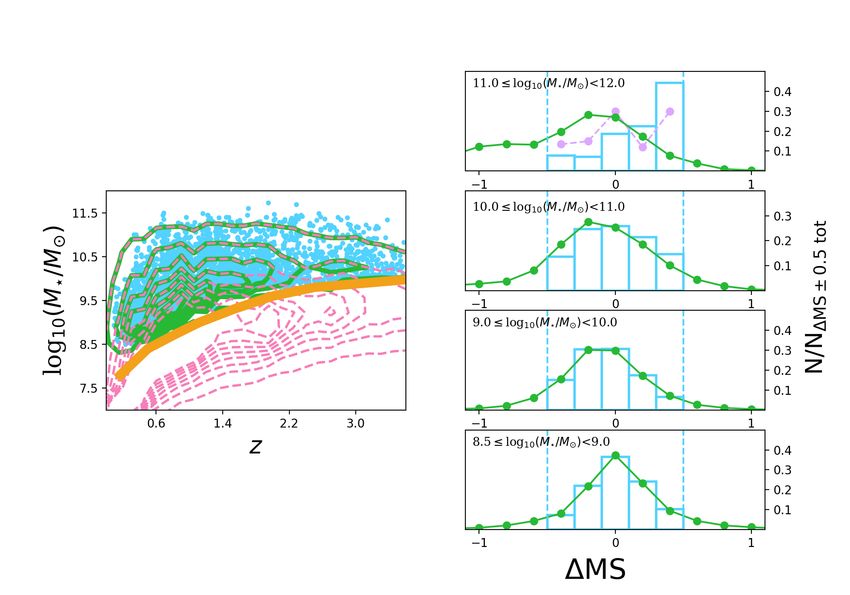
A&A proofs: manuscript no. Wang_etal_2020

3.1. From observed-frame flux densities to rest-frame                              the original weights of all visibilities (i.e., those accounting for
     luminosities                                                                  their system temperature, channel width, integration time. . . )
                                                                                   were properly re-normalized and could thus be used for the
The A3 COSMOS observations were performed at different fre-                        forthcoming uv-model fit and image processing.
quencies and the galaxies to be stacked also lie at slightly dif-                       To measure the stacked rest-frame 850 µm luminosity of
ferent redshifts. Therefore, prior to proceeding with our stack-                   each of our stellar mass–redshift bins, i.e., L850 stack
                                                                                                                                            , we used two
ing analysis, we needed to convert the ALMA observations of a                      different approaches. First, we extracted this information from
given galaxy from observed flux density to its rest-frame lumi-                    the uv-domain by fitting a single component model to the stacked
nosity at 850 µm, i.e., L850
                         rest
                              . To do so, we used the MS SED tem-                  measurement set. This fit was performed using the CASA task
plates of Béthermin et al. (2012), which accurately capture the                    uvmodelfit, assuming a single Gaussian component and fixing
monotonic increase of the dust temperature of MS galaxies with                     its position to the stacked phase center. Second, we measured
redshift (e.g., Magdis et al. 2012; Magnelli et al. 2014). First,                    stack
                                                                                   L850    from the image-domain. To do so, we imaged the stacked
we computed the SED template luminosity ratio at rest-frame                        measurement set with the CASA task tclean, using Briggs nat-
850 µm and the observed rest-frame wavelength of the galaxy of                     ural weighting and cleaning the image down to 3σ. Then, we fit-
interest,                                                                          ted a 2D Gaussian model to the cleaned image using the Python
ΓSED = L850
        SED
            / LλSED         .                                                (3)   Blob Detector and Source Finder package (PyBDSF; Mohan &
                 obs /(1+z)                                                        Rafferty 2015). For all our stellar mass–redshift bins, these two
The observed ALMA visibility amplitudes toward this galaxy,                        approaches agreed within the uncertainties.
i.e., | V(u, v, w) |λobs , – which are in units of flux density – were                  Our uv-domain and image-domain fits provide us also with
then converted into rest-frame 850 µm luminosity following:                        the mean size (or upper limit) of the galaxy population in a
                                                                                   given stellar mass–redshift bin. From the intrinsic (i.e., beam-
            850 = 4 π DL × | V(u, v, w) |λobs × Γ
|L(u, v, w)|rest                                     / (1 + z),
                       2                         SED
                                                                             (4)   deconvolved) full width at half maximum (FWHM) of the ma-
                                                                                   jor axis outputted by uvmodelfit or PyBDSF, we define the
where DL is the luminosity distance of the galaxy of interest.                     effective –equivalently half-light– radius (Reff ) of the stacked
This re-scaling of the amplitude (and weights) of the ALMA vis-                    population following Jiménez-Andrade et al. (2019), i.e., Reff ≈
ibilities was performed for each stacked galaxy using the CASA                     FWHM/2.43. Then, we express these mean size measurements
tasks gencal and applycal.                                                         in form of circularized radii, Rcirc
                                                                                                                      eff ,
                                                                                                    r
                                                                                                       b
3.2. Stacking in the uv-domain                                                       eff = Reff ×
                                                                                   Rcirc                 ,                                             (6)
                                                                                                       a
Stacking in the uv-domain relies on the exact same principle as                    where b/a is the axis ratio measured with uvmodelfit or
aperture synthesis. The only difference is that one combines mul-                  PyBDSF.
tiple baselines pointing at the same galaxy population instead of                       Finally, to infer the uncertainties associated to these stacked
multiple baselines pointing at the same galaxy. The tools or tasks                 rest-frame 850 µm luminosity and size measurements, we used
needed to perform stacking in the uv-domain are thus all readily                   a standard re-sampling method. These uncertainties account not
available in CASA. For each of our stellar mass-redshift bin and                   only for the instrumental noise in the stacked measurement set
each galaxy within these bins, we proceeded as follow. First, we                   (i.e., the detection significance) but also for the intrinsic distribu-
time- and frequency-average their measurement set, producing                       tion of L850 and size within the stacked galaxy population. For a
one averaged visibility per ALMA scan (lasting typically 30s                       stellar mass–redshift bin containing N galaxies, we performed
and originally divided into 10 × 3s integration) and ALMA spec-                    N different realizations of our stacking analysis, removing in
tral window (probing typically 2 GHz and originally divided into                   each realization one galaxy of the stacked sample. The uncer-
                                                                                                 stack
100s of channels). This step, which was performed using the                        tainties on L850    and size are then given by the standard deviation
CASA task split, is crucial to keep the volume of our final                        of these
                                                                                         √    quantities   measured over these realizations multiplied
stacked measurement sets within current computing capabilities.                    by N. We note that because there is a possible mismatch of
These averaged visibilities were then re-scaled from observed-                     ∼ 000. 2 between the stacked optical-based position and the actual
frame flux density into rest-frame 850 µm luminosity using the                     (sub)millimeter position of the sources (e.g., Elbaz et al. 2018),
CASA tasks gencal and applycal (see Sect. 3.1). Finally, the                       the average FIR sizes inferred in our study could be slightly over-
phase center of these averaged and re-scaled visibilities were                     estimated. This is further discussed in Sect. 4.3.
shifted to the coordinate of the stacked galaxy. This step was                          Note that although some studies have used median stacking
performed using the CASA package STACKER (Lindroos et al.                          to mitigate the contribution of bright outliers to the stacked flux
2015) following,                                                                   densities (e.g., Algera et al. 2020; Feltre et al. 2020; Fudamoto
                                                                                   et al. 2020; Gabányi et al. 2021; Johnston et al. 2021), we de-
                                            1        2π
                  850 = L(u, v, w)850
Lshifted (u, v, w)rest                              e λ iB·(Ŝ 0 −Ŝ k )
                                  rest                                             cided to perform our analysis using a mean stack, i.e., in the uv-
                                                                             (5)
                                         AN (Ŝ k )                                domain, our models are fitted to the weighted mean visibility am-
                                                                                   plitudes and our images are created by tclean using weighted
where L(u, v, w)rest 850 is the averaged and re-scaled visibility, Ŝ 0 is         mean visibilities. This choice was made for the following rea-
a unit vector pointing to the original phase center, Ŝ k is a unit                sons: (i) the impact of bright outliers is already mitigated by our
vector pointing to the position of the stacked galaxy, AN (Ŝ k )                  −0.5 < ∆MS< 0.5 selection, which by construction excludes
is the primary beam attenuation in the direction Ŝ k , B is the                   gas-rich starbursts; (ii) the impact of bright outliers is accounted
baseline of the visibility. The final stacked measurement set                      for in our uncertainties (i.e., re-sampling method); and finally
of a given stellar mass-redshift bin was then obtained by con-                     (iii) Schreiber et al. (2015) and Leslie et al. (2020), which thor-
catenating the shifted, re-scaled and averaged visibilities, i.e.,                 oughly tested mean and median stacking, concluded both that
Lshifted (u, v, w)rest
                  850 , of all galaxies within this bin using the CASA             median stacking is biased toward higher values at low S/N be-
task concat. Because all these steps were performed in CASA,                       cause the median is not a linear operation and that the stacked
Article number, page 6 of 27
W. Tsan-Ming et al.: Molecular gas mass and extent of main-sequence galaxies across cosmic time
distribution is intrinsically a log-normal distribution skewed to- galaxy populations are thus detected and spatially resolved by
ward bright sources. As a result, median stacked fluxes are dif- our stacking analysis. In the image-domain, this translates into
ficult to interpret and are often not measuring the median nor bright spatially-resolved phase-center emission – i.e., with a me-
mean fluxes, but something in between. We note, however, that dian synthesised beam FWHM of 000. 5 and an median angular
the median visibility amplitudes of each of our stacked bins are size-to-synthesised beam FWHM ratio of 1.5 – that are well de-
consistent, within the uncertainties, with the mean visibility am- scribed by single 2D Gaussian components. In our intermediate
plitudes (see open symbols in Fig. 3). stellar mass bin (i.e., 1010.5 ≤ M? /M < 1011.0 ), the number
of stacked sources per redshift bin increases (43–81), while the
fraction of them being individually detected decreases to about
3.3. From rest-frame 850 µm luminosities to molecular gas
10%. As for our highest stellar mass bin, our stacking analysis
masses
yields high significance detections (i.e., S/Npeak > 5) in all of
The literature contains a plethora of relations linking molecu- our redshift bins and those are spatially resolved at our median
lar gas mass of galaxies with their (sub)millimeter luminosi- synthesised beam FWHM of 000. 6. Finally, in our lowest stellar
ties (e.g., Bourne et al. 2013; Groves et al. 2015; Scoville et mass bin (i.e., 1010 ≤ M? /M < 1010.5 ), the number of stacked
al. 2017; Bertemes et al. 2018; Saintonge et al. 2018; Kaasi- sources per redshift bin increases even further (79–131) and only
nen et al. 2019). All of them rely on an assumed gas-to-dust few of them are individually detected (1%). In this low stellar
mass ratio (or a direct 870 µm luminosity-to-gas mass ratio) mass bin, the same patterns are observed, i.e., spatially-resolved
that might or might not depend on the metallicity. Liu et al. detections in the uv- and image-domain (with a median synthe-
(2019b) thoroughly studied how these different relations influ- size beam FWHM of 000. 7), though at lower significance, i.e.,
ence our molecular gas mass estimation, using a sample of galax- 3 < S/Npeak < 9. This implies that the number of stacked galax-
ies down to a stellar mass of ∼ 1010.3 M . They found that ies (controlled by the stellar mass function of MS galaxies) does
metallicity-dependent relations (Rémy-Ruyer et al. 2014; Gen- not increase sufficiently to fully counter-balance the decrease
zel et al. 2015) and the 850 µm luminosity-dependent relation of their molecular gas content with respect to the most mas-
of Hughes et al. (2017) only differ by ∼0.15–0.25 dex (which sive population. Nevertheless, even in this low stellar mass bin,
is comparable to the observed scatter), and that the relation of our stacking analysis yields clear detection (S/Npeak > 3), espe-
Hughes et al. (2017) provided the best agreement with local ob- cially when considering both the uv-domain and image-domain
servations (e.g., Bertemes et al. 2018; Saintonge et al. 2018). constraints. We note that pushing this stacking analysis to lower
They concluded that the 850 µm luminosity-dependent relation stellar masses (M? < 1010 ) did not produce any significant de-
is thus the most preferable relation for galaxies down to a stel- tection. These results are thus not presented here and not dis-
lar mass of M? ∼ 1010.3 M and for which no metallicity mea- cussed further in the paper.
surements are available. Based on their analysis, we decided to We conclude that our stacking analysis provides robust mean
use this empirically-calibrated relation of Hughes et al. (2017). molecular gas mass and FIR size measurements for M? >
The mean molecular gas mass of a given galaxy population (i.e., 1010 M MS galaxies from z ∼ 0.4 to 3.6. Considering that in
Mmol ) is thus computed from their stacked rest-frame 850 µm lu- our highest and lowest stellar mass bins only 37% and ∼ 1%
minosities following, of these galaxies were individually detected in the A3 COSMOS
catalog, respectively, our stacking analysis clearly provides the
log10 Mmol = (0.93 ± 0.01) · log10 L850 − (17.74 ± 0.05), (7) first unbiased ALMA view on the gas content and size of MS
galaxies.
where Mmol already includes the 1.36 correction factor to ac-
count for helium and assumes a CO-to-Mmol conversion factor
(i.e., αCO ) of 6.5 (K km s−1 pc2 )−1 . 4.1. The molecular gas content of MS galaxies
In Section 4.5.1 and Appendix B, we thoroughly present and The redshift evolution of the molecular gas mass of MS galax-
discuss the impact on our results of using different gas mass cal- ies inferred from our stacking analysis is shown in Fig. 4. It is
ibration relations. In brief, the main conclusions of our paper compared to analytical predictions from the literature (Scoville
are not qualitatively affected by this particular choice; the H17 et al. 2017; Liu et al. 2019b; Tacconi et al. 2020), individually-
method yields measurements which are bracket by those inferred detected MS galaxies taken from the A3 COSMOS catalog (Liu
from other relations; and, finally, measurements obtained using et al. 2019b) and a local reference (i.e., z ∼ 0.03) taken from
H17 are in good agreement with Tacconi et al. (2020) at high Saintonge et al. (2017). In addition, in Fig. 6, we present the evo-
stellar masses, i.e., where this latter study can be considered as lution of the molecular gas fraction (i.e., µmol = hMmol i/hM? i)
the reference. of MS galaxies as a function of redshifts and stellar masses. We
note that for our galaxies in common with the A3 COSMOS cata-
4. Results log, the stellar masses used here (i.e., those from the COSMOS-
2015 catalog) are about 0.22 dex lower than those reported in
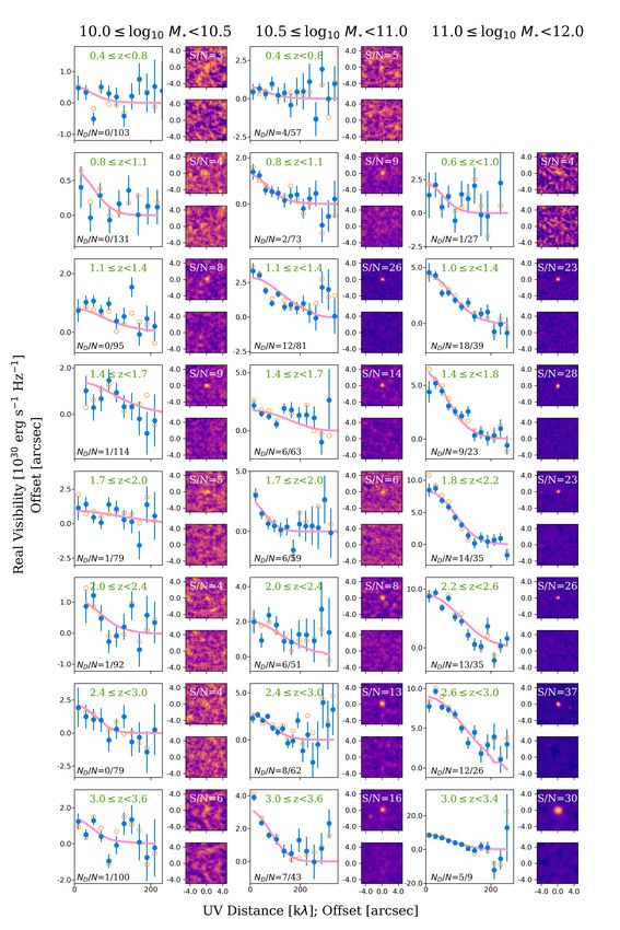
The results of our stacking analysis are shown in Fig. 3 and the A3 COSMOS catalog. This offset, which is also discussed
summarized in Tab. 1. In our highest stellar mass bin (i.e., in Liu et al. (2019b), is likely explained by the fact that stellar
1011 ≤ M? /M < 1012 ; right-most column), the number of masses in the A3 COSMOS catalog rely on full optical-to-mm
stacked sources per redshift bin varies from 9 to 39, with about energy-balanced SED fits performed with MAGPHYS. While this
37% of them being individually detected. In this stellar mass bin, offset is observed for massive galaxies, it might not be present
our stacking analysis yields high significance detections, with at . 1010.5 M , where the number of galaxies available in the
peak signal-to-noise ratios (S/Npeak ) greater than 20, except in A3 COSMOS catalog is too scarce to provide meaningful com-
our lowest redshift bin with S/Npeak ∼ 4. In the uv-domain, those parison with the COSMOS-2015 catalog. In any case, when
high significance detections are characterized by a Gaussian- comparing our analytical predictions to those from Liu et al.
like decrease of the stacked visibility amplitudes with the uv- (2019b), we thus show both their original predictions and those
distance, well fitted by our single component model. These inferred by accounting for this systematic 0.22 dex offset.
Article number, page 7 of 27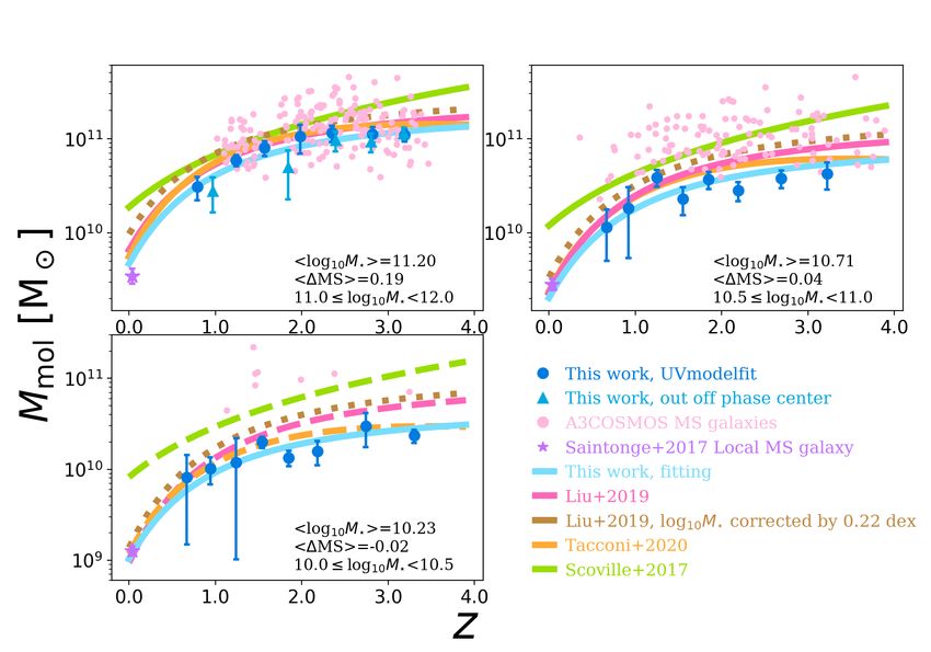
A&A proofs: manuscript no. Wang_etal_2020

Fig. 3. Results of our stacking analysis for MS galaxies in the uv- and image-domain. For each stellar mass–redshift bin, the left panel shows the
single component model (pink solid line) fitted to the (stacked) mean visibility amplitudes (blue filled circles) using the CASA task uvmodelfit.
Open orange circles show the median visibility amplitudes, which are consistent, within the uncertainties, with the mean visibility amplitudes. The
top-right and bottom-right panels show, respectively, the stacked and residual images, the latter being obtained by subtracting from the former the
single 2D Gaussian component fitted by PyBDSF. The number of individually detected galaxies (ND ) and the number of stacked galaxies (N) in
each stellar mass–redshift bin is reported in the left panel (i.e., ND /N) , while the detection significance, i.e., S/Npeak , is reported in the upper right
panel.
Article number, page 8 of 27

Table 1. Molecular gas mass and size properties of main-sequence galaxies.
                                                                                                                                                                                                                circ    circ      circ
                                          M?                   z          N     ND     hzi        hM? i         hSFRi          h∆MSi      hνobs i       hL850−uv i      S/Npeak     Mmol−uv       Mmol−py      θbeam   θmol−uv   θmol−py                                                                                                 Rcirc
                                                                                                                                                                                                                                                                                                                                           eff−uv
                                                                                               log10 [M ]   log10 [M yr−1 ]               GHz       1030 erg s−1 Hz−1             log10 [M ]    log10 [M ]    arcsec   arcsec    arcsec                                                                                                   kpc
                                         (1)                  (2)        (3)    (4)     (5)        (6)             (7)           (8)       (9)            (10)           (11)         (12)         (13)        (14)     (15)      (16)                                                                                                    (17)
                                11.0≤ log10 M?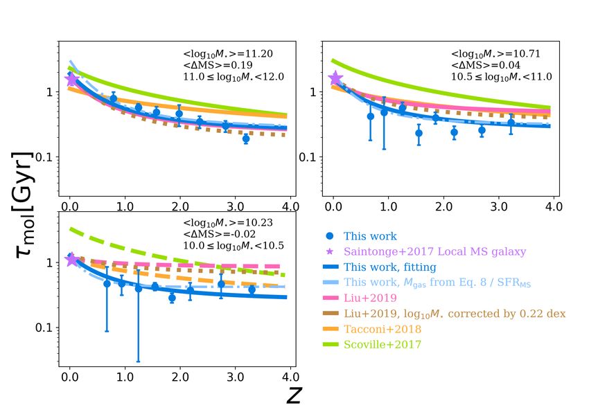
A&A proofs: manuscript no. Wang_etal_2020

Fig. 4. Redshift evolution of the mean molecular gas mass of MS galaxies in three stellar mass bins, i.e., 1011 ≤ M? /M < 1012 , 1010.5 ≤
M? /M < 1011 , and 1010 ≤ M? /M < 1010.5 . Blue circles show our uv-domain measurements, while in the highest stellar mass bin blue triangles
show those obtained after excluding ALMA primary-target galaxies from our stacked sample (see Sect. 2.2). Pink circles are individually-detected
MS galaxies taken from the A3 COSMOS catalog (Liu et al. 2019b), while purple stars present the local reference taken from Saintonge et al.
(2017). Lines show the analytical evolution of the gas fraction as inferred from our work (blue lines), from Scoville et al. (2017, green line), from
Liu et al. (2019b, pink line), from Tacconi et al. (2020, orange), and finally, from Liu et al. (2019b, brown dotted line) but this time accounting
for the systematic 0.22 dex offset observed between their and our stellar mass estimates. In our lower stellar mass bin, lines from the literature are
dashed as they mostly rely on extrapolations. Note that here and in all following figures, the values of hM? i and h∆MSi given in each panels are
simply used to plot the analytical evolution of the gas fraction. These values naturally vary for each stacked measurements and is accounted for
by our MCMC analysis. This avoids averaging biases that could arise if one would simply fit our stacked measurements using htcosmic i, hM? i, and
h∆MSi.

    Our measurements reveal a significant evolution of the                  where tcosmic is the cosmic time in units of Gyr, and M? is
molecular gas mass of MS galaxies with both redshifts and stel-             in units of M . Because our analysis does not probe a large
lar masses. For all stellar mass bins, the molecular gas masses             dynamic range in ∆MS, we fixed a and ak to the values re-
of MS galaxies (equivalently molecular gas fraction) increase by            ported by Liu et al. (2019b), i.e., a = 0.4195 and ak =
a factor of ∼24 from z ∼ 0 to z ∼ 3.2. In addition, at a given              0.1195, respectively. To constrain the remaining parameters of
redshift, the molecular gas masses of MS galaxies significantly             Eq. 8, we then performed a standard Bayesian analysis using the
increase with stellar masses. This trend is, however, sub-linear in         python Markov Chain Monte Carlo (MCMC) package emcee
the log-log space, which implies that the molecular gas fraction            (Foreman-Mackey et al. 2013). In this analysis, we accounted
of MS galaxies decreases with stellar mass at a given redshift              for the redshift, stellar mass, and ∆MS of each galaxy in a
(Fig. 6). To obtain a more quantitative constraint on the stellar           given stacked bin, i.e., in each MCMC step, we compared our
mass and redshift dependencies of evolution of the molecular gas            stacked measurements, hMgas      i               i
                                                                                                                i, to h f ( tcosmic , M?i , ∆MSi )i and
fraction of MS galaxies, we fitted our measurements, together                        i
                                                                            not f (htcosmic                i
                                                                                            i, hM?i i, h∆MS i), where i is the ith galaxy of our
with the local reference, following Liu et al. (2019b), i.e.,               stacked bin and f is the fitted function. This avoids averag-
log10 µmol = (a + ak × log10 (M? /1010 )) × ∆MS                             ing biases that could arise if one would simply fit our stacked
                                                                            measurements using htcosmic i
                                                                                                           i, hM?i i, and h∆MSi i. Results of this
           + b × log10 (M? /1010 )                                          MCMC analysis are shown in Fig. 5, with b = −0.468−0.070               +0.070
                                                                                                                                                          ,
                                                                      (8)
           + (c + ck × log10 (M? /1010 )) × tcosmic                                      +0.008                +0.059                       +0.011
                                                                            c = −0.122−0.008 , d = 0.572−0.060 , and ck = 0.002−0.011 . These
           + d,                                                             results unambiguously demonstrate that the molecular gas frac-

Article number, page 10 of 27
W. Tsan-Ming et al.: Molecular gas mass and extent of main-sequence galaxies across cosmic time
By comparing our results with those from the A3 COSMOS
catalog, one immediately notices that these individually-detected
galaxies systematically lie above our measurements. This sys-
tematic offset results from an observational bias. First of all, at a
given redshift and stellar mass, the A3 COSMOS catalog mostly
contains galaxies on the upper part of the MS because those
galaxies have higher molecular gas mass (a > 0 in Eq. 8) and are
thus more likely to be individually detected. This observational
bias was, however, accounted for when fitting the A3 COSMOS
population using Eq. 8. This ‘correction’ can be seen in Fig. 4
by noticing that the A3 COSMOS analytical predictions for MS
galaxies systematically lies below the A3 COSMOS data-points.
Nevertheless, at a given redshift, stellar mass, and ∆MS, the
A3 COSMOS catalog could still be biased toward galaxies with
a bright millimeter emission and thus high molecular gas mass
(see discussion in Liu et al. 2019b). Our measurements, which
are not affected by this bias and which lie systematically below
those of Scoville et al. (2017), Liu et al. (2019b), and Tacconi
et al. (2020), clearly demonstrate the presence of this residual
observational bias in these literature studies. By averaging at a
given redshift and stellar mass all MS galaxies in the field, our
stacking analysis reveals their true mean molecular gas mass.
Taken at face value, our findings imply that previous studies
might have systematically overestimated by at least 10−40% the
Fig. 5. Probability distributions of the parameters in Eq. 8, as found by gas content of MS galaxies in redshift and stellar mass bins with
fitting our stacked measurements using a MCMC analysis. The dashed relatively high detection fraction (i.e., mostly M? > 1011 M ),
vertical lines show the 16th, 50th, and 84th percentiles of each distribu-
and by 10 − 60% in bins with low detection fraction. While
tion.
significant, one should, however, acknowledge that these offsets
remain reasonable considering all the selection biases affecting
these previous studies. The impact of this finding for galaxy evo-
lution models is discussed in Sect. 5.
4.2. The molecular gas depletion time of MS galaxies
The redshift evolution of the molecular gas depletion time (i.e.,
τmol = Mmol /SFR) of MS galaxies as inferred from our stacking
analysis is shown in Fig. 7, together with analytical predictions
from Scoville et al. (2017), Liu et al. (2019b), and Tacconi et
al. (2020) as well as the local reference for MS galaxies taken
from Saintonge et al. (2017). Again, to obtain a more quantita-
tive constraint on the stellar mass and redshift dependencies of
the molecular gas depletion time of MS galaxies, we fitted our
measurements, together with the local reference, following Liu
et al. (2019b), i.e.,
log10 τmol = (a + ak × log10 (M? /1010 )) × ∆MS
Fig. 6. Redshift evolution of the mean molecular gas fraction of MS
+ b × log10 (M? /1010 )
galaxies. Circles show the mean molecular gas fraction from our work. (9)
Stars present the local reference taken from Saintonge et al. (2017). + (c + ck × log10 (M? /1010 )) × tcosmic
Lines display the analytical evolution of the molecular gas fraction
+ d.
inferred from our work. Symbols and lines are color-coded by stel-
lar mass, i.e., pink for 1011 ≤ M? /M < 1012 , orange for 1010.5 ≤
Our analysis does not probe a large dynamic range in ∆MS, we
M? /M < 1011 , and blue for 1010 ≤ M? /M < 1010.5 .
thus fixed a and ak to the values reported by Liu et al. (2019b),
i.e., a = −0.5724 and ak = 0.1120. Results of our MCMC anal-
ysis are shown in Fig. 8, with b = 0.055+0.069 +0.008
−0.071 , c = 0.049−0.008 ,
tion of MS galaxies decreases with stellar masses (i.e., b < 0) +0.056 +0.010
d = −0.643−0.057 , and ck = 0.016−0.010 . Because the depletion
while it increases with redshifts (i.e., c < 0; see blue solid lines time is the ratio of Mmol by SFR, we also display in Fig. 7 the
in Fig. 4). Note that repeating this MCMC analysis while fix- redshift evolution of depletion time as one would infer by di-
ing a = 0 and ak = 0 (i.e., considering that our measurements viding Mgas (z, M∗ , ∆MS) from Eq. 8 by the SFRMS (z, M∗ , ∆MS)
are for ∆MS = 0 galaxies), the likelihood of our fit decreases from Leslie et al. (2020, dash-dotted light-blue line). Finally, in
but the inferred gas fraction evolution remains qualitatively con- Fig. 9, we compare the redshift evolution of the molecular gas
sistent with our previous fit albeit with a somewhat flatter stel- depletion time as inferred for our three stellar mass bins.
lar mass dependency, i.e., b = −0.252+0.072 +0.008
−0.072 , c = −0.114−0.008 , In all our stellar mass bins, the molecular gas depletion time
+0.061 +0.011
d = 0.481−0.061 , and ck = −0.016−0.011 . of MS galaxies decreases by a factor of ∼ 3 − 4 from z ∼ 0
Article number, page 11 of 27A&A proofs: manuscript no. Wang_etal_2020 Fig. 7. The redshift evolution of molecular gas depletion time of MS galaxies in three stellar mass bins, i.e., 1011 ≤ M? /M < 1012 , 1010.5 ≤ M? /M < 1011 , and 1010 ≤ M? /M < 1010.5 . Blue circles show our uv-domain molecular gas mass measurements divided by the mean SFR of each of these stacked samples. Purple stars show the local MS reference taken from Saintonge et al. (2017). Lines present the analytical evolution of the molecular gas depletion time as inferred from our work (blue lines; see text for details), from Liu et al. (2019b, pink line), from Scoville et al. (2017, green line), and from Tacconi et al. (2020, orange line). In our lower stellar mass bin, lines from the literature are dashed as they mostly rely on extrapolations. to z ∼ 3.2, with, however, most of this decrease happening at attributed to a miss-match in SFRMS (z, M∗ , ∆MS), i.e., at a given z . 1.0. At z & 1, the molecular gas depletion time of MS galax- stellar mass, the mean SFR of z ∼ 0 MS galaxies as predicted by ies remains instead roughly constant with redshifts and stellar Leslie et al. (2020) does not match that observed by Saintonge masses with a value of ∼ 300 − 500 Myr. While such evolution is et al. (2017). This disagreement is, however, not unexpected as qualitatively predicted by all literature studies, its amplitude as the sample used in Leslie et al. (2020) was restricted to z > 0.3 well as its exact redshift- and stellar mass-dependencies quan- galaxies. titatively disagree (see Fig. 7). For example, our measurements and those from Liu et al. (2019b) agree at high stellar masses, In general, we conclude that our depletion times agree at high but differ by ∼ 30 − 40% in our lower stellar mass bins. These stellar masses with Liu et al. (2019b), i.e., where their study differences are likely explained by the observational biased dis- relies on a large and robust amount of ALMA-based measure- cussed in Sect. 4.1 which implies that the mean molecular gas ments of MS galaxies; while our depletion time agree better at mass and thus depletion time of MS galaxies inferred by Liu et low stellar masses with Tacconi et al. (2020), i.e., where their al. (2019b) are slightly overestimated especially at low stellar study, contrary to that of Liu et al. (2019b), still relies on some masses. The same effect likely explains the ∼ 20 − 30% overesti- observational measurements of MS galaxies thanks to their Her- mation of the molecular gas depletion time inferred in Tacconi et schel stacking analysis. Like our measurements, those from Tac- al. (2020) in most redshift–stellar mass bins probed here. While coni et al. (2020) predict only a minor evolution of the molecu- our direct analytical fit of the redshift/stellar mass evolution of lar gas depletion time of MS galaxies with stellar masses. This the molecular gas depletion time (solid blue lines in Fig. 7) implies that the flattening of the MS at high stellar masses ob- matches relatively well the local reference from Saintonge et al. served in most studies (i.e., log10 SFRMS = 0.7× log10 M?MS + C) (2017), this is not the case of our fit inferred by simply divid- is not associated/due to lower star-formation efficiencies (SFE; ing Mgas (z, M∗ , ∆MS) from Eq. 8 by SFRMS (z, M∗ , ∆MS) from i.e., 1/τmol ) in massive systems but rather lower molecular gas Leslie et al. (2020, dash-dotted light-blue line). This disagree- fraction (see Sect. 4.1). This is further discussed in Sect. 5. In ment between predictions and observations at z ∼ 0 is entirely addition, we note that extrapolating our molecular gas deple- Article number, page 12 of 27
You can also read