Measurement of Micro-bathymetry with a GOPRO Underwater Stereo Camera Pair
←
→
Page content transcription
If your browser does not render page correctly, please read the page content below
Measurement of Micro-bathymetry with a GOPRO
Underwater Stereo Camera Pair
Val E. Schmidt and Yuri Rzhanov
Center for Coastal and Ocean Mapping
University of New Hampshire
Durham, NH
Abstract— A GO-PRO underwater stereo camera kit has been roughness at a scale as small as the wavelength of the acoustic
used to measure the 3D topography (bathymetry) of a patch of carrier frequency [3]. A shallow water system operating at 200
seafloor producing a point cloud with a spatial data density of 15 kHz has a nominal wavelength of just 0.75 cm. This scale is far
measurements per 3 mm grid square and an standard deviation smaller than that resolvable by the sonar’s own bathymetric
of less than 1 cm A GO-PRO camera is a fixed focus, 11 mega-
measurements. Therefore variations in seafloor backscatter
pixel, still-frame (or 1080p high-definition video) camera, whose
small form-factor and water–proof housing has made it popular may be recorded due to unknown changes in roughness with no
with sports enthusiasts. A stereo camera kit is available change in sediment composition or other factors. Moreover
providing a waterproof housing (to 61 m / 200 ft) for a pair of because seafloor roughness may not be isotropic, multiple
cameras. Measures of seafloor micro-bathymetry capable of measures of seafloor backscatter measured on different
resolving seafloor features less than 1 cm in amplitude were headings (and hence ensonifying angles) over the same
possible from the stereo reconstruction. Bathymetric seafloor may produce different results. This paper presents
measurements of this scale provide important ground-truth data preliminary results of the use of a GO-PRO underwater stereo
and boundary condition information for modeling of larger scale camera system to measure the roughness of the seafloor at
processes whose details depend on small-scale variations.
scales comparable to those that affect acoustic backscatter from
Examples include modeling of turbulent water layers, seafloor
sediment transfer and acoustic backscatter from bathymetric commonly used bathymetric sonar systems. Section II
echo sounders. describes the cameras and their operation, Section III describes
the algorithms used to create dense 3D point clouds from pairs
Index Terms—stereo imaging, seafloor bathymetry, acoustic of stereo images and Section IV provides some preliminary
backscatter results captured thus far.
I. INTRODUCTION II. THE STEREO CAMERA KIT
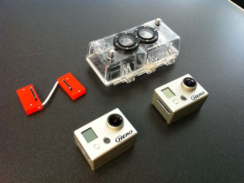
In many areas of oceanographic study measures of the A GO-PRO camera is a fixed focus, 11 mega-pixel, still-
seafloor on a very small scale (capable of resolving variations frame (or 1080p high-definition video) camera measuring just
of just a few mm) are desired. For example, modeling of meso- 42 mm x 60 mm x 30 mm (Fig. 1). Although the camera has no
scale turbulence across the seafloor requires a statistical viewfinder or LCD screen, its small form factor combined with
roughness to accurately predict the bottom boundary layer [1]. a standard waterproof enclosure has made it popular with
Similarly, measurements of seafloor sediment transfer also sports enthusiasts for underwater and extreme sports footage.
depend of the size of the bottom boundary layer and hence, (The camera is frequently mounted to the chest or head while
seafloor roughness [2]. Acoustic remote sensing methods used skiing, surfing, sky diving etc.) A stereo camera kit is available
to characterize the seafloor for habitat and sediment for the GO-PRO camera, which provides a waterproof
composition depend in part of the roughness of the seafloor at enclosure (to 200 ft) for a pair of cameras connected by a
the carrier wavelength of the ensonifying signal [3]. This last synchronization cable for synchronized video or still
application, namely, the characterization of the seafloor by photography. When connected, pairs of cameras take
remote acoustic methods, has led to consideration of methods synchronized still photos and an automatic timer setting allows
for measuring the microbathymetry of the seafloor. the taking of still images at regular intervals (the interval is user
Multibeam echosounders, used throughout the world for the selectable from 2 to 60 sec) without user interaction. The
routine collection of bathymetric data, commonly also collect cameras and kit provided a low cost and easily used system for
co-registered seafloor acoustic backscatter. Acoustic capturing stereo image pairs for micro-bathymetry.
backscatter of the seafloor may be used to characterize the III. CREATING 3D POINT CLOUDS FROM STEREO CAMERA
sediment type [4], the presence of gas, and the likely habitat of PAIRS
many benthic organisms and bottom dwelling fish [5].
However the process of interpreting seafloor backscatter is Stereo cameras take synchronized images of a scene from
complicated by the fact that a large portion of the returned differing vantage points. In general, by knowing the translation
signal at non-normal angles is dependent on the seafloor and rotation of one camera relative to the second, one can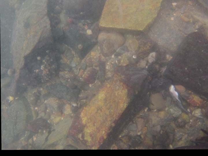
horizontal row fall along an epipolar line. Searches for
                                                                      conjugate pixels between images may then be simplified to a
                                                                      search primarily in one dimension. The distance of a matching
                                                                      pixel in one image relative to the other along each row of
                                                                      rectified images is termed the horizontal disparity which is
                                                                      directly related to the range from the stereo rig to an imaged
                                                                      scene.
                                                                          Rectified images are next resized to 720 x 540 through an
                                                                      averaging process. This step is optional but was undertaken in
                                                                      the preliminary tests to reduce the processing time. The step
                                                                      involves averaging neighboring pixels rather than simple
                                                                      decimation. The distinction is important as decimation aliases
                                                                      high frequency texture components reducing the effectiveness
                                                                      of attempts to match pixels between images. (Processing of full
                                                                      images is possible and will likely result in even a denser point
      Fig. 1. GOPRO Cameras with stereo housing and synchronization   cloud.)
                                   cable.                                 The SIFT algorithm [9] is next used to determine the range
                                                                      of likely disparities between the images and to provide seeds
                                                                      for the subsequent dense matching algorithm. The SIFT
establish the location of an object in 3D space when the object       algorithm creates a Laplacian pyramid of images and utilizes
is uniquely identified in both images. Conjugate pixels in each       the difference of Laplacians to extract points of interest at
image provide pointing vectors from each camera’s focal point         different spatial scales with subpixel accuracy. Extracted points
whose intersection locates the object in question. Challenges to      are then matched across the images using the similarity of
stereo camera reconstruction involve methods to match pixels          descriptors associated with each point to produce a sparse set of
corresponding to common objects in both images.                       matching points. To meet the high-resolution requirements of
    Methods of producing 3D point clouds from stereo camera           this project dense matching is required. Therefore, matches are,
pairs in air are well established [6]. However methods for            when possible, found for all pixels in the image in subsequent
underwater photography are relatively nascent, in part, due to        steps.
the complicating factors related to the light-propagating                 The methodology described above has been developed in
medium. Underwater images often appear blurry due to the              the framework of the project with NOAA South-West Fisheries
scattering effects of water molecules and particles in the water      Science Center with the aim of detection and measurement of
column. Moreover, ambient lighting can be irregular and the           live fishes [10]. In the current work this research has been
displacement between the cameras enhances the effect often            extended by segmenting the rectified images based on their
resulting in different exposures between images. For these            texture [11,12]. The rationale of image segmentation for stereo
reasons, color is, in general, an unreliable metric for matching      processing is that surfaces, which are smoothly varying in 3D
pixels between image pairs. Instead images are converted to           space (and hence in disparity space), are likely to have
gray scale and the resulting image texture proves more reliable.      homogeneous texture and thus appear in the same segment.
    The process of creating 3D point clouds from stereo camera        Also, a sudden change in disparity (due to an occlusion, for
pairs first involves calibration of the camera pair to measure the    example) usually manifests itself as textural or colorimetric
distortion of optical system of each camera (intrinsic                change and thus cause a boundary between neighboring
parameters) and to establish the translational rotational offsets     segments. Segmentation is performed at different levels of
and between their optical axes (extrinsic parameters). The            granularity, and a level with 600-800 segments is selected for
calibration has been done with the Camera Calibration                 further processing. In this case, each segment has area of
Toolbox for MATLAB [7]. Images of a checkerboard pattern              approximately 500 pixels – a sufficient amount to collect
were taken at several orientations. Calibration images are taken      representative histograms and small enough to guarantee an
underwater for accurate compensation for lens distortion on           absence of disparity jumps within a single segment.
subsequent underwater imagery.                                            Each segment is considered separately. For each pixel P0 in
    A pair of images selected for processing are first cropped        a segment a number of potential candidates for its conjugate P0’
and resampled to a smaller size for convenience. GO-PRO               in the other image are chosen. A window of pixels in the
cameras have a field of view of 170 degrees in air. Such a wide       vicinity of P0 and P0’ and within the same segment are selected.
field of view imparts severe distortion to portions of the image      The maximum number of pixels in a window is 7 x 7, but they
near the edges, which are difficult to capture in the calibration     are arranged in variable patterns. The smallest scale consists of
process. One eighth of the image is removed from each side,           a 7 x 7 window, the next scale a 13*13 window, and the last,
reducing a 3840 x 2880 pixel image to 2880 x 2160 pixels.             the 5-th scale a 31 x 31 window. Thus, with the same
    Lens related distortion is then compensated for, and images       calculation complexity the similarity between regions can be
are rectified using standard methods [8]. Rectification produces      detected on a variety of scales. Normalize cross correlation
two images with epipoles at infinity, such that pixels in each        (NCC) scores are calculated for each window. Locations of P0’
with the highest NCC scores are recorded. Pixels with                        roughness is defined as the sum of absolute differences
conjugates detected by SIFT matching are considered to have                  between neighbor disparities divided by number of neighboring
the highest NCC score of 1, but other potential candidates are               pairs of pixels. Practice shows that the correct solution does not
found for them too.                                                          necessarily have the highest NCC score and the lowest
    Next, histograms of disparities for each individual segment              roughness, so discarding all but the best solution might lead to
are constructed. Two histograms are created: one consists of                 a wrong result. Hence if a few top solutions minimizing the
only top-scoring candidates, while the second contains all                   transition from seed values have comparable scores they are all
recorded candidates for all pixels in the segment. In most cases             kept to make the final decision at a final stage.
disparities for incorrect matches are distributed uniformly                       When histograms of disparities within a segment,
within the search range, while correct disparities are localized             comparison with SIFT determined seeds, amplitude of NCC
in a narrow interval, so that each histogram has a distinct peak.            scores and local roughness of NCC scores all fail to definitively
When the texture in the image is rich and distinct, the                      resolve the correct disparity, the candidates are compared to
histogram of top scorers usually contains a single peak                      those in adjacent segments. Disparity ranges in successful
corresponding to the correct match for the segment as a whole.               segments neighboring the one with several equally good
However when the texture is not well pronounced the                          solutions are compared. Again the assumption of local
histogram of top scorers is less reliable. In this case a histogram          smoothness is utilized. The investigated segment is likely to
of all recorded candidates better represent the disparity of the             have smooth transition of disparities with the majority of its
segment. Both histograms are processed and the dominant                      neighbors. If this condition is not fulfilled for any of the kept
peaks are determined. In the case of a single, co-located peak in            solutions the segment is considered an outlier and invalidated
both histograms, it is accepted as a final solution for a segment.           (its pixels are not used in triangulation).
In cases of several peaks with comparable dominance each                          Methods described thus far determine the disparity between
associated solution is investigated individually.                            matching pixels in the two images with the resolution of a
    To resolve cases of multiple histogram peaks showing no                  single pixel. To gain subpixel resolution, a parabola is fit to the
agreement to the correct disparity the candidate values are                  disparities of neighboring pixels centered on the pixel of
compared to the seed values (from SIFT matching). First                      interest and the peak of the paraboloid is chosen for the final
disparities corresponding to the seed values and those                       disparity measure.
corresponding to the peak maximum are set. In an iterative                        The camera calibration along with the calculated disparities
process, the neighboring disparities for resolved disparities are            between matching pixels are used to calculate the location of
chosen such that the difference with already set values are                  each object in 3D space by triangulating the intersection which
minimized, resulting in the smoothest possible solution. As a                originate at each camera’s focal point and whose direction is
check of these results two quantitative characteristics are                  determined by their disparity using standard methods [6].
considered: average NCC score of chosen disparities and                      These results produce a point cloud, which is used to generate
average roughness of disparities within a segment, where                     the surfaces presented in the next section.
                                                                                                       IV. RESULTS
                          Image of Towel and Carpet.                             Preliminary tests were conducted in air to test the setup and
                                                                             method. Figure 1 shows the left camera image of an office
                                                                             carpet and blue towel laid flat on the surface. Figure 2a shows a
                                                                             3 mm x 3 mm median grid of the point cloud data after
                                                                             subtracting the point heights from a plane fit to the portion of
                                                                             the data associated with the carpet. The RMS deviation of the
                                                                             data to the plane is 9 mm. Careful examination of the surface
                                                                             shows two artifacts. The first is a slight curvature to the surface
                                                                             revealed as a lightening of the gray-scale shaded image in the
                                                                             center of the grid. This curvature results from an imperfect
                                                                             correction for lens distortion and was left uncorrected for to
                                                                             illustrate the effect. The second is a small 5 mm irregularity in
                                                                             the surface creating bands in the gray-scale height. This results
                                                                             from an inability of the sub-pixel disparity algorithm to
    Fig. 2. One of a pair of stereo camera images used for initial in-air    discriminate disparities at the sub-pixel level for the textures
         testing of the system’s ability to generate dense 3D point clouds   provided by these surfaces.
                               of textured surfaces.
Image of Pen on Wet Beach
Fig. 5. One of a pair of stereo camera images used for initial in-air
testing of the system’s ability to generate dense 3D point
a) clouds. Here a pen was laid on a sandy beach to further test the
resolving capability of the method.
b) a)
Fig. 4. The surface in a) is a grid of the residuals to a plane fit to the
3D point cloud calculated from stereo reconstruction of the
towel and carpet scene shown in Figure 2. A cross-section of
the surface is shown in b) showing the towel’s 7 mm height
relative to the floor. Residual curvature in the surface results
from an imperfect camera calibration, left uncorrected to
illustrate the effect.
Figure 2b shows a cross-section of the data set in which the
towel is clearly visible as a 7 mm increase in surface height at a
distance of 150 mm from the edge of the plot. While errors in
our calibration methods left residual curvature to the surface
these results were sufficiently promising to continue
investigation of the method.
Figure 4 shows the left image for a second test photo in air,
in which a pen was imaged on a wet sandy beach. The grain b)
size and texture of the beach provided a means to test the
algorithms in a real-world scenario and to adjust the methods to Fig. 3. The surface in a) is a 3 mm grid of the 3D point cloud
calculated from stereo reconstruction of the beach and pen
obtain the best image for stereo reconstruction. Here the pen is
scene in Fig. 4. A cross-section of the surface is shown in b)
clearly recognizable in the surface plot and cross-section where the pen is clearly evident as a 1 cm bump on the
provided in Figures 5a and 5b respectively. surface.Point Cloud Density
Underwater Test Image
50
40
Count, 1000s
30
20
10
0
0 10 20 30 40 50
Number of Points Per 3 mm Grid Cell
a) a)
b)
b)
Fig. 6. After underwater calibration of the stereo system, an
Fig. 7. Here the number of points per 3 mm grid node and their underwater scene was taken shown in a) above. A 3 mm grid
standard deviation are plotted for the surface shown in Fig. of the resulting point cloud is shown in b).
4a. The images used for this reconstruction were taken at
approximately 0.7 m above the surface and were decimated
by a factor of 4 prior to stereo reconstruction.
(and therefore have not texture) or are occluded from the view
of either camera produce outliers. These are shown as small
white patches in this vertical view of the surface as the outliers
Figures 6a and 6b show the number of data points per grid are invariably shallow with respect to the surface and off the
node and their standard deviation respectively for this image. color scale. Objects on the order of 1 cm are resolved, although
The image was taken approximately 0.7 m from the surface, spaces between objects are often smoothed, in part due to the
which is commensurate with the altitude from which we expect gridding algorithm.
to take images in subsequent field experiments, allowing for
adequate light and water clarity. While the surfaces generated
from stereo image pairs can be noisy, dense matching of all
available pixels generally provides sufficient data density to V. CONCLUSION
remove much of the noise in subsequent averaging. A GO-PRO underwater camera stereo camera rig has been
Figures 7a and 7b show an underwater test image and the used to generate 3 mm resolution grids of seafloor bathymetry
resulting surface generated from the stereo reconstruction. The for the purposes of seafloor characterization. Measurements at
cameras were recalibrated underwater for this test and although this scale allow characterization of the micro-roughness of an
no man-made structures exist in this image to provide a area, which is critical in the modeling of many processes
measure that the scene is generated correctly, a qualitative including laminar and turbulent flow, seafloor sediment
analysis is possible. Major features (large stones and cobles) in transport and acoustic backscatter.
the scene are well represented. Segments that fall in a shadowImages taken less than 1 m from the surface with an [9] D. G. Lowe, “Distinctive Image Features from Scale-Invariant
orientation nearly normal were found to provide adequate Keypoints,” International Journal of Computer Vision, vol. 60,
resolution and uniform density of the resulting point cloud. no. 2, pp. 91–110, 2004.
Underwater stereo imagery is generally more challenging than [10] Y. Rzhanov and G. Cutter, “StereoMeasure and StereoFeatures:
that in air, as light emanating from a point on the seafloor is measuring fish and reconstructing scenes using underwater
scattered by the water column producing blurring or hazing stereo photographs,” National Marine Fisheries Service, Seattle,
Washington, NOAA Technical Memorandum NMFS-F/SPO-
effect that complicates matching of pixels between images.
121, Sep. 2010.
This blurring effect combined with homogeneous fine grain
[11] Y. Deng and B. S. Manjunath, “Unsupervised segmentation of
sediments (silt and mud) requires images as close as 20-30 cm
color-texture regions in images and video,” IEEE Transactions
for the cameras to resolve individual grains for matching. Large on Pattern Analysis and Machine Intelligence, vol. 23, no. 8, pp.
objects imaged from a stereo camera pair produce typically 800 –810, Aug. 2001.
produce rich texture, but complicate processing with occlusions [12] L. Prasad and A. N. Skourikhine, “Vectorized image
(portions of a scene viewable in one image but not in the other) segmentation via trixel agglomeration,” Pattern Recognition,
which produce outliers. vol. 39, no. 4, pp. 501–514, Apr. 2006.
The GO-PRO underwater camera stereo system is not
found to be ideal, having a quite short baseline (3.5 cm), which
limits resolution of the resulting point cloud. When the scene
has poor texture the sub-pixel algorithm used here can fail to
improve the resolution of the system beyond that produced by
the baseline alone. The final point cloud may appear to have
discrete steps corresponding to integer pixel disparities as a
result. Moreover, the cameras require high light levels to take
adequately illuminated images. At deeper depths artificial
lighting may be required. None-the-less, great convenience is
found in the relatively low cost, prepackaged system and
measures of seafloor micro-bathymetry capable of resolving
seafloor features less than 1 cm in amplitude were possible.
VI. ACKNOWLEDGEMENT
This work was funded by NOAA Grants
NA05NOS4001153 and NA10NOS4000073
VII. REFERENCES
[1] R. G. Dean and R. A. Dalrymple, Water wave mechanics for
engineers and scientists. World Scientific, 1991.
[2] R. G. Dean and R. A. Dalrymple, Coastal Processes with
Engineering Applications. Cambridge University Press, 2004.
[3] X. Lurton, An Introduction to Underwater Acoustics: Principles
and Applications, 2nd ed. Springer, 2010.
[4] Fonseca and L. Mayer, “Remote estimation of surficial seafloor
properties through the application Angular Range Analysis to
multibeam sonar data,” Mar Geophys Res, vol. 28, no. 2, pp.
119–126, Jun. 2007.
[5] P. T. Harris and E. K. Baker, Seafloor Geomorphology as
Benthic Habitat: GeoHAB Atlas of Seafloor Geomorphic
Features and Benthic Habitats. Elsevier, 2011.
[6] R. Hartley and A. Zisserman, Multiple view geometry in
computer vision. Cambridge, UK; New York: Cambridge
University Press, 2003.
[7] J.-Y. Bouguet, Camera Calibration Toolbox for MATLAB,
http://www.vision.caltech.edu/bouguetj/calib_doc/.
[8] A. Fusiello, E. Trucco, and A. Verri, “A compact algorithm for
rectification of stereo pairs,” Machine Vision and Applications,
vol. 12, no. 1, pp. 16–22, 2000.You can also read