Methane emissions in the United States, Canada, and Mexico: evaluation of national methane emission inventories and 2010-2017 sectoral trends by ...
←
→
Page content transcription
If your browser does not render page correctly, please read the page content below
Research article
Atmos. Chem. Phys., 22, 395–418, 2022
https://doi.org/10.5194/acp-22-395-2022
© Author(s) 2022. This work is distributed under
the Creative Commons Attribution 4.0 License.

        Methane emissions in the United States, Canada, and
          Mexico: evaluation of national methane emission
        inventories and 2010–2017 sectoral trends by inverse
       analysis of in situ (GLOBALVIEWplus CH4 ObsPack) and
             satellite (GOSAT) atmospheric observations
            Xiao Lu1,2,16 , Daniel J. Jacob2 , Haolin Wang1 , Joannes D. Maasakkers3 , Yuzhong Zhang2,4,5 ,
         Tia R. Scarpelli2 , Lu Shen2 , Zhen Qu2 , Melissa P. Sulprizio2 , Hannah Nesser2 , A. Anthony Bloom6 ,
       Shuang Ma6 , John R. Worden6 , Shaojia Fan1 , Robert J. Parker7,8 , Hartmut Boesch7,8 , Ritesh Gautam9 ,
        Deborah Gordon10,11 , Michael D. Moran12 , Frances Reuland13 , Claudia A. Octaviano Villasana14 , and
                                                     Arlyn Andrews15
              1 School   of Atmospheric Sciences, Sun Yat-sen University, Zhuhai, Guangdong Province, China
               2 Harvard     John A. Paulson School of Engineering and Applied Sciences, Harvard University,
                                                        Cambridge, MA, USA
                            3 SRON Netherlands Institute for Space Research, Utrecht, the Netherlands
                      4 School of Engineering, Westlake University, Hangzhou, Zhejiang Province, China
                   5 Institute of Advanced Technology, Westlake Institute for Advanced Study, Hangzhou,

                                                      Zhejiang Province, China
                      6 Jet Propulsion Laboratory, California Institute of Technology, Pasadena, CA, USA
                         7 National Centre for Earth Observation, University of Leicester, Leicester, UK
         8 Earth Observation Science, Department of Physics and Astronomy, University of Leicester, Leicester, UK
                                       9 Environmental Defense Fund, Washington, DC, USA
                                                    10 RMI, New York, NY, USA
               11 Watson Institute for International and Public Affairs, Brown University, Providence, RI, USA
                                12 Environment and Climate Change Canada, Toronto, ON, Canada
                                                     13 RMI, Boulder, CO, USA
                    14 Instituto Nacional de Ecología y Cambio Climático (INECC), Mexico City, Mexico
       15 National Oceanic and Atmospheric Administration, Earth System Research Laboratory, Boulder, CO, USA
      16 Guangdong Provincial Observation and Research Station for Climate Environment and Air Quality Change in

                                    the Pearl River Estuary, Zhuhai, Guangdong Province, China
                                Correspondence: Xiao Lu (luxiao25@mail.sysu.edu.cn)

                                 Received: 10 August 2021 – Discussion started: 19 August 2021
                    Revised: 12 November 2021 – Accepted: 29 November 2021 – Published: 12 January 2022

      Abstract. We quantify methane emissions and their 2010–2017 trends by sector in the contiguous United States
      (CONUS), Canada, and Mexico by inverse analysis of in situ (GLOBALVIEWplus CH4 ObsPack) and satellite
      (GOSAT) atmospheric methane observations. The inversion uses as a prior estimate the national anthropogenic
      emission inventories for the three countries reported by the US Environmental Protection Agency (EPA), En-
      vironment and Climate Change Canada (ECCC), and the Instituto Nacional de Ecología y Cambio Climático
      (INECC) in Mexico to the United Nations Framework Convention on Climate Change (UNFCCC) and thus
      serves as an evaluation of these inventories in terms of their magnitudes and trends. Emissions are optimized
      with a Gaussian mixture model (GMM) at 0.5◦ × 0.625◦ resolution and for individual years. Optimization is

Published by Copernicus Publications on behalf of the European Geosciences Union.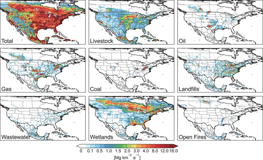
396                                              X. Lu et al.: Methane emissions in the United States, Canada, and Mexico

       done analytically using lognormal error forms. This yields closed-form statistics of error covariances and infor-
       mation content on the posterior (optimized) estimates, allows better representation of the high tail of the emission
       distribution, and enables construction of a large ensemble of inverse solutions using different observations and
       assumptions. We find that GOSAT and in situ observations are largely consistent and complementary in the op-
       timization of methane emissions for North America. Mean 2010–2017 anthropogenic emissions from our base
       GOSAT + in situ inversion, with ranges from the inversion ensemble, are 36.9 (32.5–37.8) Tg a−1 for CONUS,
       5.3 (3.6–5.7) Tg a−1 for Canada, and 6.0 (4.7–6.1) Tg a−1 for Mexico. These are higher than the most recent
       reported national inventories of 26.0 Tg a−1 for the US (EPA), 4.0 Tg a−1 for Canada (ECCC), and 5.0 Tg a−1 for
       Mexico (INECC). The correction in all three countries is largely driven by a factor of 2 underestimate in emis-
       sions from the oil sector with major contributions from the south-central US, western Canada, and southeastern
       Mexico. Total CONUS anthropogenic emissions in our inversion peak in 2014, in contrast to the EPA report of a
       steady decreasing trend over 2010–2017. This reflects offsetting effects of increasing emissions from the oil and
       landfill sectors, decreasing emissions from the gas sector, and flat emissions from the livestock and coal sectors.
       We find decreasing trends in Canadian and Mexican anthropogenic methane emissions over the 2010–2017 pe-
       riod, mainly driven by oil and gas emissions. Our best estimates of mean 2010–2017 wetland emissions are 8.4
       (6.4–10.6) Tg a−1 for CONUS, 9.9 (7.8–12.0) Tg a−1 for Canada, and 0.6 (0.4–0.6) Tg a−1 for Mexico. Wetland
       emissions in CONUS show an increasing trend of +2.6 (+1.7 to +3.8)% a−1 over 2010–2017 correlated with
       precipitation.

1   Introduction                                                   methane measurements from ground, aircraft, and satellite
                                                                   platforms show larger methane emissions than reported in the
Atmospheric methane (CH4 ) is the most important anthro-           GHGI, particularly for the oil and gas industry (Alvarez et al.,
pogenic greenhouse gas after carbon dioxide (CO2 ). Nat-           2018; Zhang et al., 2020; Lu et al., 2021; Maasakkers et al.,
ural emissions are mainly from wetlands. Anthropogenic             2021; Qu et al., 2021) and for livestock (Lu et al., 2021; Yu
emissions are from many sectors including the oil and gas          et al., 2021). Atmospheric observations also suggest an in-
supply chain, coal mining, livestock, and waste manage-            creasing trend of US anthropogenic emissions over the past
ment. Individual countries must report their anthropogenic         decade (Turner et al., 2016; Sheng et al., 2018a; Lan et al.,
methane emissions by sector to the United Nations in ac-           2019; Maasakkers et al., 2021), while the GHGI indicates a
cordance with the United Nations Framework Convention on           decrease (EPA, 2021).
Climate Change (UNFCCC, 1992). These national emission                Anthropogenic methane emissions for Canada are re-
inventories are mainly constructed by bottom-up methods as         ported yearly by Environment and Climate Change Canada
the product of activity data and emission factors, following       (ECCC, 2020a; 2021) as part of the National Inventory Re-
methodological guidelines from the Intergovernmental Panel         port (NIR). Atmospheric observations again indicate an un-
on Climate Change (IPCC). The emission factors are highly          derestimate of emissions from oil and gas production (Ather-
variable and have large uncertainties, leading to errors in        ton et al., 2017; Johnson et al., 2017; Chan et al., 2020; Baray
estimating national emissions, their trends, and the contri-       et al., 2021; Lu et al., 2021; Tyner and Johnson, 2021) but a
butions of different sectors (Kirschke et al., 2013; Saunois       decrease in these emissions over the past decade (Lu et al.,
et al., 2020). Top-down methods involving inversion of at-         2021; Maasakkers et al., 2021). Scarpelli et al. (2021) re-
mospheric methane observations can usefully diagnose these         cently allocated the ECCC NIR (ECCC 2020a) for the year
errors (Houweling et al., 2017). Here, we use an inverse anal-     2018 on a 0.1◦ × 0.1◦ grid, and our work is the first to use it
ysis of 2010–2017 in situ and satellite observations of at-        in an inverse analysis.
mospheric methane over North America to evaluate national             Mexico’s anthropogenic methane emissions are reported
emission inventories and their trends by sector for the United     by the Instituto Nacional de Ecología y Cambio Climático
States (US), Canada, and Mexico.                                   (INECC) in Mexico’s National Inventory of Greenhouse
   US anthropogenic methane emissions are reported yearly          Gases and Compounds (INEGyCEI) for selected years (IN-
by the US Environmental Protection Agency (EPA, 2021)              ECC and SEMARNAT, 2018). The last communication to
as part of the Inventory of US Greenhouse Gas Emissions            the UNFCCC was in 2015, and this inventory was allocated
and Sinks (GHGI). Methane emissions for the year 2012,             to a 0.1◦ × 0.1◦ grid by Scarpelli et al. (2020). A recent in-
from the 2016 version of this inventory (EPA, 2016), were          verse analysis of satellite data finds oil and gas emissions to
spatially allocated on a 0.1◦ × 0.1◦ (10 × 10 km) grid by          be underestimated by a factor of 2 over eastern Mexico (Shen
Maasakkers et al. (2016) to enable its evaluation using            et al., 2021).
top-down methods. Results using analysis of atmospheric

Atmos. Chem. Phys., 22, 395–418, 2022                                                 https://doi.org/10.5194/acp-22-395-2022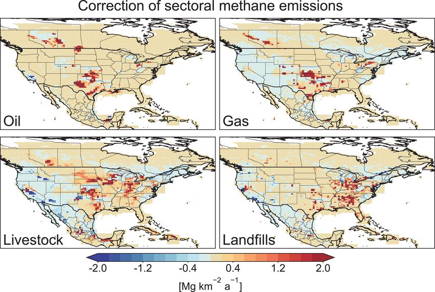
X. Lu et al.: Methane emissions in the United States, Canada, and Mexico 397
The above top-down studies, except for Baray et al. (2021) tegration Project, 2019). Following Lu et al. (2021), data
and Lu et al. (2021), used either in situ or satellite obser- from surface and tower sites are sampled only during daytime
vations but not both. Satellite observations have better data (10:00–16:00 LT) and averaged as daytime mean values on
coverage but are less sensitive to emissions (Turner et al., individual days for use in the inversion. For sites with stan-
2018) and have larger uncertainties, particularly at high lat- dard deviations larger than 30 ppb, we exclude data points
itudes. In a previous inverse analysis (Lu et al., 2021), we that depart by more than 2 standard deviations from the mean
showed that in situ and satellite observations provide comple- because such local extreme conditions are difficult to simu-
mentary global information for inverse analyses of methane late with the chemical transport model. For other sites we
emissions. That inversion was conducted at 4◦ × 5◦ resolu- exclude data points that depart by more than 3 standard de-
tion, which is too coarse for specific evaluation of national viations from the mean. We also exclude aircraft measure-
inventories. ments higher than 9 km a.s.l. as these measurements would
Here we apply extensive in situ observations from sur- have weak sensitivity to surface fluxes.
face sites, towers, ships, and aircraft (GLOBALVIEWplus The in situ observations thus include 49 742 data points
CH4 ObsPack data compilation) together with the Green- from surface sites, 15 285 from towers, 56 from ship cruises,
house Gases Observing Satellite (GOSAT) observations in and 26 620 from aircraft campaigns over North America and
an inverse analysis for 2010–2017 to optimize methane emis- adjacent waters (Fig. 1a). The number of available in situ ob-
sions and their year-to-year variability at up to 0.5◦ × 0.625◦ servations per year increases from 10 830 in 2010 to 13 593
resolution for North America. We use as prior estimates the in 2017. All these in situ data points are used in the base in-
gridded national emission inventories from the EPA (US), version to optimize methane emissions for individual years.
ECCC (Canada), and INECC (Mexico) so that our results We also conduct sensitivity inversions by only using surface
can inform inventory improvement planning at the emission and tower sites with continuous 8-year records for trend anal-
sector level. Following Lu et al. (2021), we use an analytical yses.
inversion method that provides closed-form characterization
of error statistics and information content on the inverse so- 2.2 GOSAT satellite methane observations
lution and that also allows us to quantitatively compare the
information from the in situ and satellite observations. The GOSAT satellite launched in 2009 measures the
backscattered solar radiation from a sun-synchronous or-
2 Methods bit at around 13:00 LT (Kuze et al., 2016). Methane is re-
trieved in the 1.65 µm shortwave infrared absorption band.
We use methane observations from the GLOBALVIEWplus We use the column-averaged dry-air methane mixing ratios
CH4 ObsPack in situ data (Sect. 2.1) and/or GOSAT satellite from the University of Leicester version 9.0 Proxy XCH4 re-
retrievals (Sect. 2.2) with the GEOS-Chem chemical trans- trieval (Parker et al., 2020a). Comparison with ground-based
port model (Sect. 2.4) as the forward model to optimize a methane observations from the Total Carbon Column Ob-
state vector of mean methane emissions for individual years serving Network (TCCON) shows that the retrieval has a
(Sect. 2.3) covering the North American continent at a spatial single-observation precision of 13 ppb and an overall global
resolution of up to 0.5◦ × 0.625◦ . We derive posterior esti- bias of 9 ppb that is removed from the Proxy XCH4 data
mates of the state vector and the associated error covariance (Parker et al., 2020a). Here we use a total of 205 875 (25 734
matrix by analytical solution to the Bayesian optimization per year on average) GOSAT retrievals for 2010–2017 over
problem (Sect. 2.5). Our base inversion uses GOSAT + in North America in the inversion, excluding glint data over the
situ observations and our best choices of inversion param- oceans and data poleward of 60◦ , which are not representa-
eters. We also present results from an ensemble of sensitivity tively sampled and for which errors are large (Fig. 1b).
inversions using observation subsets (in situ or GOSAT) and
varying inversion parameter assumptions (e.g., different er- 2.3 Prior emission inventories
ror distributions). We attribute inversion results to different
methane emission sectors with the methodology described in We use as prior estimates of anthropogenic methane emis-
Sect. 2.6. sions the gridded versions of the official national invento-
ries for the US (EPA, 2016), Canada (ECCC, 2020a), and
Mexico (INECC and SEMARNAT, 2018) (Maasakkers et al.,
2.1 In situ methane observations
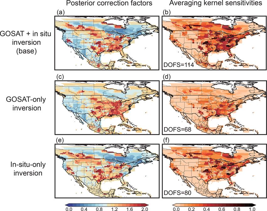
2016; Scarpelli et al., 2020, 2021). These emissions are listed
We use the comprehensive database of in situ (surface, tower, in Table 1 for individual countries, and the spatial distribu-
shipboard, and aircraft) methane observations over North tions for major sectors are shown in Fig. 2. We assume no
America for 2010–2017 from the GLOBALVIEWplus CH4 year-to-year trend in the prior emissions so that trends from
ObsPack v1.0 product compiled by the National Oceanic the inversion are solely driven by observations. Prior an-
and Atmospheric Administration (NOAA) Global Monitor- thropogenic emissions for the contiguous US (CONUS) are
ing Laboratory (Cooperative Global Atmospheric Data In- 28.7 Tg a−1 . Anthropogenic US emissions outside CONUS
https://doi.org/10.5194/acp-22-395-2022 Atmos. Chem. Phys., 22, 395–418, 2022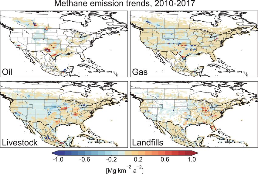
398                                                 X. Lu et al.: Methane emissions in the United States, Canada, and Mexico

Figure 1. Methane observations over North America used in the inversion. The observations are from the in situ GLOBALVIEWplus CH4
ObsPack data product and from the GOSAT satellite instrument. Mixing ratios shown for surface, tower, and GOSAT observations are means
for 2010–2017. Aircraft and shipboard observation locations are shown as additional symbols. The GOSAT data are dry column mixing
ratios from the University of Leicester version 9 Proxy XCH4 retrieval (Parker et al., 2020a) and are averaged here on the 0.5◦ × 0.625◦
GEOS-Chem model grid.

(mostly Alaska, not optimized in the inversion) account for           2.4   The GEOS-Chem forward model
only 0.3 Tg a−1 according to Maasakkers et al. (2016). The
latest GHGI report from the EPA (2021) gives mean emis-
                                                                      We use the nested version of the GEOS-Chem 12.5.0
sions of 26.0 Tg a−1 for 2010–2017. Prior anthropogenic
                                                                      chemical transport model (http://geos-chem.org, last access:
emissions for Canada are 3.7 Tg a−1 . The most recent 2021
                                                                      6 April 2021) (Wecht et al., 2014) as the forward model for
version of the ECCC NIR gives a mean of 4.0 Tg a−1 for
                                                                      the inversion. The model is driven by MERRA-2 re-analysis
2010–2017 (ECCC, 2021). Mexico anthropogenic emissions
                                                                      meteorological fields at their native 0.5◦ × 0.625◦ resolution
are 5.0 Tg a−1 , and 2015 is the latest available year from IN-
                                                                      (Gelaro et al., 2017). Methane loss from atmospheric oxida-
ECC.
                                                                      tion is as described in Lu et al. (2021) but is inconsequential
   Prior methane emissions from wetlands are the 0.5◦ ×0.5◦
                                                                      here because it is negligibly slow compared to the timescale
gridded mean monthly values for 2010–2017 from the nine
                                                                      for ventilation of the North American domain. Soil uptake
highest-performance members of the WetCHARTs v1.3.1 in-
                                                                      of methane is from the MeMo model v1.0 (Murguia-Flores
ventory ensemble (Ma et al., 2021), selected for their fit to
                                                                      et al., 2018) but is very small and therefore not optimized in
the global GOSAT inversion results of Zhang et al. (2021).
                                                                      the inversion.
This choice of prior estimate effectively corrects the large
                                                                         The GEOS-Chem model simulation is conducted at 0.5◦ ×
overestimates of wetland emissions for North America previ-
                                                                      0.625◦ resolution over the North America domain (130–
ously found in inversions of GOSAT and aircraft data when
                                                                      55◦ W, 15–65◦ N) (Fig. 1) for the 2010–2017 period, with dy-
using the overall mean of the WetCHARTs v1.0 ensemble
                                                                      namic boundary conditions archived every 3 h from a global
(Sheng et al., 2018b; Maasakkers et al., 2021). We do not
                                                                      2010–2017 simulation at 4◦ × 5◦ resolution using methane
include interannual variability from WetCHARTs because it
                                                                      emissions and sinks previously optimized with GOSAT ob-
is highly uncertain and we prefer to have it informed by the
                                                                      servations (Lu et al., 2021). This means that GOSAT ob-
observations. Unlike in our global inversion (Lu et al., 2021),
                                                                      servations over North America are used twice: once for the
we do not optimize the relative seasonal variation of wetland
                                                                      global inversion (along with other observations worldwide)
emissions and instead have it imposed by the prior estimate
                                                                      and once for the North American inversion, but this is in-
(Parker et al., 2020b). Prior estimates of open fire emissions
                                                                      consequential because the sole purpose of the global opti-
are the daily values for individual years from the Global Fire
                                                                      mization is to avoid biases in boundary conditions that would
Emissions Database (GFED) version 4s (van der Werf et al.,
                                                                      cause spurious corrections to emissions within the inversion
2017). Other small natural emissions (seepages, termites) are
                                                                      domain (Wecht et al., 2014). Lu et al. (2021) show that their
as described in Lu et al. (2021).
                                                                      optimized simulation is unbiased in comparison to global
                                                                      zonal mean observations for 2010–2017, but we still find
                                                                      some residual biases for individual years up to 5 ppbv. We
                                                                      therefore optimize the mean boundary conditions for indi-
                                                                      vidual years on each side of the domain (north, south, west,
                                                                      east) as part of the North American inversion. The initial
                                                                      methane concentration fields on 1 January 2010 are from Lu
                                                                      et al. (2021), which have been adjusted to have an unbiased

Atmos. Chem. Phys., 22, 395–418, 2022                                                     https://doi.org/10.5194/acp-22-395-2022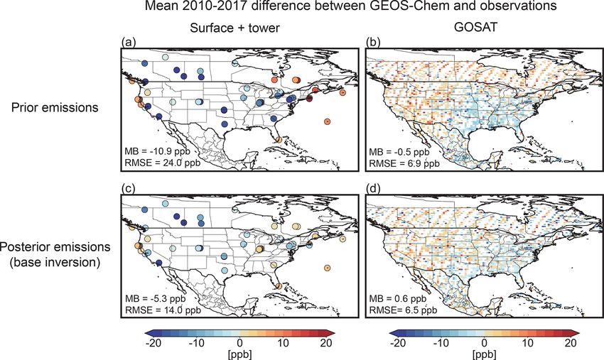
X. Lu et al.: Methane emissions in the United States, Canada, and Mexico                                                                       399

Table 1. (a) Mean 2010–2017 methane emissions for the contiguous US (CONUS).

                                                                         Priora               Posteriorb        Sensitivityc
                                Total sources [Tg a−1 ]                    36.8      46.3 (40.2–48.4)                     0.72
                                     Anthropogenic sources               28.7d       36.9 (32.5–37.8)                     0.55
                                     Livestock                              9.2       10.6 (9.2–11.8)                     0.43
                                     Oil                                    2.3          4.6 (3.0–4.7)                    0.43
                                     Natural gas                            6.8         9.9 (8.1–10.5)                    0.42
                                     Coal mining                            2.9          2.8 (2.4–3.5)                    0.44
                                     Landfills                              5.8          7.2 (6.0–7.6)                    0.34
                                     Wastewater                            0.70      0.63 (0.56–0.74)                     0.57
                                     Rice cultivation                      0.48      0.65 (0.49–0.68)                     0.33
                                     Other anthropogenic                   0.46      0.45 (0.44–0.54)                     0.30
                                     Natural sources                        8.6         9.5 (7.4–11.5)                    0.64
                                     Wetlands                               7.5        8.4 (6.4–10.6)                    0.57
                                     Open fires                            0.16      0.17 (0.15–0.24)                    0.43
                                     Termites                              0.59      0.63 (0.57–0.76)                   < 0.1
                                     Seeps                                 0.28      0.27 (0.23–0.35)                    0.14
                              a Prior estimates for the inversion. Anthropogenic emissions are from the Environmental
                              Protection Agency (EPA) Inventory of US Greenhouse Gas Emissions and Sinks (GHGI) for the
                              year 2012 as reported by the EPA (2016). Wetland emissions are the 2010–2017 mean of the
                              high-performance subset of the WetCHARTs ensemble (Ma et al., 2021). Open fire emissions
                              are from GFEDv4s (van der Werf et al., 2017). Termite and seep emissions are as described in
                              Lu et al. (2021).
                              b Results from the base inversion of GOSAT and GLOBALVIEWplus data, with the range from
                              the inversion ensemble and from the two sectoral attribution methods (66 total ensemble
                              members) in parentheses.
                              c Sensitivity of the posterior estimate to the observations as diagnosed by the diagonal elements
                              of the averaging kernel matrix, ranging from 0 (no sensitivity, posterior equal to prior) to 1 (full
                              sensitivity, posterior fully determined by the observations). Values are from the base inversion
                              for the year 2015. Results for other years show similar values. See Sect. 2.6 for more details.
                              d The most recent EPA GHGI report (EPA, 2021) gives a mean anthropogenic emission of
                              26.0 Tg a−1 for 2010–2017. Anthropogenic US emissions outside CONUS (mostly Alaska)
                              account for only 0.3 Tg a−1 according to the EPA (Maasakkers et al., 2016) and are not
                              optimized in the inversion.

zonal mean relative to GOSAT observations such that model                          distribution of methane emissions for different sectors as
discrepancies with observations over our 2010–2017 simu-                           given by the prior estimates. Optimal construction of the
lation period can be attributed to model errors in emissions                       GMM aggregates regions with weak or homogeneous emis-
instead of errors in initial conditions.                                           sions while preserving native resolution for strong localized
                                                                                   source regions. The Gaussian functions overlap, providing
                                                                                   additional high-resolution structure in the inverse solution on
2.5   Inversion procedure                                                          the 0.5◦ ×0.625◦ native grid. The state vector x for individual
                                                                                   years is defined as the emission of each of the 600 Gaussians,
Our state vector x to be optimized in the inversion includes
                                                                                   plus the correction to the model boundary conditions as de-
spatially resolved emissions in North America and bound-
                                                                                   scribed earlier, for a total dimension n = 604.
ary conditions for each year of 2010–2017. Although we
                                                                                      The inversion finds the optimal estimate of x by minimiz-
could technically optimize methane emissions for each of
                                                                                   ing the Bayesian cost function J (x) (Brasseur and Jacob,
the 0.5◦ × 0.625◦ native model grid elements, the observa-
                                                                                   2017):
tions do not have sufficient coverage to constrain emissions
everywhere at that resolution, and doing so would intro-                           J (x) =(x − x A )T S−1
                                                                                                       A (x − x A )
duce large smoothing errors in the inversion (Wecht et al.,
                                                                                               + γ (y − F(x))T S−1
                                                                                                                O (y − F(x)),                   (1)
2014). Following Turner and Jacob (2015) and Maasakkers
et al. (2021), we use instead a Gaussian mixture model                             where x A is the prior estimate of x, SA denotes the prior er-
(GMM) to determine the emission patterns that can be con-                          ror covariance matrix, y is the observation vector, SO denotes
strained effectively by the inversion. This is done by project-                    the observation error covariance matrix, γ is a regularization
ing the native-resolution methane emissions onto 600 Gaus-                         factor (see below), and F(x) represents the GEOS-Chem sim-
sian functions optimized to fit the location, magnitude, and                       ulation of y. The GEOS-Chem forward model F(x) as imple-

https://doi.org/10.5194/acp-22-395-2022                                                                       Atmos. Chem. Phys., 22, 395–418, 2022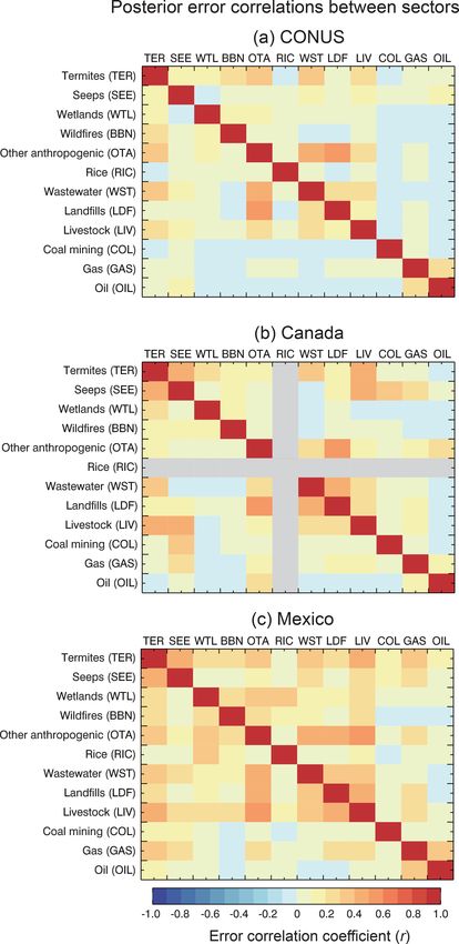
400                                                       X. Lu et al.: Methane emissions in the United States, Canada, and Mexico

Table 1. (b) Mean 2010–2017 methane emissions for Canada.

                                                                         Priora               Posteriorb        Sensitivityc
                                Total sources [Tg a−1 ]                    17.1      16.2 (13.5–17.4)                     0.60
                                     Anthropogenic sources                    3.7         5.3 (3.6–5.7)                   0.59
                                     Livestock                             1.1          1.4 (1.0–1.6)                     0.48
                                     Oil                                  0.75         1.8 (0.81–1.9)                     0.48
                                     Natural gas                          0.80         1.1 (0.76–1.6)                     0.54
                                     Coal mining                         < 0.1                  < 0.1                     0.51
                                     Landfills                            0.66       0.69 (0.45–0.74)                     0.33
                                     Wastewater                          < 0.1                  < 0.1                     0.20
                                     Rice cultivation                        0                      0                        /
                                     Other anthropogenic                  0.27       0.31 (0.26–0.36)                     0.18
                                     Natural sources                       13.5        10.9 (8.7–13.2)                    0.54
                                     Wetlands                             12.0         9.9 (7.8–12.0)                    0.57
                                     Open fires                            1.1       0.67 (0.48–0.95)                    0.54
                                     Termites                             0.28       0.29 (0.24–0.30)                   < 0.1
                                     Seeps                               < 0.1                  < 0.1                   < 0.1
                              a Prior estimates for the inversion. Anthropogenic emissions are from the Environment and
                              Climate Change Canada (ECCC) National Inventory Report (NIR) for the year 2018 (ECCC,
                              2020). Wetland emissions are the 2010–2017 mean of the high-performance subset of the
                              WetCHARTs ensemble (Ma et al., 2021). Open fire emissions are from GFEDv4s (van der Werf
                              et al., 2017). Termite and seep emissions are as described in Lu et al. (2021).
                              b Results from the base inversion of GOSAT and GLOBALVIEWplus in situ data, with the
                              range from the inversion ensemble and from the two sectoral attribution methods (66 total
                              ensemble members) in parentheses.
                              c Sensitivity of the posterior estimate to the observations as diagnosed by the diagonal elements
                              of the averaging kernel matrix, ranging from 0 (no sensitivity, posterior equal to prior) to 1 (full
                              sensitivity, posterior fully determined by the observations). Values are from the base inversion
                              for the year 2015. Results for other years show similar values. See Sect. 2.6 for more details.

mented here is strictly linear (because methane sinks are not                       (DOFS) representing the number of pieces of independent
optimized) so that the model can expressed as y = Kx + c,                           information on the state vector obtained from the observing
where K = ∂y/∂x represents the Jacobian matrix and c is                             system (Rodgers, 2000). Our inversion returns the posterior
a constant. Minimizing the cost function (Eq. 1) by solv-                           estimates of mean emissions and averaging kernel sensitivi-
ing ∇x J (x) = 0 yields closed-form posterior estimates of the                      ties for each Gaussian, and these can be mapped additively
state vector x̂, its error covariance matrix Ŝ, and the aver-                      to the 0.5◦ × 0.625◦ grid using their spatial distributions on
aging kernel matrix A (Rodgers, 2000; Brasseur and Jacob,                           the grid.
2017):                                                                                 The analytical solution to Eq. (2), and inference of er-
                                                                                    ror statistics and information content from Eqs. (3) and
x̂ = x A + G(y − Kx A ),                                                (2)         (4), requires explicit construction of the Jacobian matrix K.
Ŝ = (γ KT S−1     −1 −1
            O K + SA ) ,                                                (3)         We construct K by conducting GEOS-Chem simulations in
   ∂ x̂                                                                             which each element of the state vector (methane emission
A=      = In − ŜS−1
                  A ,                                                   (4)         and model boundary correction) is perturbed separately. This
   ∂x
                                                                                    is readily done computationally as an embarrassingly paral-
where G in Eq. (2) is the gain matrix,                                              lel problem. The analytical solution has several advantages
    ∂ x̂  T −1                −1                                                  relative to the more widely used variational (numerical) ap-
G=      = γ K SO K + S−1    A      γ KT S−1
                                         O .                            (5)         proach. (1) It identifies the true minimum in the cost function.
    ∂y
                                                                                    (2) It provides complete explicit forms of the posterior error
The averaging kernel matrix A in Eq. (4) quantifies the sen-                        covariance and averaging kernel matrices. (3) It enables a
sitivity of the posterior estimate to changes in the true value                     range of sensitivity analyses at no significant computational
and therefore measures the information content provided by                          cost by modifying the inversion parameters and adding or
the observing system for correcting the prior estimates and                         subtracting observations.
returning the true values as posterior estimates. We refer to                          To construct the prior error covariance matrix SA , we as-
the diagonal elements of A as the averaging kernel sensitivi-                       sume a 50 % error standard deviation for individual Gaus-
ties and to the trace of A as the degrees of freedom for signal                     sians in the base inversion (and we test the sensitivity to that

Atmos. Chem. Phys., 22, 395–418, 2022                                                                         https://doi.org/10.5194/acp-22-395-2022
X. Lu et al.: Methane emissions in the United States, Canada, and Mexico 401
Table 1. (c) Mean 2010–2017 methane emissions for Mexico.
Priora Posteriorb Sensitivityc
Total sources [Tg a−1 ] 5.8 6.8 (5.4–6.9) 0.40
Anthropogenic sources 5.0 6.0 (4.7–6.1) 0.41
Livestock 2.3 2.5 (2.0–2.6) 0.24
Oil 0.44 0.84 (0.42–0.85) 0.20
Natural gas 0.34 0.42 (0.36–0.53) 0.44
Coal mining 0.28 0.26 (0.26–0.52) 0.80
Landfills 0.77 1.0 (0.67–1.0) 0.30
Wastewater 0.69 0.80 (0.65–0.86) 0.14
Rice cultivation < 0.1 < 0.1 < 0.1
Other anthropogenic 0.13 0.14 (0.12–0.16) 0.10
Natural sources 0.79 0.83 (0.64–0.89) 0.10
Wetlands 0.52 0.57 (0.43–0.60) < 0.1
Open fires 0.14 0.14 (0.10–0.16) < 0.1
Termites 0.13 0.12 (0.10–0.14) < 0.1
Seeps < 0.1 < 0.1 < 0.1
a Prior estimates for the inversion. Anthropogenic emissions are from the National Inventory of
Greenhouse Gases and Compounds constructed by the Instituto Nacional de Ecología y Cambio
Clim0atico (INECC). Wetland emissions are the 2010–2017 mean of the high-performance
subset of the WetCHARTs ensemble (Ma et al., 2021). Open fire emissions are from GFEDv4s
(van der Werf et al., 2017). Termite and seep emissions are as described in Lu et al. (2021).
b Results from the base inversion of GOSAT and GLOBALVIEWplus data, with the range from
the inversion ensemble and from the two sectoral attribution methods (66 total ensemble
members) in parentheses.
c Sensitivity of the posterior estimate to the observations as diagnosed by the diagonal elements
of the averaging kernel matrix, ranging from 0 (no sensitivity, posterior equal to prior) to 1 (full
sensitivity, posterior fully determined by the observations). Values are from the base inversion
for the year 2015. Results for other years show similar values. See Sect. 2.6 for more details.
assumption, as will be described later), with no spatial error immediately at any iteration by ∂yi /∂ ln(xj ) = xj ∂yi /∂xj ,
covariance so that SA is diagonal. There is necessarily some where i and j represent the indices of the observation and
spatial covariance in the prior estimates since the Gaussians state vector elements, respectively. The iterative solution is
have spatial overlap, and there is also some spatial covariance obtained with the Levenberg–Marquardt method (Rodgers,
in the forward model error contributing to SO , but these are 2000) for each iteration N :
difficult to quantify. The former would underestimate the in- −1
formation content of the observations, while the latter would T 0 −1
x 0N+1 =x 0N + γ K0 N S−1
O K 0
N + (1 + κ) S A
overestimate it. We effectively correct for this using the reg-
0 T −1 0 −1
ularization parameter γ as described below, and we further γ K N SO (y − Kx N ) − S A x N − x 0A ,
0
(6)
rely on our inversion ensemble rather than the posterior error
covariance matrix to characterize the error in our posterior where x 0 = ln(x) with the initial value x 00 from the prior es-
solution. timate, and κ = 10 is a coefficient for the iterative approach
The standard assumption of Gaussian error statistics in the to the solution (Rodgers, 2000). S0A (with diagonal elements
cost function of Eq. (1) is required to achieve an analyti- denoted by sA0 ) is the prior error covariance matrix for the
cal solution but may lead to unphysical negative emissions inversion in log space and can be derived from the original
(Miller et al., 2014) and fail to capture the heavy tail of the prior error covariance matrix SA (with diagonal elements de-
emission distribution (Zavala-Araiza et al., 2015; Franken- noted by sA ) following (Maasakkers et al., 2019)
berg et al., 2016; Alvarez et al., 2018). We solve this problem
by optimizing for ln(x) instead of x, with the error on ln(x) x +√ s √ 2
x − s
ln A xA A + ln A xA A
following a normal Gaussian distribution, i.e., lognormal er- sA0 = . (7)
rors for x (Maasakkers et al., 2019). The forward model is 2
then nonlinear so that the solution must be solved iteratively
with a transformed Jacobian matrix K0N = ∂y/∂ ln(x) at each We adopt as a convergence criterion that the maximum dif-
iteration N. Once the original Jacobian matrix K = ∂y/∂x ference between x 0N+1 and x 0N elements be smaller than 5 ‰,
for the linear model has been computed, we can derive K0N at which point we adopt x̂ 0 = x 0N+1 as our posterior solution.
https://doi.org/10.5194/acp-22-395-2022 Atmos. Chem. Phys., 22, 395–418, 2022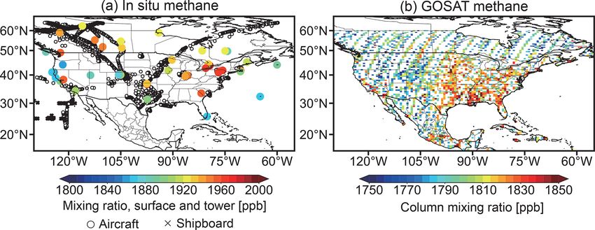
402                                                   X. Lu et al.: Methane emissions in the United States, Canada, and Mexico

Figure 2. Prior estimates of methane emissions from individual sectors. Anthropogenic emissions are from spatially explicit versions of
the EPA, ECCC, and INECC official national inventories. Wetland emissions are from the mean of the high-performance subset of the
WetCHARTs inventory ensemble.

The posterior error covariance and averaging kernel matri-             et al. (2021). A GEOS-Chem simulation with prior emis-
ces Ŝ0 and A0 on the log solution are obtained by replacing           sion estimates yields a prior model estimate F(x A ) of con-
SA and K with S0A and K0 in Eqs. (3) and (4). Optimization             centrations at the observation points. The mean 2010–2017
of emissions in log space means that x̂ 0 is a best estimate           discrepancy between the observations and the prior model,
of the median of the lognormal error distribution rather than          y − F(x A ), is determined for each grid cell (for GOSAT), in-
the mean. The mean values for spatial and sectoral aggrega-            dividual observation site (surface and tower), and observa-
tion purposes can be inferred from the properties of the log-          tion platform (shipboard and aircraft). y − F(x A ) is taken to
                                                  0
normal distribution as xj (mean) = xj (median) eŝjj /2 , where ŝjj
                                                                  0    represent the systematic bias in the prior emissions to be cor-
is the corresponding diagonal element of the posterior error           rected in the inversion. The residual term, εO = y − F(x A ) −
covariance matrix in log space, i.e., the geometric error stan-        y − F(x A ), represents the random observation error includ-
dard deviation. The boundary conditions are still optimized            ing contributions from the measurements, the forward model,
with normal error distributions, assuming an error standard            and the representation of the observation points on the model
deviation of 10 ppb.                                                   grid (Heald et al., 2004). The variance of εO provides the
   The above describes our base inversion. We also conduct             diagonal terms of SO . The resulting observation error stan-
sensitivity inversions using different error assumptions. This         dard deviations average 13 ppb for GOSAT, 26 ppb for sur-
includes (1) using the quadrature sum of error variances for           face sites, 39 ppb for towers, 19 ppb for ships, and 22 ppb
all sectors contributing to a given Gaussian with a cap of             for aircraft. The observation error is larger for in situ than
50 % following Maasakkers et al. (2021), resulting in a 43 %           for satellite observations, even though the in situ measure-
error on average; (2)–(4) using the normal error distributions         ments are more precise, because the forward model error is
(then with the linear Jacobian matrix) with 50 %, 95 %, and            larger for vertically resolved points (particularly for surface
the quadrature sum of errors for individual Gaussians as er-           air in source regions) than for atmospheric columns (Cus-
ror variances; and (5) assuming an error standard deviation            worth et al., 2018). The observation error for in situ observa-
of 5 ppb for boundary conditions.                                      tions is dominated by the forward model error, while that for
   The observation error covariance matrix SO includes con-            GOSAT is dominated by the measurement error.
tributions from measurement and forward model errors. We                  We do not have sufficient objective information to quan-
compute it following the residual error method originally de-          tify the error correlation structure of SO , and we therefore
scribed by Heald et al. (2004) and previously used by Lu               assume it to be diagonal. This may underestimate SO be-

Atmos. Chem. Phys., 22, 395–418, 2022                                                    https://doi.org/10.5194/acp-22-395-2022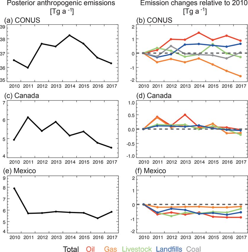
X. Lu et al.: Methane emissions in the United States, Canada, and Mexico                                                                 403

cause of correlated transport and source aggregation errors         Following Shen et al. (2021), fi is then given by
in the forward model, as noted above. We follow Zhang
et al. (2018) to introduce a regularization factor γ for the                   ηαi σi2 (1 − f0 )
                                                                    fi = 1 −                       ,                                      (8)
observation terms in the cost function J (x) (Eq. 1) to avoid                           σA2
either overfits or underfits that would result from missing co-
variant (off-diagonal) structure in SO and SA , respectively.       where αi is the fraction of total emissions in the grid cell
Lu et al. (2021) showed that the optimal value of this reg-         contributed by sector i, σA is the prior error standard devia-
                                                                                                                             σA2
ularization factor can be selected such that the sum of the         tion for total emissions in the grid cell, and η =   q               is a
                                                                                                                               αi2 σi2
                                                                                                                         P
n prior terms in the posterior estimate of the cost function                                                             i=1
(JA (x̂) = (x̂ − x A )T S−1
                         A (x̂ − x A )) has a value ≈ n,which is    normalization factor. For the prior error standard deviations
the expected value from the chi-square distribution with n          σi on the 0.5◦ ×0.625◦ grid we use the scale-dependent adap-
degrees of freedom. Here we determine the regularization            tation by Maasakkers et al. (2016) of EPA sectoral national
factor γ separately for in situ and GOSAT data following            error estimates. This results in prior error standard deviations
Lu et al. (2021) and find that γ = 1 is best for both. We also      of 43 % for rice, 66 % for wastewater, 51 % for landfills, 38 %
conduct a sensitivity inversion using γ = 0.5 for the GOSAT         for livestock, 18 % for coal, 30 % for gas, and 87 % for oil
observation terms (while keeping γ = 1 for in situ data terms       emissions. We further use 70 % for wetlands (Bloom et al.,
in the joint inversion) as adopted in Maasakkers et al. (2021).     2017) and 100 % for all other natural sources. These error
   Table 2 summarizes the settings of our base inversion (in        estimates are solely used to infer fi values in Eq. (8) so that
bold) and the inversion ensemble. The ensemble comprises            more uncertain emissions will contribute more to the correc-
33 inversions using the different combinations of settings in       tion. We use the second method in our base attribution of
the table. The base inversion including GOSAT and in situ           posterior estimates to emission sectors but will also use the
data represents our best estimate, but we will compare it           results from the first method to contribute to error ranges in
prominently to the GOSAT-only and in-situ-only inversions           these sector-attributed posterior estimates.
with the same inversion parameters in order to evaluate the            We also need to aggregate posterior emission estimates na-
contributions from the different observing platforms for op-        tionally and by sector for comparison to the national emis-
timizing emissions. We will use the other ensemble members          sion inventories. Following Maasakkers et al. (2019), this is
to discuss the sensitivity of inversion results to the choices of   done by a transformation from the posterior full-dimension
observations and inversion parameters, as well as to define         state vector x̂ to the reduced state vector x̂ red (national emis-
the range of uncertainty in the inversion results.                  sion for a given sector) with a summation matrix W:

                                                                    x̂ red = Wx̂.                                                         (9)
2.6   Sectoral attribution and aggregation of inversion               The posterior error covariance and averaging kernel matri-
      results                                                       ces for the reduced state vector are then given by
The inversion returns the posterior estimates of mean emis-         Ŝred = WŜWT ,                                                      (10)
sions for each of the Gaussians, and we allocate these emis-        Ared = WAW ,    ∗
                                                                                                                                         (11)
sions to the native 0.5◦ × 0.625◦ model grid by summing
the contributions of all Gaussians on the grid. This de-            where W∗ = WT (W WT )−1 (Calisesi et al., 2005). Ŝred en-
fines a correction factor f0 to total prior emissions for each      ables us to determine whether national correction factors for
0.5◦ × 0.625◦ grid cell and including the contributions from        individual sectors are affected by error correlations between
all q emission sectors (in our case q = 12; see Table 1). For       sectors. Ared enables us to determine the ability of the ob-
sectoral attribution of this total correction factor we need        serving system to quantify national emissions from a partic-
to derive the correction factors fi to the individual sectors       ular sector independently from the prior estimate.
i ∈ [1, q] contributing to f0 .
   We use two alternative methods for this purpose. The first
                                                                    3     Results and discussion
method simply takes fi = f0 for all i, thus assuming that
the partitioning of sectoral emissions in individual grid cells
                                                                    3.1    Base inversion compared to GOSAT-only and
is correct in the prior inventory and all sectors contribute
                                                                           in-situ-only inversions
equally to the grid-level correction factor (Maasakkers et al.,
2021; Lu et al., 2021; Zhang et al., 2021). These assump-           Figure 3a shows the gridded posterior correction factors from
tions are reasonable when the sectors are spatially separated       the base inversion averaged over 2010–2017, i.e., the mul-
but may be a source of error when they spatially overlap.           tiplicative factors applied to the total prior emissions from
The second method (Shen et al., 2021) accounts for emis-            Fig. 2, mapped on the 0.5◦ × 0.625◦ model grid. Figure 3b
sions from different sectors having different prior error stan-     shows the corresponding averaging kernel sensitivities, indi-
dard deviation σi and therefore contributing differently to f0 .    cating the dependence of the posterior solution on the prior

https://doi.org/10.5194/acp-22-395-2022                                                   Atmos. Chem. Phys., 22, 395–418, 2022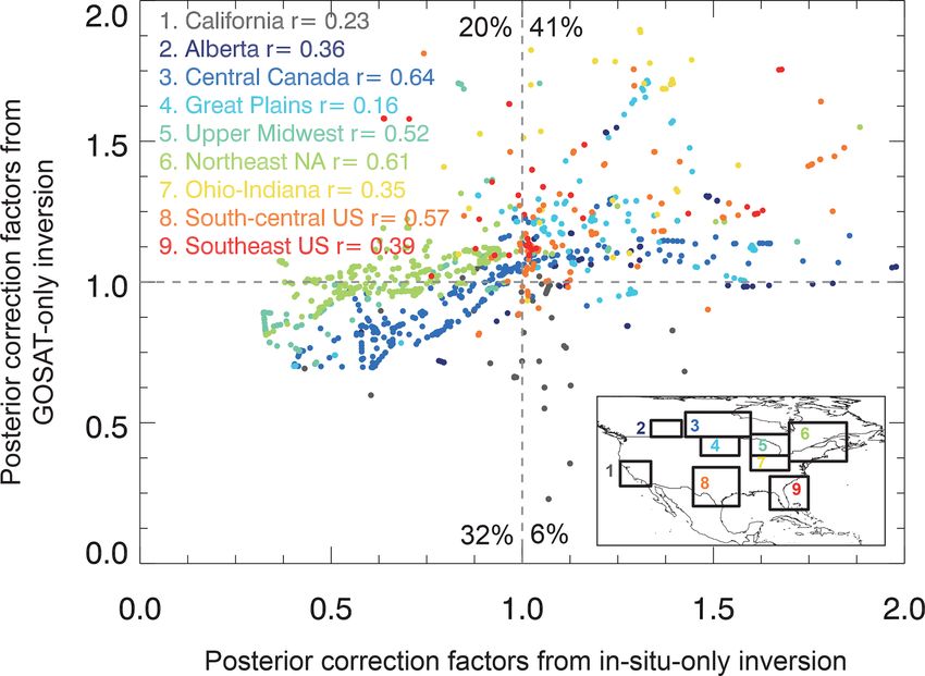
404                                                                X. Lu et al.: Methane emissions in the United States, Canada, and Mexico

Table 2. Settings for generation of the 33-member inversion ensemblea .

           Observations                               Regularization parameter γ                               Prior error standard deviation
                                                                                               Emissions                            Boundary conditions
           GOSAT + in situ                            1                                        50 % (lognormal)                          10 ppb
           GOSAT + in situ (long-term)c               0.5 (GOSAT)                              quadrature sum (lognormal)d               5 ppb
           GOSAT                                                                               50 % (normal)
           In situ                                                                             95 % (normal)
           In situ (long-term)c                                                                quadrature sum (normal)d
         a Settings for the base inversion are in bold. The 33-member inversion ensemble uses the different combinations of settings to probe the effects of different
         choices in observations and in inversion parameters. The GOSAT + in situ inversion includes the following seven-member ensemble: (1) base inversion with
         γ = 1 for in situ and GOSAT observations , σA = 50 % (lognormal) for emissions, and σA = 10 ppb for boundary conditions; (2) the same as (1) except that
         γ = 0.5 for GOSAT observations; (3)–(6) the same as (1), except that σA for emissions uses the other four options in the table; and (7) is the same as (1),
         except that σA = 5 ppb for boundary conditions. Similarly, the GOSAT + in situ (long-term) and GOSAT inversions have seven ensemble members,
         respectively. The in situ and in situ (long-term) inversions have six ensemble members, respectively. This adds up to 33 inversion ensemble members.
         Sectoral attribution is done by two alternative methods (see text in Sect. 2.6), resulting in a total of 66 members.
         c Including only long-term surface and tower sites with observations for all years of the 2010–2017 record.
         d Adding the errors from individual sectors in quadrature following Maasakkers et al. (2021).

estimate (0: total dependence, 1: no dependence). The num-                                 overall good consistency between the two inversions (cor-
ber of independent pieces of information afforded by the ob-                               relation coefficient r = 0.47 for the ensemble of points, with
servations (DOFS = 114) can be placed in the context of the                                73 % of grid cells showing corrections in the same direction).
600 Gaussian state vector elements used to optimize the spa-                               The reduced-major-axis regression slope is 0.62, consistent
tial distribution of emissions. We see that the observations                               with GOSAT providing overall less information. Both inver-
provide considerable information to optimize methane emis-                                 sions find that methane emissions over the south-central US,
sions, but we also see that a finer resolution for the inversion                           the southeast US, the Great Plains, and Alberta are underes-
would not be justified on the continental scale.                                           timated in the prior inventories. They also agree on down-
   Figure 3c–f show the results from the GOSAT-only and in-                                ward corrections over central Canada and the upper Mid-
situ-only inversions, enabling us to compare the information                               west where wetland emissions dominate. The largest incon-
contents and consistency of the two data sets. The GOSAT-                                  sistency is over California where the two inversions show
only inversion yields a DOFS of 68, while the in-situ-only                                 correction factors in the opposite direction for much of the
inversion yields a DOFS of 80, even though there are 50 %                                  state. This may reflect the coarse resolution of model CO2
fewer in situ observations than GOSAT observations. This is                                used in the proxy GOSAT retrieval that leads to underesti-
because the sensitivities of surface observations to emissions                             mation of CO2 (and hence methane) over the Los Angeles
are an order of magnitude higher than those of satellite ob-                               Basin (Turner et al., 2015; Maasakkers et al., 2021) and/or
servations (Cusworth et al., 2018). The GOSAT observations                                 complex topography. Results from the base inversion tend
have the advantage of broader coverage. Thus, we find that                                 toward either of the two inversions depending on which has
the in situ observations dominate the information content of                               the most information content.
the base inversion over California, the upper Midwest, and                                    We evaluated the ability of the base GOSAT + in situ in-
Canada, whereas GOSAT dominates the information con-                                       version to fit the two observational data sets by comparing
tent in Mexico (where there are no in situ observations) and                               2010–2017 GEOS-Chem simulations with posterior versus
most of the western US. GOSAT and in situ observations                                     prior emissions and boundary conditions. Results are shown
contribute comparably in the south-central and eastern US,                                 in Fig. 5. The posterior simulation reduces the model mean
though with different weights in different locations. We con-                              bias (MB) in surface and tower measurements from −11 ppb
clude that GOSAT and in situ observations make compara-                                    in the prior simulation to −5 ppb, and it also narrows the root
ble and complementary contributions to the optimization of                                 mean square error (RMSE) from 24 to 14 ppb. For GOSAT
methane emissions for North America.                                                       the improvement is less apparent from the continental-scale
   We next examine the consistency in the information from                                 comparison statistics because the prior simulation already
GOSAT and in situ observations for correcting prior methane                                has a low mean bias (MB = −0.5 ppb) and a small RMSE
emissions. Inspection of the posterior correction factors from                             of 6.9 ppb. However, we see from Fig. 5 that the small
the GOSAT-only and in-situ-only inversions in Fig. 3 shows                                 mean bias reflects an offset between high bias in the west-
overall qualitative agreement. Figure 4 displays a more quan-                              ern US and Canada and low bias in the central and eastern
titative comparison of the posterior corrections by correlating                            US. The inversion results in spatial whitening of this bias.
the values for 0.5◦ × 0.625◦ grid cells between the GOSAT-                                 Independent evaluation with the ground-based column ob-
only and in-situ-only inversions, selecting regions with rel-                              servations from the Total Carbon Column Observing Net-
atively high averaging kernel sensitivities for both. We find                              work (TCCON) (Wunch et al., 2011) further shows that the

Atmos. Chem. Phys., 22, 395–418, 2022                                                                                https://doi.org/10.5194/acp-22-395-2022
X. Lu et al.: Methane emissions in the United States, Canada, and Mexico 405
Figure 3. Optimization of mean 2010–2017 methane emissions over North America. Results are from the base inversion using both GOSAT
and GLOBALVIEWplus in situ observations, the GOSAT-only inversion, and the in-situ-only inversion. The left panels show the posterior
correction factors, i.e., the multiplicative factors applied to the total prior emissions in Fig. 2, and the right panels show the averaging
kernel sensitivities (diagonal elements of the averaging kernel matrix). The degrees of freedom for signal (DOFS, defined as the trace of the
averaging kernel matrix) are shown in the inset.
mean model bias at five sites in CONUS decreases from 5.2– ance matrix (Eq. 10) to evaluate the ability of the inversion
14.0 ppbv in the prior simulation to 1.0–13.5 ppbv in the pos- to separate between sectors. This is shown in Fig. 6 as the
terior simulation. posterior error correlation matrix, displaying the error cor-
relation coefficients (r) in the inversion results for all sec-
3.2 Optimized 2010–2017 anthropogenic methane tor pairs. Error correlation coefficients are generally lower
emissions for CONUS, Canada, and Mexico than 0.2 for CONUS, indicating successful separation, except
for small sources (termites, seeps, other anthropogenic). The
Table 1 (a–c) summarizes our inversion results for na- same holds for Canada except for error correlation between
tional 2010–2017 methane emissions by sector in CONUS, landfills and wastewater treatment, which are both associated
Canada, and Mexico. Our best posterior estimates of to- with urban areas. Anthropogenic emissions in Canada are
tal anthropogenic + natural emissions from the base inver- well separated from the large wetland emissions. Error cor-
sion are 46.3 (40.2–48.4) Tg a−1 for CONUS, 16.2 (13.5– relations are higher in Mexico because emissions from dif-
17.4) Tg a−1 for Canada, and 6.8 (5.4–6.9) Tg a−1 for Mex- ferent sectors tend to be concentrated in Mexico City and the
ico. The ranges given in parentheses are from the 33 inver- eastern part of the country (Scarpelli et al., 2020), but even
sion ensemble members (Table 2). Averaging kernel sensitiv- there the error correlation coefficients are generally less than
ities for these total national emissions (the diagonal elements 0.4. Optimization of the oil and gas sector is well separated
in Ared , Sect. 2.6) are 0.72 for CONUS, 0.60 for Canada, and from the other sectors in all three countries, and separation
0.40 for Mexico, indicating that the GOSAT + in situ obser- between oil and gas is also successful because the two sec-
vation system informs 72 % of total methane emissions in tors have very different spatial distributions in the gridded in-
CONUS, 60 % in Canada, and 40 % in Mexico, with the re- ventories (Fig. 2). However, there is some ambiguity for the
mainder of the posterior emissions anchored to the prior es- production subsectors because wells often produce both oil
timate. The lower information content for Mexico is due to and gas (Maasakkers et al., 2016), and for this reason some
the lack of in situ observations. studies prefer to refer to oil and gas emissions as a combined
We partition these national totals into different sectors as sector (Alvarez et al., 2018). Separating oil and gas emis-
described in Sect. 2.6 and use the posterior error covari-
https://doi.org/10.5194/acp-22-395-2022 Atmos. Chem. Phys., 22, 395–418, 2022406 X. Lu et al.: Methane emissions in the United States, Canada, and Mexico
Figure 4. Comparison of posterior correction factors to prior methane emissions on the 0.5◦ × 0.625◦ grid between GOSAT-only and in-
situ-only inversions. The comparisons are for nine regions with relatively high averaging kernel sensitivities for both inversions. Each point
represents the posterior correction factors from both inversions in a 0.5◦ × 0.625◦ grid cell (Fig. 3). Correlation coefficients for each of the
nine regions are shown in the inset. Percentiles in each quadrant show the fraction of the total points in that quadrant.
sions is useful for our purpose because such separation is of 6.1 Tg a−1 for Canada by inversion of data from GOSAT
required under UNFCCC reporting, but the reader should be and ECCC surface sites.
aware that this separation is done on the basis of the spatial Our best estimate of the mean 2010–2017 anthropogenic
distributions of emissions in Fig. 2. methane emission for Mexico is 6.0 (4.7–6.1) Tg a−1 , which
We find that anthropogenic methane emissions for all three is 20 % higher than the 5.0 Tg a−1 in Mexico’s national in-
countries are larger in our inversion results than in the na- ventory (INECC and SEMARNAT, 2018) used as a prior es-
tional inventories submitted to the UNFCCC. Our best esti- timate. Shen et al. (2021) similarly found higher emissions
mate of the mean 2010–2017 anthropogenic methane emis- than the national inventory in their inversion of TROPOMI
sion for CONUS is 36.9 (32.5–37.8) Tg a−1 , which is 30 % satellite methane data for eastern Mexico.
higher than the 28.7 Tg a−1 in the 2016 version of the EPA Figure 7 displays the data from Table 1a–c for the na-
GHGI used as a prior estimate (EPA, 2016) and 42 % higher tional posterior emission estimates from different sectors in
than the mean 26.0 Tg a−1 for 2010–2017 in the most recent comparison with the EPA (US), ECCC (Canada), and IN-
version of the GHGI (EPA, 2021). Maasakkers et al. (2021) ECC (Mexico) national inventories used as prior estimates.
previously obtained a mean 2010–2015 CONUS anthro- We find that emissions from all major sectors except coal
pogenic emission of 30.6 (29.4–31.3) Tg a−1 by inversion of and wastewater are lower in the national inventories than our
GOSAT data using the same prior anthropogenic estimate as inversion results, with the largest underestimates for fugi-
ours but a much higher prior estimate for CONUS wetlands tive emissions from the oil sector. The total CONUS oil and
(15.7 Tg a−1 ). The need to decrease the wetlands source in gas emissions in our inversion are 4.6 and 9.9 Tg a−1 , re-
their inversion (to a posterior estimate of 11.8 Tg a−1 ), as spectively, which is 109 % and 45 % higher than the EPA
well as their reliance on GOSAT observations only, may have (2016) inventory used here as a prior estimate and 177 % and
dampened their ability to quantify anthropogenic emissions. 65 % higher than the most recent EPA (EPA, 2021) inventory
Our best estimate of the mean 2010–2017 anthropogenic for the 2010–2017 mean. The EPA inventory reports an un-
methane emission for Canada is 5.3 (3.6–5.7) Tg a−1 , which certainty of −24 % to +29 % for oil and −15 % to +14 %
is 43 % higher than the 3.7 Tg a−1 in the ECCC NIR (2020 for natural gas emissions (EPA, 2021). Our estimates are
version) used as a prior estimate and 33 % higher than the also higher than those in Maasakkers et al. (2021), which
4.0 Tg a−1 for 2010–2017 reported in the most recent version are 3.6 and 8.0 Tg a−1 , respectively, for oil and gas emis-
of the ECCC NIR (ECCC, 2021). Baray et al. (2021) previ- sions in 2010–2015. They are consistent with the Alvarez
ously obtained a mean 2010–2015 anthropogenic emission et al. (2018) estimates for total CONUS oil and gas emis-
sions of 13 (11–15) Tg a−1 in 2015 based on field measure-
Atmos. Chem. Phys., 22, 395–418, 2022 https://doi.org/10.5194/acp-22-395-2022X. Lu et al.: Methane emissions in the United States, Canada, and Mexico 407 Figure 5. Ability of the base inversion to fit the in situ (surface and tower) and GOSAT observations for 2010–2017. The figure shows the mean differences between GEOS-Chem simulations and the observations using either prior or posterior methane emissions. Mean bias (MB) and root mean square error (RMSE) are shown in the inset, calculated from the temporally averaged differences for each in situ site or GOSAT grid cell. ments within oil and gas basins, scaled up to derive a national 2017 surface methane measurements in western Canada value. (Chan et al., 2020). Most of the information for Canada in We mentioned previously that the lower estimates in our base inversion indeed comes from the in situ measure- Maasakkers et al. (2021) could reflect their use of GOSAT ments (Fig. 3), which are relatively dense in Canada (Fig. 1), observations only, the difference in time frame, and their and considering that GOSAT observations at high latitudes high prior estimate for wetlands, but another factor is their are relatively sparse and seasonally limited (Lu et al., 2021). assumption of normal distributions for prior emission error Maasakkers et al. (2021) previously found little information standard deviations. We find from our inversion ensemble for Canadian anthropogenic emissions in their GOSAT-only that assuming a lognormal distribution (as in our base inver- inversion, although that was further complicated by their sion) rather than a normal distribution increases the resulting large overestimate of prior wetland emissions that dominate posterior oil and gas emissions by 0.8 and 0.9 Tg a−1 , respec- total emissions in Canada. tively. This is because the lognormal distribution does much We further compared our oil and gas inversion results for better at capturing the heavy tail of the emission probability CONUS, Canada, and Mexico to the TRACE bottom-up in- density functions for oil and gas production (Zavala-Araiza ventory aggregating data from individual assets up to the et al., 2015; Frankenberg et al., 2016; Alvarez et al., 2018). country level (Climate TRACE, 2021). This inventory uses Adding the in situ observations to the GOSAT-only inversion life-cycle assessment emissions models for production, pro- further increases the posterior oil and gas emissions by 0.2 cessing, refining, and shipping (Gordon et al., 2015; Mas- and 0.3 Tg a−1 , respectively. The assumption of larger un- nadi et al., 2018; Gordon and Reuland, 2021). The TRACE certainty of oil than gas emissions in Eq. (8) furthermore oil and gas total emission estimates for CONUS (9.6 Tg a−1 ), attributes larger upward corrections to oil emissions. Thus, Canada (1.8 Tg a−1 ), and Mexico (0.8 Tg a−1 ) are similar to our base inversion yields the high end of the estimated range the prior estimates from the EPA, ECCC, and INECC, re- from the inversion ensemble (Table 1a) but still represents spectively (Table 1), and correspondingly lower than our best our best estimate. posterior estimates of 14.5 Tg a−1 for CONUS, 3.2 Tg a−1 for Our inversion increases the oil emissions over Canada Canada, and 1.3 Tg a−1 for Mexico. The bottom-up oil and by more than a factor of 2 to 1.8 Tg a−1 compared to the gas modeling in TRACE assesses routine methane emissions ECCC inventory. The total posterior oil and gas emissions for from normal operations, assuming normal fugitive emis- Canada are 2.9 (1.6–3.3) Tg a−1 . This is in good agreement sions. Recent flyover work, however, shows that methane with a recent inversion study (3.0 Tg a−1 ) based on 2010– https://doi.org/10.5194/acp-22-395-2022 Atmos. Chem. Phys., 22, 395–418, 2022
You can also read