Modeling and mitigation of cross-talk effects in readout noise with applications to the Quantum Approximate Optimization Algorithm
←
→
Page content transcription
If your browser does not render page correctly, please read the page content below

Modeling and mitigation of cross-talk effects in readout noise
                                            with applications to the Quantum Approximate Optimization
                                            Algorithm
                                            Filip B. Maciejewski1 , Flavio Baccari2 , Zoltán Zimborás3,4,5 , and Michał Oszmaniec1

                                            1
                                                Center for Theoretical Physics, Polish Academy of Sciences, Al. Lotników 32/46, 02-668 Warsaw, Poland
                                            2
                                                Max-Planck-Institut für Quantenoptik, Hans-Kopfermann-Straße 1, 85748 Garching, Germany
                                            3
                                                Wigner Research Centre for Physics, H-1525 Budapest, P.O.Box 49, Hungary
                                            4
                                                BME-MTA Lendület Quantum Information Theory Research Group, Budapest, Hungary
                                            5
                                                Mathematical Institute, Budapest University of Technology and Economics, P.O.Box 91, H-1111, Budapest, Hungary
arXiv:2101.02331v3 [quant-ph] 27 May 2021

                                                        Measurement noise is one of the main sources of errors in currently available quantum
                                                    devices based on superconducting qubits. At the same time, the complexity of its charac-
                                                    terization and mitigation often exhibits exponential scaling with the system size. In this
                                                    work, we introduce a correlated measurement noise model that can be efficiently described
                                                    and characterized, and which admits effective noise-mitigation on the level of marginal prob-
                                                    ability distributions. Noise mitigation can be performed up to some error for which we derive
                                                    upper bounds. Characterization of the model is done efficiently using Diagonal Detector
                                                    Overlapping Tomography – a generalization of the recently introduced Quantum Overlap-
                                                    ping Tomography to the problem of reconstruction of readout noise with restricted locality.
                                                    The procedure allows to characterize k-local measurement cross-talk on N -qubit device using
                                                    O k2k log (N ) circuits containing random combinations of X and identity gates. We perform
                                                    experiments on 15 (23) qubits using IBM’s (Rigetti’s) devices to test both the noise model and
                                                    the error-mitigation scheme, and obtain an average reduction of errors by a factor > 22 (> 5.5)
                                                    compared to no mitigation. Interestingly, we find that correlations in the measurement noise
                                                    do not correspond to the physical layout of the device. Furthermore, we study numerically
                                                    the effects of readout noise on the performance of the Quantum Approximate Optimization
                                                    Algorithm (QAOA). We observe in simulations that for numerous objective Hamiltonians,
                                                    including random MAX-2-SAT instances and the Sherrington-Kirkpatrick model, the noise-
                                                    mitigation improves the quality of the optimization. Finally, we provide arguments why in
                                                    the course of QAOA optimization the estimates of the local energy (or cost) terms often
                                                    behave like uncorrelated variables, which greatly reduces sampling complexity of the energy
                                                    estimation compared to the pessimistic error analysis. We also show that similar effects are
                                                    expected for Haar-random quantum states and states generated by shallow-depth random
                                                    circuits.

                                            1 Introduction                                                   fully functional quantum devices. With state of
                                                                                                             the art quantum processors reaching a scale of
                                            1.1 Motivation                                                   50-100 qubits [1], the scientific community is ap-
                                                                                                             proaching a regime in which quantum systems
                                            Outstanding progress has been made in the last
                                                                                                             cannot be modeled on modern supercomputers
                                            years on the path to development of scalable and
                                                                                                             using known methods [2]. This situation is unar-
                                            Filip B. Maciejewski: filip.b.maciejewski@gmail.com              guably exciting since it opens possibilities for the
                                            Michał Oszmaniec: oszmaniec@cft.edu.pl                           first demonstrations of quantum advantage and,

                                            Accepted in    Quantum 2021-05-18, click title to verify. Published under CC-BY 4.0.                                 1
potentially, useful applications [3–5]. At the same             estimation of the local terms (which can be per-
time, however, it entails a plethora of non-trivial             formed simultaneously). Since the estimation of
problems related to fighting effects of experimen-              marginal distributions is the task of low sam-
tal imperfections on the performance of quantum                 pling and post-processing complexity, this sug-
algorithms. As quantum devices in the near-term                 gests that error mitigation techniques can be effi-
will be unable to implement proper error cor-                   ciently applied in QAOA. In this work, we present
rection [5], various methods of noise mitigation                a number of contributions justifying the usage of
have been recently developed [6–15]. Those meth-                measurement error-mitigation in QAOA, even in
ods aim at reducing the effects of errors present               the presence of significant cross-talk effects.
in quantum gates and/or in quantum measure-
ments. In this work, we focus on the latter, i.e.,              1.2 Results outline
noise affecting quantum detectors.
                                                                Our first contribution is to provide an efficiently
   Indeed, it has been found in currently available             describable measurement noise model that in-
quantum devices that the noise affecting mea-                   corporates asymmetric errors and cross-talk ef-
surements is quite significant. Specifically, errors            fects. Importantly, our noise model admits ef-
of the order of a few percent in a single qubit                 ficient error-mitigation on the marginal proba-
measurement and non-negligible effects of cross-                bility distributions, which can be used, e.g., for
talk were reported [1, 13–16]. Motivated by this,               improvement of the performance of variational
a number of methods to characterize and/or re-                  quantum algorithms. We show how to efficiently
duce measurement errors were proposed [13–23].                  characterize the noise using a number of circuits
Readout noise mitigation usually relies on the                  scaling logarithmically with the number of qubits.
classical post-processing of experimental statis-               To this aim, we generalize the techniques of the
tics, preceded by some procedure of noise char-                 recently introduced Quantum Overlapping To-
acterization. Existing techniques typically suf-                mography (QOT) [33] to the problem of readout
fer from the curse of dimensionality due to char-               noise reconstruction. Specifically, we introduce
acterization cost, sampling complexity, and the                 notion of Diagonal Detector Overlapping Tomog-
complexity of post-processing – which scale ex-                 raphy (DDOT) which allows to reconstruct noise
ponentially with the number of qubits N . For-                                 k-local cross-talk
                                                                description with                   on N -qubit de-
                                                                                  k
                                                                vice using O k2 log (N ) quantum circuits con-
tunately, some interesting problems in quantum
computing do not require measurements to be                     sisting of single layer of X and identity gates.
performed across the whole system. An impor-                    Furthermore, we explain how to use that charac-
tant class of algorithms that have this feature are             terization to mitigate noise on the marginal dis-
the Quantum Approximate Optimization Algo-                      tributions and provide a bound for the accuracy
rithms (QAOA) [24], which only require the es-                  of the mitigation. Importantly, assuming that
timation of a number of few-particle marginals.                 cross-talk in readout noise is of bounded local-
QAOA is a heuristic, hybrid quantum-classical                   ity, the sampling complexity of error-mitigation
optimization technique [24, 25], that was later                 is not significantly higher than that of the start-
generalized as a standalone ansatz [26] shown                   ing problem of marginals estimation.
to be computationally universal [27, 28]. In its                   We test our error-mitigation method in exper-
original form, QAOA aims at finding approxi-                    iments on 15 qubits using IBM’s device and on
mate solutions for hard combinatorial problems,                 23 qubits using Rigetti’s device, both architec-
notable examples of which are maximum satis-                    tures based on superconducting transmon qubits
fiability (SAT) [29], maximum cut (MAXCUT)                      [34]. We obtain a significant advantage by using a
[30], or the Sherrington-Kirkpatrick (SK) spin-                 correlated error model for error mitigation in the
glass model [31, 32]. Regardless of the underly-                task of ground state energy estimation. Interest-
ing problem, the main QAOA subroutine is the                    ingly, the locality structure of the reconstructed
estimation of the energy of the local classical                 errors in these devices does not match the spatial
Hamiltonians on a quantum state generated by                    locality of qubits in these systems.
the device. Those Hamiltonians are composed of                     We also study statistical errors that appear
a number of a few-body commuting operators,                     in the simultaneous estimation of multiple lo-
and hence estimation of energy can be done via                  cal Hamiltonian terms that appear frequently in

Accepted in   Quantum 2021-05-18, click title to verify. Published under CC-BY 4.0.                              2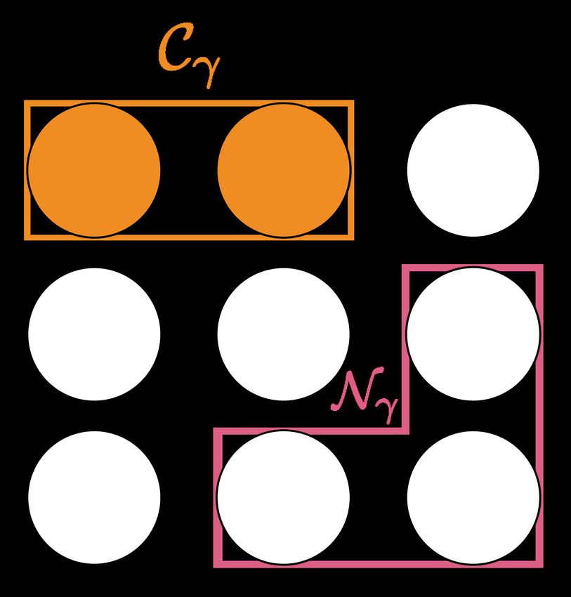
QAOAs. In particular, we provide arguments                         Alternative methods of characterization of cor-
why one can expect that the estimated energies of               related measurement noise were recently pro-
local terms behave effectively behave as uncorre-               posed in Refs. [15, 16, 20]. Out of the above-
lated variables, for the quantum states appearing               mentioned works, perhaps the most related to
at the beginning and near the end of the QAOA                   ours in terms of studied problems is Ref. [15],
algorithm. This allows to prove significant re-                 therefore we will now comment on it thoroughly.
ductions in sampling complexity of the total en-                The authors introduced a correlated readout
ergy estimation (compared to the worst-case up-                 noise model based on Continuous Time Markov
per bounds).                                                    Processes (CTMP). They provide both error-
   Finally, we present a numerical study and de-                characterization and error-mitigation methods.
tailed discussion of the possible effects that mea-             The CTMP noise model assumes that the noisy
surement noise can have on the performance of                   stochastic process in a measurement device can
the Quantum Approximate Optimization Algo-                      described by a set of two-qubit generators with
rithm. This includes the study of how noise                     corresponding error rate parameters. The to-
distorts the quantum-classical optimization in                  tal number of parameters required to describe
QAOAs. We simulate the QAOA protocol on                         a generic form of such noise for N -qubit device
an 8-qubit system affected by correlated mea-                   is 2N 2 . The authors propose a method of noise
surement noise inspired by the results of IBM’s                 characterization that requires preparation of a set
device characterization. For a number of ran-                   of suitably chosen classical states and perform-
dom Hamiltonians, we conclude that the error-                   ing a post-selection on the noise-free outcomes
mitigation highly improves the accuracy of energy               (i.e., correct outcomes given known input classi-
estimates, and can help the optimizer to converge               cal state) on the subset of (N − 2) qubits. Since
faster than when no error-mitigation is used.                   probability of noise-free outcomes can be expo-
                                                                nentially small even for the uncorrelated read-
1.3 Related works                                               out noise, this method can prove relatively costly
                                                                in practice. We believe that our DDOT char-
The effects of simple, uncorrelated noisy quantum               acterization technique could prove useful in re-
channels on QAOAs were analyzed in Refs. [35–                   ducing the number of parameters needed to de-
37]. In particular, the symmetric bitflip noise an-             scribe CTMP model (by showing which pairs of
alyzed in [35] can be used also to model sym-                   qubits are correlated, and for which the cross-
metric, uncorrelated measurement noise - a type                 talk can be neglected), hence allowing for much
of readout noise which has been demonstrated to                 more efficient version of noise reconstruction pre-
be not very accurate in currently available de-                 sented in Ref. [15]. The authors also present a
vices based on transmon qubits [13, 16]. A simple               novel noise-mitigation method that allows to es-
readout noise-mitigation technique on the level                 timate the noise-reduced expected values of ob-
of marginals for QAOAs was recently experimen-                  servables. The method is based on decomposi-
tally implemented on up to 23 qubits in a work                  tion of inverse noise matrix into the linear com-
by Google AI Quantum team and collaborators                     bination of stochastic matrices, and constructing
[38]. Importantly, the authors assumed uncorre-                 a random variable (with the aid of classical ran-
lated noise on each qubit – we believe that our                 domness and post-processing) that agrees in the
approach which accounts for correlations could                  expected value of noise-free observable. In gen-
prove beneficial in those kinds of experiments.                 eral, both sampling complexity and classical post-
In a similar context, readout noise-mitigation us-              processing cost scale exponentially with the num-
ing classical post-processing on global probabil-               ber of qubits. Since the authors aim to correct
ity distributions was implemented in QAOA and                   observables with arbitrary locality, the problem
Variational Quantum Eigensolver (VQE) experi-                   they consider is different to our approach that
ments on up to 6 qubits [39, 40]. While for such                aims to correct only local observables (and there-
small system sizes it is possible to efficiently per-           fore does not exhibit exponential scalings). It is
form global error mitigation, we emphasize that                 an interesting problem to see whether the CTMP
our approach based on the noise-mitigation on                   noise model can also be interpreted on the level of
the marginals could be performed also in larger                 marginal probability distributions in a way that
experiments of this type.

Accepted in   Quantum 2021-05-18, click title to verify. Published under CC-BY 4.0.                              3
allows for mitigation analogous to ours in terms Such noise is thus equivalent to a stochastic pro-
of complexity. cess, in which an outcome from a perfect device
probabilistically changes to another (possibly er-
roneous) one. Equation (2) suggests a simple way
2 Correlated readout noise model to mitigate errors on the noisy device – via left-
2.1 Preliminaries multiplying the estimated statistics by the inverse
of noise matrix Λ−1 [13, 14]. From stochasticity
In quantum mechanics, the most general mea- of Λ it follows that its inverse does preserve the
surement M that can be performed is represented sum of the elements of probability vectors, how-
by a Positive Operator-Valued Measure (POVM) ever it may introduce some unphysical (i.e., lower
[41]. A POVM M with r outcomes on a d- than 0 or higher than 1) terms in corrected vec-
dimensional Hilbert space is a set of positive- tor. A common practice in such a scenario is to
semidefinite operators that sum up to identity, solve optimization problem
i.e.,
r p = argminq ||q − Λ−1 pnoisy ||22 , (3)
{Mi }ri Mi = 1, (1)
X
M= , ∀i Mi > 0 ,
where minimization goes over all proper probabil-
i=1
ity distributions. This introduces additional er-
where 1 is the identity operator. When one per- rory in the final estimations which can be easily
forms a measurement M on the quantum state ρ, upper-bounded [13].
the probability of obtaining outcome i is given by Before going further, we note that while mul-
Born’s rule: Pr (i|M, ρ) = tr (ρMi ). tiplication by Λ−1 is perhaps the most natural
In quantum computing a perfect measurement (and simple) method to reduce the noise and has
is often modeled as a so-called projective mea- been shown to be useful in practical situations
surement P = {Pi }ri for which the measurement [13, 14], there exist more sophisticated techniques
operators, in addition to the requirements from of noise-mitigation that do not exhibit this prob-
Eq. (1), are also projectors, i.e., ∀i Pi2 = Pi . lem. For example, Iterative Bayesian Unfold-
While non-projective measurements have many ing [18] always returns physical probability vec-
applications in certain quantum information pro- tors. We note that our noise model and noise-
cessing tasks, in this work we are interested in us- mitigation on marginal probability distributions
ing them to model imperfections in measurement (to be introduced in following sections) is consis-
devices. The relationship between an ideal mea- tent with using methods different than Λ−1 cor-
surement P and its noisy implementation M can rection, and we intend to test them in the future.
be modeled by the application of a generic quan- To finish this introduction, we recall that, as
tum channel. Recently it has been experimen- mentioned above, Eq. (2) does not present the
tally demonstrated for superconducting quantum most general model of quantum measurement
devices that in practice those channels, to a good noise. Specifically, coherent errors might occur,
approximation, belong to a restricted class of and reduce the effectiveness of error-mitigation
stochastic maps [13, 14], which we will refer to as (a detailed analysis of this effect was presented in
’classical measurement noise’. In such a model, [13]). However, it was validated experimentally
the relation between M and P is given by some on multiple occasions, that coherent errors in su-
stochastic transformation Λ. Namely, we have perconducting quantum devices are small, and
P
M = ΛP, i.e., Mi = j Λij Pj . Due to the lin- the error-mitigation by classical post-processing
earity of Born’s rule, it follows that probabilities was shown to work very well in few-qubit scenar-
pnoisy from which noisy detector samples are re- ios [13, 14].
lated to the noiseless probabilities pideal via the
same stochastic map, hence [13]
2.2 Correlations in readout noise
noisy ideal
p = Λp . (2)
The size of the matrix Λ scales exponentially with
Specifically, in the convention where probability the number of qubits. Thus, if one wants to es-
vectors are columns, the noise matrix Λ is left- timate such a generic Λ using standard methods,
stochastic, meaning that each of its columns con- both the number of circuits and sampling com-
tains non-negative numbers that sum up to 1. plexity scale exponentially. Indeed, the standard
Accepted in Quantum 2021-05-18, click title to verify. Published under CC-BY 4.0. 4method of reconstructing Λ is to create all the 2n ine some complicated physical process, which re-
computational basis and estimate the resulting sults in the situation in which the noise matrix
probability distributions (which constitute the ΛCχ on cluster Cχ slightly depends on the state
columns of Λ). We refer to such characterization of the qubits in Nχ . To account for that, we in-
as Diagonal Detector Tomography (DDT), since troduce the second basic object of our model –
it probes the diagonal elements of the measure- the neighborhood of the cluster. The neighbor-
ment operators describing the detector. This is hood Nχ of a cluster Cχ is a group of qubits the
restricted version of more general Quantum De- state of which just before the measurement affects
tector Tomography (QDT) [42–45]. slightly the noise matrix acting on the cluster Cχ .
These complexity issues can be circumvented For example, if Cχ contains only a single qubit,
if one assumes some locality structure in the say Q0 , it is possible that due to some effective
measurement errors. For example, in the sim- ferromagnetic-type interaction, the probability of
plest model with completely uncorrelated readout erroneously detecting state “0” of Q0 as “1” rises
noise, the Λ matrix is a simple tensor product of when the neighboring qubit Q1 is in state “1”
single-qubit error matrices ΛQi (compared to when it is in state 0 00 ).
O A notion related to our “neighborhood” has ap-
Λ= Λ Qi (uncorrelated noise). (4) peared in recent literature. Specifically in the
i
context of measurement error characterization,
In this model, we need to estimate only single- ’spectator qubits’ are the qubits that affect mea-
qubit matrices, which renders the complexity surement noise on other qubits [16, 20]. However,
of the problem to be linear in the number of so far this effect was treated rather as an unde-
qubits. However, for contemporary quantum de- sired complication, while here it is an inherent
vices based on superconducting qubits, it was element of the proposed noise model.
demonstrated that such a noise model is not very Now we are ready to provide an efficient noise
accurate due to the cross-talk effects [1, 13, 14, model. We construct a global noise matrix Λ with
16]. At the same time, the completely correlated matrix elements of the following form
noise is not realistic as well, which motivates the
Y YNχ
search for a model that can account for correla- ΛX1 ...XN |Y1 ...YN = Λ XC . (5)
χ |YCχ
tions in readout errors while still giving an effi- χ
cient description of Λ.
In this work, we propose such a model and give In the next subsection we give some illustrative
a method to characterize it. Let us lay out the examples, but first let us thoroughly describe the
basic concepts of our model. Consider the cor- notation used in the above equation. A collec-
related errors between some group of qubits Cχ . tion {Cχ }χ gives us the partitioning of the set of
The most general way of describing those errors all qubits. Explicitly, Cχ ∩ Cχ0 = ∅ if χ 6= χ0 and
is to treat the qubits in Cχ as a single object, i.e., ∪χ Cχ = [N ], where N is the number of qubits. To
to always consider their measurement outcomes each cluster Cχ the model associate its neighbor-
together. In terms of the noise matrix descrip- hood Nχ . Equation (5) can be now understood
tion, this means that the noise matrix on Cχ is in the following way. The noise matrix ΛYNχ de-
some generic ΛCχ acting on Cχ . This gives rise scribing the measurement noise occurring in clus-
to the first basic object in our model – the clus- ter Cχ depends on the state just before measure-
ters of qubits. The cluster Cχ is a group of qubits ment of the qubits in the neighborhood Nχ of
with correlations between them so strong, that that cluster (hence the superscript YNχ denot-
one can not consider outcomes of their measure- ing that state). Importantly, each ΛYNχ is left-
ments separately. At the same time, it is unlikely stochastic for any state of the neighbors. By XCχ
that in actual devices the correlations between (or YCχ ) we denote bit-strings of qubits belong-
all the qubits will be so strong that one should ing to cluster Cχ which were measured (or put
assign them all to a single cluster. This moti- inside the device just before measurement). Fi-
vates the introduction of another, milder possibil- nally, YNχ indicates the bit-string denoting the
ity. Consider a measurement performed on qubits state just before the measurement of the qubits
in cluster Cχ and some other qubits Nχ (not be- from the neighborhood Nχ of the cluster Cχ (see
ing in that cluster). It is conceivable to imag- Fig. 1a for illustration). Note that in general the
Accepted in Quantum 2021-05-18, click title to verify. Published under CC-BY 4.0. 5example of a hypothetical four-qubit device de-
picted in Fig. 1b. Note that in this example we
have only one non-trivial (i.e., with size ≥ 2) clus-
ter. Let us write explicitly the matrix elements of
the global noise matrix acting on that exemplary
4-qubit device
ΛX0 X1 X2 X3 |Y0 Y1 Y2 Y3 = ΛYX30 X1 |Y0 Y1 ΛYX32 |Y2 ΛYX13 |Y3 .
(6)
(a) (b)
Note that on the RHS of Eq. (6), the superscript
Figure 1: Exemplary correlations in the measurement Y3 appears two times, indicating that noise ma-
noise that can be captured by our model. Each circle trices on the cluster C1 and on the cluster C2 both
represents a qubit. Subfigure a) represents a 9-qubit de- depend on the state just before measurement of
vice with some cluster Cχ (orange envelope) consisting of
the qubit 3. At the same time, there is no super-
two qubits. The noise on the qubits from that cluster is
dependent on the state of qubits from its neighborhood script Y2 , which follows from the fact that qubit
Nχ (magenta envelope). Note that the “neighborhood” 2 does not affect the noise on any other qubits.
does not have to correspond to spatial arrangement of Note that while a generic noise matrix on 4 qubits
qubits in the device. Subfigure b) shows a more detailed would require reconstruction of 16 × 16 matrix,
example of a four-qubit device. Qubits Q0 and Q1 are here we need a number of smaller dimensional
in one cluster, which is indicated by coloring them with matrices to fully describe the noise.
the same color. Qubits Q2 and Q3 are white, meaning
We now move to a more general readout error
they do not belong to any cluster. Qubits at the begin-
ning of the arrow are the neighbors of the qubits at the model, which is particularly inspired by current
end of the arrow. Explicitly, the clusters in the exam- superconducting qubits implementations of quan-
ple are C1 = {0, 1} , C2 = {2} , and C3 = {3}, while tum computing devices. Consider a collection of
their neighborhoods are N1 = {3} , N2 = {3}, and qubits arranged on a device with a limited con-
N3 = {1}. Correlations in the readout errors for qubits nectivity. This can be schematically represented
Q0 and Q1 can be arbitrary, while for the rest of the as a graph G(V, E), where each vertex in V rep-
qubits the dependencies are restricted by the structure resents a qubit and each edge in E connects two
of clusters and the neighbors. In particular, the noise
qubits that can interact in the device. In such a
matrix on Q3 depends on the state of Q1 , while the
state of Q3 affects the noise on qubits Q0 and Q2 . At scenario, a natural first step beyond an uncor-
the same time, qubit 2 does not affect the noise matrix related readout noise model can be a nearest-
on any other qubit. See the description in the main text. neighbour correlated model, where readout er-
rors on each qubit are assumed to be influenced
at most by the state of the neighbouring ones.
By using the notation introduced in the previ-
correlations in measurement errors (expressed by ous section, we can represent such a model by
the structure of the clusters and neighborhoods) associating a single-qubit cluster to each vertex,
do not need to be directly correlated with the Ci = {i}, for i ∈ V , and defining the neighbour-
physical layout of the device. In general Λ in hoods according to the graph structure, namely
Eq.(5) is specified by only χ (2|Cχ | )2|Nχ | param-
P
Ni = {j|(i, j) ∈ E}. The global noise matrix
eters, where |Cχ | and |Nχ | are sizes of χ’th clus- then reads
ter and its neighbourhood respectively. Therefore
this description is efficient provided sizes of the
Y YN i
ΛX1 ...X|V | |Y1 ...Y|V | = ΛXi |Y i
. (7)
clusters and their neighborhoods are bounded by i∈V
a constant.
If we specialise this to the case of a 2D rectangu-
lar lattice of size L, the neighbourhood of generic
2.3 Illustrative examples (i.e. not belonging to the boundary) vertex be-
In what follows present examples of readout cor- comes Ni = {i + 1, i − 1, i + L, i − L}. It follows
YNi
relation structures that can be described with our that each ΛXi |Y i
can be represented by a collec-
model. It is instructive to start with a simple 4
tion of 2 = 16 matrices of size 2 × 2, which is an
Accepted in Quantum 2021-05-18, click title to verify. Published under CC-BY 4.0. 6exponential improvement with respect to a gen- intend to extend those methods). After doing
2 2 YN
eral 2L × 2L . so, the noise matrices {ΛXC χ|YC } can be recon-
χ χ
Although the above correlated noise model structed by means of joint DDT over the sets of
seems a very natural one, we will see in the follow- qubits {Cχ ∪ Nχ }χ .
ing Section that it does not encompass all the cor-
In the above construction we assumed that the
related readout errors in current superconducting
joint size of a cluster and its neighborhood is at
devices, for which it will be more convenient to
most k. This makes it so that one has to gather
resort to models (5) with more general cluster and
DDT data on subsystems of fixed size, implying
neighbourhood structures that do not necessarily
a number of different circuits that scales at most
correspond to the physical layout of the devices.
as O(N k ). However, for any characterization pro-
cedure, it is expedient to utilize as few resources
3 Characterization of readout noise as possible. In order to reduce the number of
circuits even further, in the next Section we gen-
Here we outline a strategy to determine a noise eralize the recently introduced Quantum Over-
matrix in the form (5) which closely represents lapping Tomography (QOT) [33] (see also recent
the readout noise of a given device. We pro- followups [46, 47]) to the context of Diagonal De-
ceed in two steps: at first we infer the struc- tector Tomography. We will refer to our method
ture of clusters ({Cχ } and neighbourhoods ({Nχ } as Diagonal Detector Overlapping Tomography
by making use of Diagonal Detector Tomography (DDOT).
(DDT); then we proceed to experimentally deter-
YN
mine noise matrices {ΛXC χ|YC }
χ χ 3.1
For the first step, we propose to reconstruct all Diagonal Detector Overlapping Tomography
two-qubit noise matrices (averaged over all other
qubits) by means of DDT and calculate the fol- Quantum Overlapping Tomography is a tech-
lowing quantities nique that was introduced for a problem of ef-
1 Y =0 00 Y =0 10 ficient estimation of all k-particle marginal quan-
cj→i = ||ΛQji − ΛQji ||1→1 (8) tum states. The main result of Ref. [33] was to
2
where ||A||1→1 := sup||v||1 =1 ||Av||1 = use the concept of hashing functions [48–51] to
maxj i |Aij |.
P
The above quantity has a reduce the number of circuits needed to recon-
strong operational motivation in terms of struct all k-qubit marginal states. Specifically,
it
k
was shown there that O log (N ) e circuits suf-
Total-Variation Distance (TVD). This distance
quantifies statistical distinguishability of proba- fice for this purpose. Here we propose to use an
bility distributions p and q and can be defined analogous technique to estimate all noise matri-
by ces corresponding to k-particle subsets of qubits.
1 1X Specifically, we propose to construct a collection
TVD (p, q) = ||p − q||1 = |pi − qi | . (9) of circuits consisting of certain combinations of 1
2 2 i
and X gates in order to initialize qubits in states
We can give the following, intuitive interpreta- |0i or |1i. With fixed k, the collection of quantum
tion of the quantity from Eq. (8): cj→i represents circuits for DDOT must have the following prop-
the maximal TVD for which the output proba- erty – for each subset of qubits of size k, all of the
bility distributions on qubit Qi differs due to the computational-basis states on that subset must
impact of the state of the qubit Qj on the readout appear at least once in the whole collection of
noise on Qi . Note that in general cj→i 6= ci→j , circuits. Intuitively, if a collection has this prop-
which encapsulates the asymmetry in the corre- erty, then the implementation of all circuits in
lations which is built into our noise model. the collection allows us to perform tomographic
We propose to use the values of cj→i to de- reconstruction (via standard DDT) of noise ma-
cide whether the qubits should belong to the trices on all k-qubit subsets. One can think about
same clusters, to the neighborhoods, or should DDOT as a method of parallelizing multiple lo-
be considered uncorrelated (a simple, intuitive al- cal DDTs in order to minimize number of circuits
gorithm for this procedure is presented in Ap- needed to obtain description of all local k-qubit
pendix B.2., Algorithm 3 – in the future, we noise processes. In Appendix B.4 we show that
Accepted in Quantum 2021-05-18, click title to verify. Published under CC-BY 4.0. 7
it suffices to implement O k2k log (N ) quan-                   4 Noise mitigation on marginals
tum circuits consisting of random combinations
of X and identity gates in order to construct a                 Now we will analyze the estimation and correc-
DDOT circuits collection that allows to capture                 tion of marginal probability distributions affected
all k-qubit correlations in readout errors (see Al-             by the kind of correlated noise model introduced
gorithm 1 and Algorithm 2). It is an exponential                in the previous section. In the next subsection,
improvement over standard technique of perform-                 we will use those findings to propose a benchmark
ing local DDTs separately    (which, as mentioned               of the adopted noise model.

above, requires O N k circuits). For example, if
one chooses k = 5 for N = 15-qubit device, the                  4.1 Noise on marginal probability distributions
naive estimation of all 5-qubit marginals     would
                                                                Let us denote by pnoisy a global probability dis-
require the implementation of 25 15         5 quan-

                                    5   ≈ 10
                                                                tribution generated by measurement of arbitrary
tum circuits, while DDOT allows doing so using
                                                                quantum state on the noisy detector for which
≈ 350 circuits. We note that this efficiency, how-
                                                                Eq. (5) holds. As mentioned previously, for many
ever, comes with a price. Namely, since differ-
                                                                interesting problems, such as QAOA or VQE al-
ent circuits are sampled with different frequen-
                                                                gorithms, one is interested not in the estimation
cies, some false-positive correlations might ap-
                                                                of p itself (which is an exponentially hard task),
pear. This may cause some correlations in the re-
                                                                but instead in the estimation of multiple marginal
constructed noise model to be overestimated (see
                                                                probability distributions obtained from p. Let us
Appendix B.6 for a detailed explanation of this
                                                                say that we are interested in the marginal on a
effect). This effect can be mitigated either by cer-
                                                                subset S formed by clusters Cχ indexed by a set
tain post-processing of experimental results (see
                                                                A, S := ∪χ∈A Cχ , where each Cχ is some cluster of
Appendix B.6), or by constructing DDOT col-
                                                                qubits (see green envelope on Fig. 3 for illustra-
lections that sample each term the same num-
                                                                tion). Our goal is to perform error mitigation on
ber of times. Using probabilistic arguments in
                                                                S. To achieve this, we need to understand how
Appendix B.3 we show that still the number of
                                                                our model of noise affects marginal distribution
circuits exponential in k and logarithmic in N
                                                                on S.
suffices if we want to have all k particle subsets
                                                                   From the definition of the noise model in
sampled with approximately equal frequency.
                                                                Eq. (5) we get that the marginal probability dis-
                                                                tribution pnoisy
                                                                             S     on S, is a function of the lo-
                                                                cal noise matrices acting on the qubits from S
                                                                and the “joint neighborhood” of S, N (S) :=
                                                                ∪χ∈A Nχ \ S. The set N (S) consists of qubits
3.2 Experimental results
                                                                which are neighbors of points from S but are not
                                                                in S.
We implemented the above procedure with k = 5                      Because of this one can not simply use the stan-
for IBM’s 15q Melbourne device and 23-qubit                     dard mitigation strategy: i.e., estimate pnoisy
                                                                                                           S    and
subset of Rigetti’s Aspen-8 device (the details                 reconstruct probability distribution pS ideal by ap-
of the experiments are moved to Appendices).                    plying the inverse of Λ (more discussion of this
The obtained correlation models are depicted in                 matter is given in Appendices).
Fig. 2. In the case of Rigetti’s device, our proce-                To circumvent the above problem we propose
dure reports a very complicated structure of mul-               to use the following natural ansatz for the con-
tiple correlations in readout noise, while in the               struction of an approximate effective noise model
case of IBM’s device the correlations are fairly                on the marginal S
simple. We discuss this issue in detail in fur-
ther sections while presenting results of noise-                                         1
                                                                            ΛSav :=                       ΛYN (S) ,
                                                                                                  X
                                                                                                                      (10)
mitigation benchmarks. Here we conclude by                                            2|N (S)|   YN (S)
making an observation that, despite common in-
tuition, the structure of the correlations in the               where summation is over states of qubits in the
readout noise can not be directly inferred from                 joint neighborhood N (S) defined above. In other
the physical layout of the device.                              words, it is a noise matrix averaged over all states

Accepted in   Quantum 2021-05-18, click title to verify. Published under CC-BY 4.0.                                     8
(a) IBM’s Melbourne device, 15 qubits. (b) Rigetti’s Aspen-8 device. Arrows indicate qubits which affect the measurement noise on the left half of the device. (c) Rigetti’s Aspen-8 device. Arrows indicate qubits which affect the measurement noise on the right half of the device. Figure 2: Depiction of the correlation model obtained with Diagonal Detector Overlapping Tomogaphy on a) IBM’s 15-qubit Melbourne device and b,c) a 23-qubit subset of Rigetti’s Aspen-8 device. Due to the complicated structure of Rigetti’s correlations, for clarity we divided the plots into two parts which show correlations on the left and right halves of the device (the merged plot can be found in the Appendix E.2). The 8 black-and-white circles without label represent qubits which were not included in the characterization due to poor fidelity of the single-qubit gates (below 98%). The meaning of the rest of the symbols is described in the caption of Fig. 1b. The colors of the lines connecting the neighbors on b,c) are provided such that the crossings of the lines are unambiguous (and have no other meaning otherwise). For the layout of the graphs, we used the qubits actual connectivity in the devices (i.e., it is possible to physically implement two-qubit entangling gates on all nearest-neighbors in the graph). For IBM’s device, we included the qubits in the cluster if the correlations given by Eq. (8) were higher than 4% in any direction, while we marked qubits as neighbors if the correlations were higher than 1%. In the case of Rigetti, the respective thresholds were chosen to be 6% and 2%. Moreover, for Rigetti we imposed locality constraints by forcing the joint size of the cluster and the neighborhood to be at most 5 by disregarding the smallest correlations. In practice the correlations within clusters were significantly higher than the chosen thresholds – heatmaps of all correlations can be found in Appendix E.2. Accepted in Quantum 2021-05-18, click title to verify. Published under CC-BY 4.0. 9
of the neighbors of the clusters in S, excluding po-
tential neighbors which themselves belong to the
clusters in S. Indeed, note that it might hap-
pen that a qubit from one cluster is a neighbor
of a qubit from another cluster – in that case,
one does not average over it but includes it in
a noise model. Importantly, the average matri-
ces ΛSav can be calculated explicitly using data
obtained in the characterization of the readout                 Figure 3: Illustration of the cluster structure of an exem-
noise.                                                          plary 9-qubit device. There are two non-trivial clusters
                                                                present ({0, 3} and {1, 2}). For clarity, no neighbor-
                                                                hood dependencies are shown, though in reality noise
4.2 Approximate noise mitigation                                on the clusters can be dependent on the qubits out-
The noise matrix ΛSav can be used to construct                  side the clusters. When one measures all the qubits but
                                                                the goal is to estimate four-qubit marginal distribution
the corresponding effective correction matrix
                                                                on S = {0, 3} ∪ {1, 2} = {0, 1, 2, 3} (green envelope),
                                  −1                          noise-mitigation should be performed based on the noise
                    ASav := ΛSav         .            (11)      model for the whole set of qubits S. On the other hand,
                                                                when the goal is to estimate the two-qubit marginal on
Correcting the marginal distribution via left-                  qubits Sk = {0, 1} (red envelope), it is still preferable to
multiplication by the above ansatz matrix is not                first perform error-mitigation on the four-qubit marginal
perfect and can introduce error in the mitigation.              on qubits S = {0, 1, 2, 3}, and then take marginals over
In the following Proposition 1 we provide an up-                qubits 2 and 3 to obtain corrected marginal on Sk . See
per bound on that error measured in TV distance.                the description in the text.

Proposition 1. Let pnoisy be a probability dis-
tribution on N qubits obtained from the N qubit
                                                                TVD between states on S generated by ΛSav and
probability distribution pideal via stochastic trans-
                                                                states generated by ΛYNχ (which appear in the
formation Λ of the form given in Eq. (5). Con-
                                                                description of the noise model). This can be also
sider the subset of qubits S = ∪χ∈A Cχ . Let
                                                                interpreted as a measure of dependence of noise
pcorr
  S   = ASav pnoisy
              S     be the result of the application
                                                                between qubits in S and the state of their neigh-
to the marginal distribution pnoisy
                                 S     of the correc-           bors just before measurement. Indeed, if the true
tion procedure using the effective correction ma-               noise does not depend on the state of the neigh-
trix ASav from Eq. (11). We then have the follow-               bors, the RHS of inequality Eq. (12)nyields 0,oand
ing inequality
                                                                it grows when the noise matrices ΛYN (χ) in-

TVD pcorr ideal
     S , pS     ≤                                               creasingly differ.
                                                                   In practice, it might happen that one is inter-
           1
          ≤ ||ASav ||1→1 max ||ΛSav − ΛYN (S) ||1→1 ,           ested in the marginal distribution on the qubits
           2            YN (S)
                                                                from some subset Sk ⊂ S (red envelope in Fig. 3).
                                                 (12)
                                                                In principle, one could then consider a coarse-
where the maximization goes over all possible                   graining of noise-model within S (i.e., construc-
states of the neighbors of S.                                   tion of noise model averaged over qubits from S
                                                                that do not belong to Sk , treating those qubits
  The proof of the above Proposition is given                   like neighbors) and perform error-mitigation on
in Appendix A.2 – it uses the convexity of the                  the coarse-grained subset Sk . However, due to
set of stochastic matrices, together with standard              the high level of correlations within clusters, we
properties of matrix norms and with a triangle in-              expect such a strategy to work worse than per-
equality (similar methods were used for providing               forming error-mitigation on S, and then taking
error bounds on mitigated statistics in Ref. [13]).             marginal to Sk . Indeed, we observed numer-
Note that the quantity on RHS of Eq. (12) shows                 ous times that the latter strategy works better
resemblance to ci→j in Eq. (8) (which we used to                in practice. Yet, it is also more costly (since,
quantify correlations). Hence 12 maxYN (S) ||ΛSav −             by definition, S is bigger than Sk ), hence in
ΛYN (S) ||1→1 can be interpreted as the maximal                 actual implementations with restricted resources

Accepted in   Quantum 2021-05-18, click title to verify. Published under CC-BY 4.0.                                      10
one may also consider implementing a coarse- 5 Benchmark of the noise model
grained strategy. In the following sections, we
will focus on error-mitigation on the set S. All 5.1 Energy estimation of local Hamiltonians
those considerations can be easily generalized to After having characterized the noise model, how
the case of Sk ⊂ S. to assess whether it is accurate? To answer this
question we propose the following, application-
driven heuristic benchmark. The main idea
4.3 Sampling complexity of error-mitigation is to test whether the error-mitigation of local
marginals based on the adopted noise model is
Let us now briefly comment on the sampling com-
accurate. To check this we propose to to con-
plexity of this error-mitigation scheme (the de-
sider the problem of estimation of the expectation
tailed discussion is postponed to Section 6). If
value hHi of a local classical Hamiltonian
one is interested in estimating an expected value
of local Hamiltonian, a standard strategy is to
X
H= Hα (13)
estimate the local marginals and calculate the α
expected values of local Hamiltonian terms on
measured on its ground state |ψ0 (H)i. Here by
those marginals. Without any error-mitigation,
“local” we mean that the maximal number of
this has exponential sampling complexity in lo-
qubits on which each Hα acts non-trivially does
cality of marginals (which for local Hamiltonians
not scale with the system size. Classicality of
is small), and logarithmic complexity in the num-
the Hamiltonian means that every Hα is a linear
ber of local terms (hence, for typically considered
combination of products of σz Pauli matrices. In
Hamiltonians, also logarithmic in the number of
turn the ground state |ψ0 (H)i can be chosen as
qubits) – see Eq. (18) and its derivation in Ap-
classical i.e.,
pendix A.3. Now, if one adds to this picture error-
mitigation on marginals, this, under reasonable |ψ0 (H)i = |X (H)i , (14)
assumptions, does not significantly change the
scaling of the sampling complexity. We identify for some bit-string X (H) representing one of the
here two sources of sampling complexity increase states from the computational basis. This prob-
(as compared to the non-mitigated marginal esti- lem is a natural candidate for error-mitigation
mation). First, the noise mitigation via inverse of benchmark due to at least three reasons. First,
noise matrix does propagate statistical deviations a variety of interesting optimization problems
– the bound on this quantitatively depends on can be mapped to Ising-type Hamiltonians from
the norm of the correction matrix (see Ref. [13] Eq. (13). Indeed, this is the type of Hamiltoni-
and detailed discussion around Eq. (18) in Sec- ans appearing in the Quantum Approximate Op-
tion 6). Assuming that the local noise matri- timization Algorithm. The goal of the QAOA is
ces are not singular (which is anyway required to get as close as possible to the ground state
for error-mitigation to work), this increases sam- |ψ0 (H)i. Second, the estimation of hHi can be
pling complexity by a constant factor . Sec- solved by the estimation of energy of local terms
ond, the additional errors can come from the hHα i and therefore error-mitigation on marginals
fact that, as described above, sometimes it is can be efficiently applied. Finally, the prepara-
desirable to perform noise-mitigation on higher- tion of the classical ground state |ψ0 i, once it is
dimensional marginals (if some qubits are highly known, is very easy and requires only the appli-
correlated). However, assuming that readout cation of local σx (NOT) gates. This works in
noise has bounded locality, this can increase a our favor because we want to extract the effects
sampling complexity only by a constant factor of the readout noise, and single-qubit gates are
(this factor is proportional to the increase of the usually of high quality in existing devices.
marginal size as compared to estimation without To perform the benchmark we propose to
error-mitigation). In both cases, for a fixed size of implement quantum circuits preparing ground
marginals (as is the case for local Hamiltonians), states of many different local classical Hamiltoni-
it does not change the scaling of the sampling ans, measure them on the noisy device, and per-
complexity with the number of qubits, which re- form two estimations of the energy - first from the
mains logarithmic. raw data, and second with error-mitigation based
Accepted in Quantum 2021-05-18, click title to verify. Published under CC-BY 4.0. 11Figure 4: Results of an experimental benchmark of the readout noise mitigation on (a-b) IBM’s 15-qubit Melbourne device, and (c) a subset of 23 qubits on Rigetti’s Aspen-8 device. Each histogram shows data for 600 (IBM’s) or 399 (Rigetti) different random Hamiltonians – (a,c) random MAX-2-SAT and (b) fully-connected graph with random interactions and local fields. The horizontal axis shows the absolute energy difference (between estimated and theoretical) divided by the number of qubits. The histogram comparison is done with no mitigation and with uncorrelated noise model characterization. The embedded tables show average errors depending on the adopted noise model. Here "ratio" refers to ratio of means. Additional second row in each figure shows data for noise model with only trivial (single-qubit) clusters and their neighborhoods. In case of IBM data, the additional fifth row illustrates memory effects. See description in the main text. Accepted in Quantum 2021-05-18, click title to verify. Published under CC-BY 4.0. 12
on our characterization. Naturally, it is also de-              ample, Ref. [53]). Particularly, if one performs
sirable to compare both with the error-mitigation               uncorrelated noise characterization in a standard
based on a completely uncorrelated noise model                  way, i.e., by performing characterization in a sep-
(cf. Eq. (4)). We propose that if the mitigation                arate job request to a provider, without any other
based on a particular noise model works well on                 preceding experiments (“local 2” in tables), the
average (over some number of Hamiltonians), one                 accuracy (measured by the error in energy af-
can infer that the model is more accurate as well.              ter mitigation based on a given noise model) is
                                                                much lower than for the characterization with
5.2 Experimental results                                        some other experiments performed prior to the
                                                                characterization of the uncorrelated model (“lo-
We applied the benchmark strategy described                     cal 1” in tables). Indeed, the difference in mean
above on the 15-qubit IBM’s Melbourne device                    accuracy can be as big as ≈ 26%.
and 23-qubit subset of Rigetti’s Aspen-8 device.
                                                                   Clearly, the overall performance of Riggeti’s
We implemented Hamiltonians encoding random
                                                                23 qubit device is lower than that for IBM’s de-
MAX-2-SAT instances with clause density 4 (600
                                                                vice. First, the effects of noise (measured in en-
on IBM and 399 on Rigetti) and fully-connected
                                                                ergy error per qubit) are stronger. Second, the
graphs with random interactions and local fields
                                                                mean error with error-mitigation is only around
(600 on IBM). MAX-2-SAT instances were gener-
                                                                ≈ 5.6 times smaller than the error without error-
ated by considering all possible sets of 4 ∗ 15 = 60
                                                                mitigation (as opposed to factor over 22 for IBM’s
clauses with 8 variables, choosing one randomly
                                                                device). Third, the comparison to the uncorre-
and mapping it to Ising Hamiltonian (see, e.g.,
                                                                lated noise model shows that the uncorrelated
Ref. [52]). Random interactions and local fields
                                                                model performs not much worse than the corre-
for fully-connected graphs were chosen uniformly
                                                                lated one.
at random from [−1, 1]. Figure 4 presents the
results of our experiments, together with a com-                   Here we provide possible explanations of this
parison with the uncorrelated noise model.                      poorer quality of experiments performed on
   Let us first analyze the results of experiments              Rigetti’s device. Due to the limited availability of
performed on a 15-qubit IBM’s device. Here it                   the Rigetti’s device, we used a much lower num-
is clear that the error-mitigation based on our                 ber of samples to estimate Hamiltonian’s energies
noise model performs well, often reducing errors                in those experiments. Specifically, each energy es-
in estimation by as much as one order of mag-                   timator for Rigetti’s experiments was calculated
nitude. We further note that the uncorrelated                   using only 1000 samples, while for IBM’s exper-
noise model performs quite well (yet being visi-                iments the number of samples was 40960. This
bly worse than ours). To compare the accuracy                   should lead√to statistical errors higher by a factor
by using a single number (as opposed to look-                   of roughly 41 ≈ 6.4 (and note that the errors in
ing at the whole histogram), we take the ratio                  error-mitigated energy estimation in Rigetti’s de-
of the mean deviations from the ideal energy for                vice are around 7.8 times higher than correspond-
the error-mitigated data based on two models.                   ing errors for IBM’s device for the same class of
The results are presented in tables embedded into               Hamiltonians). Similarly, we used fewer measure-
Fig. 4. In those tables, we provide also addi-                  ments to perform DDOT – on Rigetti’s device, we
tional experimental data. Namely, for each fig-                 implemented 504 DDOT circuits sampled 1000
ure there the second row shows data for noise                   each, while on IBM’s device we performed 749
model labeled as "only neighbors". This corre-                  circuits sampled 8192 each. Less DDOT circuits
sponds to noise model in which each qubit is a                  imply less balanced collection, hence, as already
trivial, single-qubit cluster, and correlations are             mentioned, some correlations might have been
included only via neighborhoods. The worse re-                  overestimated. In summary, our characterization
sults of error-mitigation for such model as com-                of this device was in general less accurate than
pared to full clusters-neighborhoods model mo-                  on IBM’s device. This might be further ampli-
tivates the introduction of non-trivial clusters.               fied by the fact that single-qubit gates (which
Furthermore, we found experimentally that the                   are used to implement DDOT circuits) were of
characterization of the uncorrelated noise model                lower quality for Rigetti’s device. Finally, as illus-
exhibits significant memory effects (see, for ex-               trated in Fig. 2, we observed that correlations in

Accepted in   Quantum 2021-05-18, click title to verify. Published under CC-BY 4.0.                                13
measurement noise for Rigetti’s device are much in |+i⊗N state, where |+i = √12 (|0i + |1i). Then
more complex than in the case of IBM’s. As p-layer QAOA is performed via implementation
mentioned in the Figure’s description, to work of unitaries of the form
around this we imposed locality constraints in the
p
constructed noise model by disregarding the low- Up (α, β) =
Y
Uαj Uβj , (15)
est correlations between qubits, which made the j
model less accurate.
We note that due to the limited availability of where α, β are the angles to-be-optimized. Uni-
Rigetti’s device, we did not perform the study tary matrices are given by Uαj := exp (−i αj HD ),
of memory effects similar to that performed in and Uβj := exp (−i βj HO ), where HD is driver
IBM. The local noise model presented for this de- Hamiltonian (which we take to be HD = N k
P
k σx ),
vice originates from a separate uncorrelated noise and HO is objective Hamiltonian that one wishes
characterization performed prior to the rest of the to optimize (i.e., to find approximation for its
experiments (hence it is analogous to the “local 2” ground state energy). The quantum state after
model in IBM’s case). p-th layer is |ψp i = Up |+i⊗N and the function
To summarize, presented results suggest that which is passed to classical optimizer is the es-
in experiments on near-term quantum devices it timator of the expected value hψp | HO |ψp i (note
will be indispensable to account for cross-talk ef- that this makes those estimators to effectively be
fects in measurement noise. For both studied a function of parameters {αj } , {βj }). The es-
quantum devices we provided proof-of-principle timator is obtained by sampling from the dis-
experiments showing significant improvements in tribution defined by the measurement of |ψp i
ground state energy estimation on the systems of in the computational basis, taking the relevant
sizes in the NISQ regime. Motivated by those re- marginals, and calculating the expected value of
sults, we hope that the framework developed in HO using values of those estimated marginals.
this work will prove useful in the future, more Let us now proceed to the analysis of possi-
complex experiments on even larger systems. ble sources of errors while performing noise-
mitigation on the level of marginals to estimate
the energy of local Hamiltonians, such as those
6 Error analysis for QAOA present in QAOA.
In this section, we analyze the magnitude of er-
rors resulting from our noise-mitigation scheme 6.2 Approximation errors
when applied to an energy estimation problem. We start by recalling that performing noise miti-
Those errors result as a combination of two inde- gation with the average noise matrix instead of
pendent sources. First, from the fact that we use the exact one subjects the estimation of each
approximate correction matrices instead of the marginal to an error upper bounded by Eq. (12).
exact ones (see in Proposition 1). Secondly, by It follows that the correction of multiple marginal
statistical errors due to the common practice of distributions can lead to the accumulation of er-
measuring multiple marginals simultaneously in rors which for each marginal α (we label subset
a single run of the experiment. In the following, of qubits by α so that local term Hα acts non-
we will analyze the first and second effects sepa- trivially on qubits from α) take the form
rately and then provide a bound that takes both
into account. We restrict our analysis to local 1 Sα
δ α := ||Cav ||1→1 max ||ΛSavα − ΛYN (Sα ) ||1→1
Hamiltonians diagonal in the computational ba- 2 YN (Sα )
sis. A detailed derivation of the results below can (16)
be found in Appendices.
where set Sα = ∪γ∈A Cγ , A = {χ | Cχ ∩ α 6= ∅},
6.1 QAOA overview consists of clusters to which qubits from α be-
long, and CavSα is the average correction matrix
Before starting, let us provide a short overview for the marginal on that set. It is straightfor-
of the QAOA algorithm. In standard implemen- ward to show that the total possible deviation be-
tation [24], one initializes quantum system to be tween the error-mitigated expected value hHcorr i
Accepted in Quantum 2021-05-18, click title to verify. Published under CC-BY 4.0. 14and the noiseless one hHi is upper bounded by It follows that the dominant scaling in the overall
X error are linear in the number of terms K caused
| hHcorr i − hHi | ≤ 2 δ α ||Hα ||
α by summing over all of them and the logarithmic
(additive approximation bound) . (17) overhead in ∗ added by the statistical errors.
6.3 Additive statistical bound 6.5 Sampling complexity of energy estimation
Moving to the effect of measuring several While the additive bound from Eq. (19) could
marginals simultaneously, let us start by consid- be tight in principle, we observed numerically on
ering the simplest bound on the propagation of many occasions that in practice the statistical er-
statistical deviations under our error-mitigation. rors are much smaller (see Fig. 5 for exemplary
In Appendix A we derive that the TVD (Eq. (9)) results).
between the estimator pest Here we will provide arguments that show that
α and the actual local
marginal pα is upper bounded by natural estimators of local energy terms Hα effec-
tively behave as uncorrelated for a broad class of
TVD pest
α , pα ≤ quantum states, hence leading to a significantly
v
u
u log (2n − 2) + log 1 + log (K) smaller total error than that obtained from an
Perr
≤ ∗ := additive bound.
t
,
2s We start by describing in detail the natural
(18) strategy for energy estimation in the considered
where n is the number of of qubits in the support scenarios. In this work we are concerned with
of each local term (for simplicity we assume it to classical local Hamiltonians. This means that
be the same for all Hα ), K is the total number all local terms Hα can be measured simultane-
of local terms, s is the number of samples, and ously via a single computational basis measure-
1 − Perr is the confidence with which the above ment. The natural estimation procedure amounts
bound is stated. Importantly, the above bound is to repeating s independent computational basis
satisfied for each marginal simultaneously, hence measurements on a quantum state ρ of interests.
the logarithmic overhead log (K). Using Eq. (18) Outcomes of these measurements are then used to
obtain local energy estimators Eαest = 1s si=1 Eαi
P
together with standard norm inequalities one ob-
tains the following bound for the total energy es- , where Eαi are values of the local energy terms
timation obtained in the i’th experimental run. Now to
perform estimation of expected value of energy,
||H α || ||Aα ||1→1 ∗
X
est
|Hcorr − hHi | ≤
α hHi, we simply sum the local estimators Eαest
(additive statistical bound) . (19) s X
X 1X
est denotes the estimator of the total en- Hest = Hαest = Ei . (21)
Here Hcorr α s i=1 α α
ergy with error-mitigation performed on each lo-
cal term independently and Aα is the exact (not It is clear that Hest is an unbiased estimator of
approximate) correction matrix on marginal α. hHi. Likewise Eαest are unbiased estimators of
hHα i.
6.4 Joint approximation and statistical bound We would like to understand statistical proper-
ties of Hest (specifically its variance) as as a func-
The two bounds provided above took into ac- tion of number of experimental runs (samples) s
count the two considered sources of errors inde- and the number of local terms in the Hamiltonian
pendently. By using the triangle inequality (see K. To this and we observe that random variables
Appendix A.4), we can now combine them to ob- Eαi , Eβj are independent unless i = j and there-
tain fore
est
|Hcorr − hHi | ≤ 1X
Var Hest = Cov(Eαi , Eβi ) ,
(22)
s α,β
||H α || ∗ ||ASavα ||1→1 +
X
2 δ .
α
α
|{z}
Assuming that measurements of the energy Eαi
| {z }
statistical errors approximation errors
(20) are distributed according to the probability com-
Accepted in Quantum 2021-05-18, click title to verify. Published under CC-BY 4.0. 15You can also read