New insights into large-scale trends of apparent organic matter reactivity in marine sediments and patterns of benthic carbon transformation
←
→
Page content transcription
If your browser does not render page correctly, please read the page content below
Biogeosciences, 18, 4651–4679, 2021
https://doi.org/10.5194/bg-18-4651-2021
© Author(s) 2021. This work is distributed under
the Creative Commons Attribution 4.0 License.

New insights into large-scale trends of apparent
organic matter reactivity in marine sediments and
patterns of benthic carbon transformation
Felipe S. Freitas1,3,a , Philip A. Pika2,4,b , Sabine Kasten5,6,7 , Bo B. Jørgensen8 , Jens Rassmann9 , Christophe Rabouille9 ,
Shaun Thomas10,c , Henrik Sass10 , Richard D. Pancost1,3 , and Sandra Arndt4
1 Organic  Geochemistry Unit, School of Earth Sciences & School of Chemistry,
University of Bristol, Bristol, BS8 1TS, United Kingdom
2 BRIDGE, School of Geographical Sciences, University of Bristol, Bristol, BS8 1RL, United Kingdom
3 Cabot Institute for the Environment, University of Bristol, Bristol, BS8 1UH, United Kingdom
4 Biogeochemistry and Earth System Modeling, Geosciences, Environment and Society Department,

Université Libre de Bruxelles, Brussels, CP160/03 1050, Belgium
5 Alfred Wegener Institute Helmholtz Centre for Polar and Marine Research, 27570 Bremerhaven, Germany
6 Faculty of Geosciences, University of Bremen, 28359 Bremen, Germany
7 MARUM – Center for Marine Environmental Sciences, University of Bremen, 28359 Bremen, Germany
8 Section for Microbiology, Department of Biology, Aarhus University, 8000 Aarhus C, Denmark
9 Laboratoire des Sciences du Climat et de l’Environnement, LSCE/IPSL, CEA-CNRS-UVSQ-Université Paris Saclay,

91198 Gif-sur-Yvette, France
10 School of Earth and Ocean Sciences, Cardiff University, Cardiff, CF10 3AT, United Kingdom
a current address: School of Earth Sciences, University of Bristol, Bristol, BS8 1RJ, United Kingdom
b current address: Department of Earth Sciences, VU University of Amsterdam, 1081 HV Amsterdam, the Netherlands
c current address: RSR Ltd, Parc Ty Glas, Llanishen, Cardiff, CF14 5DU, United Kingdom

Correspondence: Felipe S. Freitas (felipe.salesdefreitas@bristol.ac.uk)

Received: 20 November 2020 – Discussion started: 6 January 2021
Revised: 17 May 2021 – Accepted: 14 July 2021 – Published: 13 August 2021

Abstract. Constraining the mechanisms controlling organic         derived parameter set with a compilation of 37 previously
matter (OM) reactivity and, thus, degradation, preservation,      published RCM a and v estimates to explore large-scale
and burial in marine sediments across spatial and temporal        trends in OM reactivity. Our analysis shows that the large-
scales is key to understanding carbon cycling in the past,        scale variability in apparent OM reactivity is largely driven
present, and future. However, we still lack a detailed quan-      by differences in parameter a (10−3 –107 ) with a high fre-
titative understanding of what controls OM reactivity in ma-      quency of values in the range 100 –104 years. In contrast,
rine sediments and, consequently, a general framework that        and in broad agreement with previous findings, inversely de-
would allow model parametrization in data-poor areas. To          termined v values fall within a narrow range (0.1–0.2). Re-
fill this gap, we quantify apparent OM reactivity (i.e. OM        sults also show that the variability in parameter a and, thus,
degradation rate constants) by extracting reactive continuum      in apparent OM reactivity is a function of the whole de-
model (RCM) parameters (a and v, which define the shape           positional environment, rather than traditionally proposed,
and scale of OM reactivity profiles, respectively) from ob-       single environmental controls (e.g. water depth, sedimenta-
served benthic organic carbon and sulfate dynamics across         tion rate, OM fluxes). Thus, we caution against the simpli-
14 contrasting depositional settings distributed over five dis-   fying use of a single environmental control for predicting
tinct benthic provinces. We further complement the newly          apparent OM reactivity beyond a specific local environmen-

Published by Copernicus Publications on behalf of the European Geosciences Union.
4652                         F. S. Freitas et al.: New insights into large-scale trends of apparent organic matter reactivity

tal context (i.e. well-defined geographic scale). Additionally,    but also depends on its environmental context (Kayler et al.,
model results indicate that, while OM fluxes exert a domi-         2019; LaRowe et al., 2020b; Mayer, 1995; Schmidt et al.,
nant control on depth-integrated OM degradation rates across       2011; Zonneveld et al., 2010). In fact, OM reactivity is de-
most depositional environments, apparent OM reactivity be-         termined by the dynamic interplay of a plethora of different
comes a dominant control in depositional environments that         factors (Arndt et al., 2013; Burdige, 2006; Middelburg, 2019;
receive exceptionally reactive OM. Furthermore, model re-          LaRowe et al., 2020b) (Table 1 and references therein). How-
sults show that apparent OM reactivity exerts a key control        ever, the relative significance of each of these factors remains
on the relative significance of OM degradation pathways, the       poorly quantified. Consequently, we currently lack a general
redox zonation of the sediment, and rates of anaerobic oxi-        framework that allows quantification of the reactivity of OM
dation of methane. In summary, our large-scale assessment          in a given environmental context. This knowledge gap seri-
(i) further supports the notion of apparent OM reactivity as       ously compromises our ability to constrain OM reactivity in
a dynamic ecosystem property, (ii) consolidates the distribu-      both space and time (Arndt et al., 2013; Lessin et al., 2018).
tions of RCM parameters, and (iii) provides quantitative con-      The current lack of such a general framework ultimately lim-
straints on how OM reactivity governs benthic biogeochem-          its our ability to quantify pathways and rates of biogeochem-
ical cycling and exchange. Therefore, it provides important        ical processes over different temporal and spatial scales and,
global constraints on the most plausible range of RCM pa-          thus, predict the impact and feedbacks of past, present, and
rameters a and v and largely alleviates the difficulty of deter-   future climate change on global biogeochemical cycles and
mining OM reactivity in RCM by constraining it to only one         climate (Hülse et al., 2018).
variable, i.e. the parameter a. It thus represents an important       Traditionally, apparent (i.e. estimated representation of)
advance for model parameterization in data-poor areas.             OM reactivity has been determined through laboratory-based
                                                                   incubation experiments in shallow (few centimetres deep)
                                                                   and mixed sediments (e.g. Dai et al., 2009; Grossi et al.,
                                                                   2003; Westrich and Berner, 1984) or integrated model–data
1   Introduction                                                   approaches in deeply buried sediments (hundreds of centime-
                                                                   tres to metres deep and hundreds to thousands and millions
Organic matter (OM) buried in marine sediments represents          of years old) (e.g. Boudreau and Ruddick, 1991; Middel-
the largest reactive reservoir of reduced carbon on Earth (e.g.    burg, 1989; Wehrmann et al., 2013), using reaction–transport
Hedges, 1992). The majority of OM that reaches modern              models (RTM). The latter are powerful tools since they al-
global ocean seafloors originates from contemporary primary        low the extraction of quantitative measures of OM reactivity
productivity (PP) in terrestrial (global net primary productiv-    from comprehensive multi-species porewater datasets inte-
ity, NPP = ∼ 59 Pg C yr−1 ) or marine environments (global         grated over greater sediment depths and ages (e.g. Middel-
NPP = ∼ 49 Pg C yr−1 ) (Hedges et al., 1997; Hedges and            burg, 2019). However, due to our limited quantitative under-
Oades, 1997; Kharbush et al., 2020). Additionally, it com-         standing of the environmental controls on OM reactivity, the
prises OM derived from chemoautotrophy (Lengger et al.,            application of RTM approaches to data-poor settings is still
2019; Vasquez-Cardenas et al., 2020) and ancient PP, the           complicated by the difficulty in constraining model parame-
latter delivered through rock weathering, soil erosion, and        ters.
thawing permafrost (Hedges et al., 1997; Kusch et al., 2021;          The need for predictive frameworks that constrain OM
Grotheer et al., 2020). Since OM production slightly ex-           degradation model parameters has been recognized since the
ceeds degradation, a small fraction of the photosynthetically      early days of RTM. Based on the rationale that the reactivity
produced organic carbon escapes heterotrophic degradation          of OM settling onto the sediment is controlled by the de-
and is buried in sediments (Berner, 2003; Burdige, 2006).          gree of degradation, and thus its residence time in the oxy-
This relatively small imbalance connects the short- and long-      genated water column, early efforts have explored correla-
term carbon cycles, controls the long-term evolution of atmo-      tions between OM reactivity and water depth, sedimentation
spheric CO2 , and has enabled the accumulation of oxygen in        rate, or OM fluxes (Boudreau, 1997; Boudreau and Ruddick,
the atmosphere (Berner, 2003; Hedges, 1992). Nevertheless,         1991; Müller and Suess, 1979; Tromp et al., 1995). How-
several data compilations reveal that rates of OM degrada-         ever, the derived relationships were based on limited datasets,
tion and preservation vary significantly in space (Arndt et        and a more recent compilation of global data did not reveal
al., 2013; Burdige, 2006; Emerson and Hedges, 1988; Mid-           statistically significant correlations between OM reactivity
delburg, 2019) and time (Berner, 2003). Significant progress       and single depositional environmental descriptors (Arndt et
has been made over the past decades in identifying the po-         al., 2013). However, the latter combined OM degradation
tential environmental controls of this spatio-temporal vari-       model parameters derived from structurally different mod-
ability (Arndt et al., 2013; Bogus et al., 2012; LaRowe et al.,    els and used observational data of different complexity, thus
2020b; Zonneveld et al., 2010). It is becoming increasingly        somewhat compromising the comparability of their findings.
clear that the susceptibility of OM to heterotrophic degrada-      Nevertheless, it emphasized the role of a complex interplay
tion is not solely an inherent characteristic of the OM itself,    of environmental controls in reactivity (Kayler et al., 2019;

Biogeosciences, 18, 4651–4679, 2021                                                   https://doi.org/10.5194/bg-18-4651-2021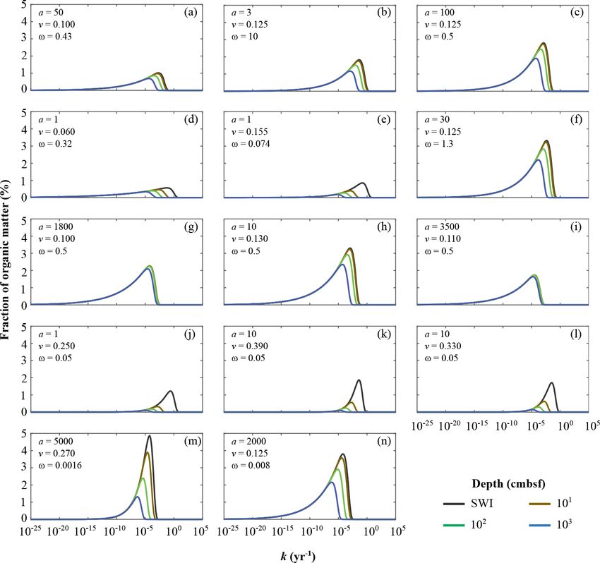
F. S. Freitas et al.: New insights into large-scale trends of apparent organic matter reactivity                                         4653

Table 1. Environmental factors influencing organic matter reactivity in marine sediments.

      Description                                                    Reference
      Sources and composition                                        Burdige (2006), Canfield (1994), Hedges et al. (1997),
                                                                     Meyers (1997), Middelburg (2019)
      Oxygen exposure time (settling and burial)                     Hartnett et al. (1998), Hoefs et al. (2002), Sinninghe Damsté
                                                                     et al. (2002), Huguet et al. (2008), Sun and Wakeham (1994),
                                                                     Wakeham et al. (1997)
      Terminal electron acceptor availability                        Aller (1994), Aller and Aller (1998), Canfield et al. (1993),
                                                                     Canfield (1994)
      Microbial activity                                             LaRowe et al. (2020a, b), Stevenson et al. (2020),
                                                                     Bradley et al. (2020)
      Sediment biological mixing (bioturbation and bioirrigation)    Aller (1980, 1994), Aller and Aller (1998), Boudreau (1994),
                                                                     Grossi et al. (2003), Middelburg (2018),
                                                                     Aller and Cochran (2019)
      Ageing and transport history                                   Bianchi et al. (2018), Cathalot et al. (2010), Griffith et al.
                                                                     (2010), Mollenhauer et al. (2003, 2007), Ohkouchi et al. (2002),
                                                                     Ausín et al. (2021)
      OM–sediment association                                        Bianchi et al. (2018), Hemingway et al. (2019), Keil and Cowie
                                                                     (1999), Mayer (1994b, a)
      OM–iron mineral adsorption                                     Salvadó et al. (2015), Shields et al. (2016), Wang et al. (2019),
                                                                     Faust et al. (2021)
      Priming                                                        van Nugteren et al. (2009), Guenet et al. (2010), Bianchi (2011),
                                                                     Bianchi et al. (2015), Ragavan and Kumar (2021)
      Hydrogen sulfide exposure time (sulfurization)                 Sinninghe Damsté et al. (1988, 1998), Hülse et al. (2019)

LaRowe et al., 2020b; Mayer, 1995; Schmidt et al., 2011;                dation rates and relative contributions of metabolic pathways,
Zonneveld et al., 2010).                                                anaerobic oxidation of methane (AOM) coupled to sulfate re-
   The efforts by Arndt et al. (2013) to develop a general              duction, and fluxes of dissolved species across the sediment–
predictive framework highlighted two critical issues: OM re-            water interface (SWI) at each of the 14 studied sites.
activity is variable within and across settings with no signi-
ficative global trends, and there is a crucial need to resolve
the lack of comparative studies. Therefore, we here use a               2   Study sites
common, integrated model–data approach to inversely deter-
                                                                        Our data–model study covers a wide range of depositional
mine the model parameters that control apparent OM reac-
                                                                        environments, from coastal to shelf and slope settings charac-
tivity from contemporary sediment depth profiles (Sect. 3)
                                                                        terized by widely different environmental conditions (Fig. 1,
at 14 different sites from five different depositional environ-
                                                                        Table 2). It comprises the following benthic provinces
ments (Sect. 2). OM degradation is formulated according to
                                                                        (Seiter et al., 2004): northern European margin (EUR1), NW
the reactive continuum model (RCM) (Boudreau and Rud-
                                                                        Mediterranean margin off Rhone delta (EUR2), western Ara-
dick, 1991), which represents the most suitable degradation
                                                                        bian Sea (WARAB), Bering Sea (NWPAC), and SW At-
model type to explore links between reactivity parameters
                                                                        lantic off La Plata River (RIOPLATA). Most of those re-
and environmental controls (see Sect. 3.2 for details). De-
                                                                        gions are characterized by predominantly temperate climate
rived RCM parameters are discussed in the environmental
                                                                        regimes, except for the Arabian Sea region (arid) and the
context of depositional settings. We further complement the
                                                                        Bering Sea area (snow/polar) (Chen and Chen, 2013). OM
newly derived parameter set with a compilation of previously
                                                                        characteristics also cover a broad spectrum, ranging from
published RCM parameter values to explore the distribution
                                                                        organic-rich (TOC > 2 wt %) to lean (TOC < 1 wt %) sedi-
of model parameters and provide first-order constraints on
                                                                        ments (Premuzic et al., 1982; Seiter et al., 2004) and from
model parametrization in data-poor areas. Finally, we eval-
                                                                        predominantly terrestrial (coast), to mixed terrestrial and ma-
uate the control of OM reactivity on benthic cycling and
                                                                        rine (coast/shelf), to predominantly marine (shelf/slope) OM
fluxes by linking RCM parameters to estimated OM degra-
                                                                        (Hedges et al., 1997; Meyers, 1997). The pelagic ecosys-

https://doi.org/10.5194/bg-18-4651-2021                                                          Biogeosciences, 18, 4651–4679, 2021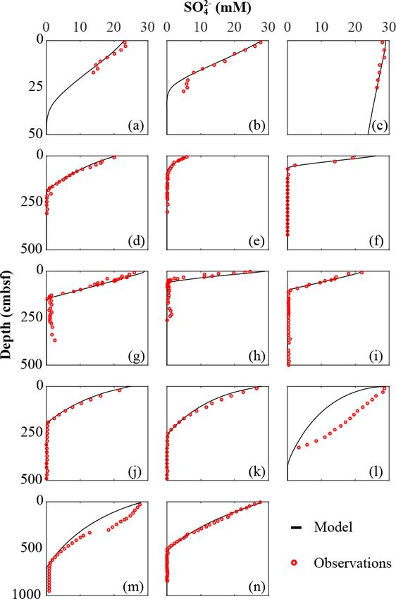
4654 F. S. Freitas et al.: New insights into large-scale trends of apparent organic matter reactivity
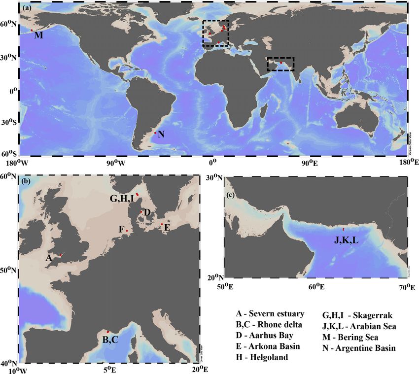
Figure 1. Depositional environment geographic locations. (a) Global scale; (b) European margin; (c) Arabian Sea region. Map produced
with Ocean Data View (Schlitzer, 2019).
tem structure reflects local and regional characteristics. Over- the inverse model approach used to extract RCM parameters
all, as a common characteristic they display the occurrence from the observed depth profiles (Sect. 3.2.4), and a sum-
of spring–summer phytoplankton blooms (e.g. Cowie, 2005; mary of the analysed model output (Sect. 3.2.5).
Rixen et al., 2019; Fleming-Lehtinen and Laamanen, 2012;
Jensen et al., 1990; Coyle et al., 2008). This is also reflected 3.1 Observational data
by the composition of the phytoplankton community and thus
OM production at the photic zone and vertical transport effi- We benefit from previously published datasets to develop
ciency to sediments (e.g. Bach et al., 2019). This wide spec- our large-scale OM reactivity assessments. TOC and pore-
trum of depositional environments (Tables 2 and S1) offers a water SO2−4 depth profiles as well as site-specific physical
unique opportunity to quantify OM reactivity and explore its characteristics and supporting data are available for all sites
multidisciplinary links with environmental drivers. and were compiled from the PANGAEA database (https:
//www.pangaea.de, last access: 20 November 2020) (except
from Rhone delta and Severn estuary datasets), as well as
3 Methods corresponding published literature (see below). Specific de-
tails about sampling strategies and analytical methods can
Here, we adopt an integrated model–data approach to deter- be found in the respective publications. The dataset for the
mine inversely OM reactivity parameters from contemporary Severn estuary (Table 2; row A) is from Thomas (2014).
total organic carbon (TOC) and sulfate (SO2− 4 ) profiles mea- Rhone delta data (Table 2; rows B and C) are from the DI-
sured at 14 sites across the five different depositional envi- CASE project (Rassmann et al., 2016). Data for the north-
ronments described in Sect. 2. The following sections pro- ern European margin sites Aarhus Bay, Arkona Basin, and
vide an overview of the observational data (Sect. 3.1), a brief the Skagerrak transect (Table 2; rows D, E, G, H, and I) are
description of the applied RTM (Sect. 3.2.1; for further de- part of the Europe-funded project METROL (Aquilina et al.,
tails see Supplements, Sect. S2), a detailed description of 2010; Dale et al., 2008a, b; Knab et al., 2008; Mogollón et
Biogeosciences, 18, 4651–4679, 2021 https://doi.org/10.5194/bg-18-4651-2021Table 2. Oceanographic context of depositional environments studied in the large-scale organic matter reactivity quantification.
Site/ Lat (◦ )/ Climate zone/ Setting/ Sed. rate SWI TOC 114 C (‰)/ OM type/
core ID long (◦ ) benthic depth (m) (cm yr−1 )/ redox (wt %)/ Fmod input
province bottom temp. condition OC : SA
(◦ C) (mg m−2 )
A Severn estuary/ 51.50 N/ Temperate/ Coast/ 4.3 × 10⁻¹ / Sub-oxic 3.0/ NA/ Largely terrestrial/
ST-1 3.07 W EUR1 8 18.0 NA NA fluvial
B Rhone proximal zone/ 43.31 N/ Temperate–Mediterranean/ Coast/ 1.0 × 101 / Oxic 2.0/ 143 ± 14/ Largely terrestrial and aquatic/
A 4.85 E EUR2 19 15.0 NA NA fluvial
C Rhone shelf/ 43.27 N/ Temperate–Mediterranean/ Shelf/ 5.0 × 10⁻¹ / Oxic 1.3/ −218 ± 9/ Mixed terrestrial and marine/
https://doi.org/10.5194/bg-18-4651-2021
C 4.77 E EUR2 74 14.0 0.4–0.7 NA fluvial and pelagic
D Aarhus Bay/ 56.11 N, Temperate, Coast, 3.2 × 10⁻¹ , Sub- 3.5/ NA/ Largely terrestrial with marine contribution/
173GC, 174GC 10.34 E EUR1 15 9.0 oxic/anoxic NA NA fluvial and pelagic
(summer)
E Arkona Basin/ 54.80 N/ Temperate/ Shelf/ 7.4 × 10⁻³ / Sub-oxic 5.0/ NA/ Mostly terrestrial/
348GC, 351GC 13.78 E EUR1 43 5.0 NA NA fluvial
F Helgoland mud area, North Sea/ 54.08 N/ Temperate/ Shelf/ 1.3 × 100 / Anoxic 1.1/ −174–195/ Largely terrestrial with marine contribution/
HE443-010 7.97 E EUR1 29 10.0 NA NA pelagic and fluvial
G Skagerrak S10/ 57.92 N/ Temperate/ Shelf/ 5.0 × 10⁻¹ / Oxic 1.3/ NA/ Largely terrestrial/
807GC, 808GC 9.75 E EUR1 86 8.7 0.6–0.7 NA fluvial and pelagic
H Skagerrak S11/ 57.95 N/ Temperate/ Shelf/ 5.0 × 10⁻¹ / Oxic 0.5/ NA/ Largely terrestrial/
816GC, 836GC 9.70 E EUR1 150 9.8 0.6–0.7 NA fluvial and pelagic
I Skagerrak S13/ 58.05 N/ Temperate/ Slope/ 5.0 × 10⁻¹ / Oxic 1.8/ NA/ Largely terrestrial/
786GC, 789GC 9.60 E EUR1 386 4.5 0.6–0.7 NA fluvial and pelagic
J Arabian Sea (core of OMZ)/ 24.88 N/ Arid/ Slope/ 5.0 × 10⁻² / Anoxic 0.92/ NA/ Largely marine/
GeoB 12312 63.02 E WARAB 654 11.6 1.1–2.3 0.800–0.920 pelagic
K Arabian Sea (OMZ transition)/ 24.81 N/ Arid/ Slope/ 5.0 × 10⁻² / Anoxic 0.89/ NA/ Largely marine/
GeoB 12309 62.99 E WARAB 957 9.6 1.1–2.3 0.800–0.920 pelagic
L Arabian Sea (below OMZ)/ 24.71 N/ Arid/ Slope/ 5.0 × 10⁻² / Oxic 0.87/ NA/ Largely marine/
GeoB 12308 62.99 E WARAB 1586 5.1 0.4–1.1 0.800–0.920 pelagic
F. S. Freitas et al.: New insights into large-scale trends of apparent organic matter reactivity
M Bering Sea/ 54.57 N/ Snow/polar/ Slope/ 1.6 × 10⁻³ / Oxic 1.3/ −143/ Largely marine/
SO202-22 168.81 W NWPAC 1476 2.0 NA 0.857 pelagic
N Argentine Basin/ 39.31 S/ Temperate/ Slope/ 8.0 × 10⁻³ / Oxic 1.0/ NA/ Mixed marine and terrestrial/
GeoB 13863 53.95 W RIOPLAT 3687 3.5 NA 0.777 pelagic and lateral transport
NA: not available.
Biogeosciences, 18, 4651–4679, 2021
46554656 F. S. Freitas et al.: New insights into large-scale trends of apparent organic matter reactivity
al., 2012). Data from the Helgoland mud area, North Sea to 1500 cm, due to the low sedimentation rate assumed for
(Table 2; row F) (Henkel and Kulkarni, 2015), the Arabian this site (Table 2). This choice is based on initial tests and en-
Sea oxygen minimum zone (OMZ) transect (Table 2; rows J, sures that the model domain covers the diagenetically most
K, and L) (Bohrmann and cruise participants, 2010a, b, c), active zone, thus reducing the influence of biogeochemical
Bering Sea (Table 2; row M) (Gersonde, 2009), and Argen- dynamics in underlying sediments on biogeochemical dy-
tine Basin (Table 2; row N) (Henkel et al., 2011) are pre- namics within the model domain. The model equations were
sented in the PANGAEA database (see above). We use those solved on an uneven grid and with a time-adapting time step
site-specific datasets to inform our data–model analysis and (1t < 0.01) run until steady state was reached. The Sup-
to constrain OM reactivity and related benthic processes. plement includes a detailed description of the general RTM
framework used here, its parametrization, and its numerical
3.2 Model description solution (Sect. S2).
3.2.1 General RTM framework 3.2.2 OM degradation model
The Biogeochemical Reaction Network Simulator (BRNS) OM is composed of a complex and dynamic mixture of com-
(Aguilera et al., 2005; Regnier et al., 2002) is an adaptive pounds that are distributed over a wide, continuous spec-
simulation environment that has been successfully employed trum of reactivities. Thus, OM degradation is described by
to reproduce and quantify diagenetic processes in marine the reactive continuum model (RCM) (Boudreau and Rud-
sediments across a wide range of depositional environments dick, 1991), which assumes a continuous distribution of OM
and timescales (Dale et al., 2008a; Thullner et al., 2009; compounds over the entire reactivity spectrum. The RCM
Wehrmann et al., 2013). The BRNS is suitable for large, assumes a gamma distribution to describe the probability
mixed kinetic–equilibrium reaction networks (Dale et al., density function of OM distribution, om(k, t) (Aris, 1968;
2009; Jourabchi, 2005; Thullner et al., 2009). The concen- Boudreau and Ruddick, 1991; Ho and Aris, 1987). The over-
tration depth profiles of solid and dissolved species in marine all rate of OM degradation RTOC is given by the integral
sediments are calculated according to the vertically resolved Z ∞
mass conservation equation of solid and dissolved species in rn = RTOC = − k · om (k, t) dk. (2)
porous media (Berner, 1980; Boudreau, 1997): 0
∂σ Ci ∂
∂Ci ∂Ci
∂σ ωCi Here, om(k, t) determines the concentration of OM having a
= Dbio σ + Di σ − degradability between k and k + dk at time t, with k being
∂t ∂z ∂z ∂z ∂z
X equivalent to the first-order degradation rate constant. The
+ αi σ (Ci (0) − Ci ) + snr .
n i n
(1) initial distribution (t = 0) of OM is given by
The first three terms on the right-hand side represent the TOC(0) · a v · k v−1 · e−a·k
transport process (bioturbation and molecular diffusion, ad- om(k, 0) = , (3)
0(v)
vection, and bioirrigation), whereas the last term denotes the
sum of all reactions (production and consumption) affecting where TOC(0) denotes the initial OM content, 0(v) is the
species i. Table 2 summarizes all symbols employed here. gamma distribution, a is the average lifetime of the more
Briefly, the implemented reaction network encompasses reactive components of bulk OM, and v represents the di-
the most pertinent primary and secondary redox reactions mensionless scaling parameter of the distribution near k = 0.
found in the upper layers of marine sediments (e.g. Aguilera The free, positive parameters a and v delineate the shape of
et al., 2005; Thullner et al., 2009; Van Cappellen and Wang, the initial distribution of OM compounds along the range of
1996; Wang and Van Cappellen, 1996). It explicitly accounts k, and thus the overall reactivity of bulk OM. As such, the
for the heterotrophic degradation of OM coupled to the con- RCM approach requires the definition of two parameters that
sumption of oxygen (aerobic OM degradation), nitrate (den- will define the shape of the OM distribution over reactivity k
itrification), sulfate (organoclastic sulfate reduction), and (Sect. 3.2.5, Eq. 5).
methanogenesis. Additionally, the reaction network accounts Due to the rapid depletion of the most reactive compounds,
for secondary redox reactions, i.e. re-oxidation of reduced the reactivity of the bulk material decreases during degrada-
species produced during primary redox reactions. It explic- tion, reflecting the widely observed reactivity decrease with
itly resolves nitrification, sulfide re-oxidation by O2 , anaer- burial time, depth, and age (Boudreau and Ruddick, 1991;
obic oxidation of methane (AOM) coupled to sulfate reduc- Middelburg, 1989). This indicates that degradation of OM
tion, and CH4 reoxidation by O2 . proceeds at different rates in parallel. Interactions between
The model transport and reaction equations were solved different compounds or transformations of compounds can
sequentially according to Regnier et al. (1998). The size of change the reactivity of a given compound. While the RCM
the model domain was fixed at 1000 cm for all sites, except does not explicitly account for such interactions and trans-
for the Bering Sea, in which the model domain was extended formations, the overall OM profiles take these interactions
Biogeosciences, 18, 4651–4679, 2021 https://doi.org/10.5194/bg-18-4651-2021F. S. Freitas et al.: New insights into large-scale trends of apparent organic matter reactivity 4657
implicitly into account. Thus, OM compounds are continu- 3.2.4 Inverse modelling
ously and dynamically distributed over a range of reactivities
that capture the decrease in apparent reactivity with burial We use an inverse model approach to extract the optimal OM
age and depth as the most reactive compounds are succes- reactivity parameter set a and v (i.e. the apparent OM reac-
sively degraded. The interplay of a and v drives the bulk OM tivity) by assuming that the rank of a parameter set depends
reactivity depth profiles and consequently the yielded pro- on the similarity between simulated and measured data. In
files from the reaction network implemented in the BRNS. general, all inverse modelling approaches are ultimately af-
The evolution of OM concentration as a function of depth z fected by a few limitations. Among others, the quality of the
is given by inverse modelling results is directly affected by the quality
v of the observational data. In particular, the lack of observa-
a tions and data at the SWI due to core top loss during sed-
TOC (z) = TOC(0) · , (4)
a + age(z) iment sampling by gravity and piston corers can impact re-
sults. Additionally, processes that are not explicitly described
where a and v are the free RCM parameters (Arndt et al., in the applied model can impact inverse model results be-
2013; Boudreau and Ruddick, 1991) and age(z) denotes the cause reaction rate parameters implicitly account for those
age of the sediment layer at depth z. For non-bioturbated processes. Furthermore, downcore changes in concentration–
sediments (z > zbio ) the burial age(z) can be calculated as depth profiles may also be influenced by transient features
a function of the burial velocity (Sect. S2.3, Eq. S8). How- in bottom water conditions and/or fluxes, and the validity of
ever, within the bioturbated upper sediment layers, the age the steady-state assumption thus needs to be carefully eval-
distribution of reactive species is controlled by both sedimen- uated. Finally, multiple parameter sets might fit the observa-
tation, bioturbation, and the reactivity k of reactive species tions equally well. Because both a and v exert an influence
(Meile and Van Cappellen, 2005). In such cases, we apply a on the apparent OM reactivity and its evolution with depth
multi-G approximation for the RCM in the bioturbated sedi- (see below, Eq. 5), they are not completely independent pa-
ments (Sect. S2.3, Eqs. S9–S18). rameters. For instance, a decrease in v (decreasing reactivity)
can be compensated for by a simultaneous decrease in pa-
3.2.3 Boundary conditions
rameter a (increasing reactivity). Consequently, different a
Boundary conditions place the BRNS in the environmental and v parameter couples might result in equally statistically
context of each of the study sites (Table 4). The boundary satisfying fits between the simulated and observed profiles.
conditions are constrained based on either site-specific mea- These limitations can be alleviated by using comprehen-
surements or alternatively published data if direct observa- sive, multi-component observational datasets, because the in-
tions were not available. Here, we assume a fixed bound- clusion of additional information adds further constraints.
ary concentration of OM at the SWI. Concentrations of O2 However, such datasets are often not available. For instance,
are based on measurements in Skagerrak (Canfield et al., the first efforts to quantify a and v parameter values, and
1993) and the Rhone delta (Rassmann et al., 2016) sedi- thus reactivity, on the basis of observations solely focused
ments. Similarly, concentrations of NO− on downcore TOC profiles (Boudreau and Ruddick, 1991).
3 are based on mea-
surements in Skagerrak sediments (Canfield et al., 1993). Such an approach was instrumental for the development of
Because of the lack of site-specific information, these O2 the RCM and for producing the first large-scale dataset of
and NO− a and v. However, the increasing availability and accessi-
3 measurements are adopted at all oxic sites (where
2− bility of multi-species datasets allow for the use of addi-
SO4 >28 mM) since they are representative for coastal and
tional information that is available across different sites. Be-
shallow slope sites, and their exact value exerts no influ-
cause OM heterotrophic degradation is the driver behind bio-
ence on deep SO2− 4 and CH4 concentrations. For anoxic geochemical dynamics in marine sediments, downcore pro-
sites (where SO2− −
4 < 28 mM), O2 and NO3 bottom water
2−
files of TEAs (e.g. SO2− 4 ) (e.g. Bowles et al., 2014; Jør-
concentrations are set to zero. SO4 concentrations were gensen et al., 2019b) or reduced products of OM degradation
constrained based on measurements for each simulated site. (such as CH4 and NH+ 4 ) could be used as further constraints.
Concentrations of CH4 and HS− were set to zero at SWI, However, data availability is often still limited; therefore,
as those species are rapidlyoxidized in the overlying bottom it is important to identify a minimum set of observational
water. A no-flux ∂C ∂z = 0 condition was implemented for data that are widely available and comparably easy to mea-
all species at the lower boundary, assuming that biogeochem- sure. We tested the suitability of different artificial porewa-
ical dynamics in underlying sediments exert no influence on ter datasets for the inverse determination of apparent OM re-
diagenetic processes in the model domain (e.g. Thullner et activity. Using an artificially generated dataset (see Supple-
al., 2009). ment Sect. S3), we ran the BRNS in the same fashion as we
did for the site-specific data–model approach (see below).
Our sensitivity analysis confirms that when TOC is consid-
ered as a single constraint, multiple pairs of a and v pro-
https://doi.org/10.5194/bg-18-4651-2021 Biogeosciences, 18, 4651–4679, 20214658 F. S. Freitas et al.: New insights into large-scale trends of apparent organic matter reactivity
duce equivalent TOC depth profiles (Supplement Fig. S1). sible a–v space (see above) was sampled on a coarse regular
Model results show that including SO2− 4 depth profiles as grid (1 log(a) = 1, 1v = 0.02), and, for each of these runs, r,
an additional constraint (Supplement Fig. S2) facilitates the RMSD, and SD were calculated for both TOC and SO2− 4 pro-
identification of a best-fit a and v parameter set (Supplement files. Based on these measures, a new, more finely resolved
Fig. S3). CH4 profiles were used as an additional qualita- a–v grid (10 × 10) was defined around the a–v couples that
tive constraint when the data were available, although mea- showed the smallest combined misfit between simulated and
sured ex situ CH4 profiles are often not reliable due to sam- observed TOC and SO2− 4 profiles. On this grid, a–v couples
pling and measurement uncertainties in deeper sediment lay- were again sampled regularly, and the optimized a–v couple
ers where concentrations exceed millimolar levels (Dale et was determined by the lowest combined misfit (Table 5).
al., 2008a; Hensen et al., 2003; Hilligsøe et al., 2018). The
dynamics of SO2− 3.2.5 Quantification of organic matter reactivity and
4 and CH4 are solely controlled by OM
degradation and AOM (e.g. Bowles et al., 2014; Egger et associated benthic processes
al., 2018; Regnier et al., 2011), although their distributions
can also be affected by bioirrigation in particularly shallow The apparent reactivity of bulk OM k for each site is cal-
sulfate–methane transition zones (SMTZs) (e.g. Dale et al., culated based on the RCM reactivity parameters a and v
2019). In anoxic settings and deeply buried sediments, SO2− (Boudreau and Ruddick, 1991) that yield the best data–model
4
is the dominant TEA and CH4 is the most common reduced fit and is given by
species (Jørgensen et al., 2019a, b). Thus, a combination of v
k(z) = . (5)
TOC, SO2− 4 , and CH4 (if available to verify the depths of
(a + age(z))
the SMTZ) depth profiles incorporates the information con- The apparent reactivity of bulk OM at the sediment–water
tained in the observed benthic sulfur and carbon dynamics interface (z = 0) is thus given by
and is sufficient to extract robust estimates of apparent OM v
reactivity and its evolution from the sediment–water inter- k(0) = . (6)
a
face down to the SMTZ. In addition, because changes in a–v
exert different effects on TOC and SO2− The BRNS simulates downcore concentration profiles for
4 depth profiles (see
Figs. S1 and S2), including these two species reduces the each species i that is explicitly resolved in the reaction net-
impact of the a–v correlation on the uniqueness of fit. Thus, work, as well as reaction rates rn (Table S4). From those re-
here we perform a site-specific data–model fit based on TOC action rates, the total rate of organic carbon oxidation, i.e.
and SO2− the depth integral of OM degradation for each primary redox
4 (and CH4 ) depth profiles.
The optimal parameter set was then determined for each reaction n, can be calculated by integrating the rate over the
site by assuming that the rank of a parameter set depends on entire model domain L (e.g. Thullner et al., 2009):
Z L Z ∞
the similarity between simulated and measured data. Best-fit X
parameter couples were found by minimizing the misfit be- RTOC, total = n=1−4
rn dx = − k · om (k, t) dk, (7)
0 0
tween model results and simulations. We quantified the sim-
ilarity between the simulated and observed TOC and SO2− where n = 1, 2, 3, and 4 denote aerobic OM degradation,
4
depth profiles in terms of correlation coefficient (r), centred denitrification, organoclastic sulfate reduction, and methano-
root-mean-square difference (RMSD), and standard devia- genesis, respectively (Table S4). The OM fluxes (Jin ) at the
tions (SD). All these measures can be graphically represented SWI are calculated as the sum of OM out of the sediment
in a single Taylor diagram (Taylor, 2001) that statistically (JOM,out ) and the burial fluxes at the base of the model do-
quantifies the misfit between the observed and simulated data main (JOM,bur ) (e.g. Burdige, 2006). Here, we assume that
and visualizes how closely the simulated depth profile resem- JOM,out is equivalent to the depth-integrated rates of OM
bles the observed one. degradation (Eq. 7) and JOM,bur is solely governed by ad-
The best-fit RCM parameters were inversely determined vective processes at depth z = 1000 cm. As such
Z L
by first running the model for each site with a set of a– X
v couples over the entire range of previously published a JOM,out = n=1−4
rn dx, (8)
0
(a = 10−3 –107 year) and v (v = 10−2 –100 ) values (Arndt et
JOM,bur = (1 − ϕz ) · ωz · TOCz , (9)
al., 2013, and references therein). The approach adopted for
the sampling of the parameter space is a critical step in in- JOM,in = JOM,out + JOM,bur . (10)
verse modelling since the chosen statistical measures may Additionally, the fluxes of species i at the SWI, i.e. the
reveal, in addition to a global optimum, multiple local op- benthic–pelagic fluxes, are calculated from the model-
tima. Because of the comparably low computational cost of derived depth profiles of species i according to e.g. Bur-
the forward modelling, the low number of unknown param- dige (2006):
eters (here, a and v), and the weak nonlinearity of the prob-
lem, we used a simple two-step nested regular sampling of Ji = Ji,Advection + Ji,Diffusion
the two-dimensional parameter space. First, the entire plau- + Ji,Bioturbation + Ji,Bioirrigation . (11)
Biogeosciences, 18, 4651–4679, 2021 https://doi.org/10.5194/bg-18-4651-2021F. S. Freitas et al.: New insights into large-scale trends of apparent organic matter reactivity 4659
4.1 Constraining apparent OM reactivity
4.1.1 Inverse modelling
We inversely determined the set of RCM parameters a and v
that produces the best model fit to the observed TOC (Fig. 2)
and SO2−4 (Fig. 3) depth profiles. Table 5 shows the quantita-
tive assessments of these model fits and associated uncertain-
ties. Overall, TOC profiles display a satisfying fit between
model and observations. However, the quality of fit is often
compromised by a lack of observations and data at the SWI
due to core loss during sediment sampling by gravity and
piston corers, poor downcore sampling resolution, and pos-
sible non-steady-state conditions. Generally, the latter may
be problematic when trying to reproduce sedimentary con-
ditions of dynamic shallow systems and long-term burial in
shelf and deep-sea sites. At estuarine sites, steady-state con-
ditions may be impacted by the highly dynamic nature of
such settings. The Severn estuary exhibits strong tidal dy-
namics that result in continuous cycles of sediment resus-
pension (Manning et al., 2010). The Rhone delta experiences
strong pulses of fresh water and sediments associated with
flood events, as well as variable sedimentation rates (An-
tonelli et al., 2008; Cathalot et al., 2010; Zebracki et al.,
2015). In shelf and slope settings, steady-state assumptions
can be impacted by fluctuations on sedimentation rates and
lateral transport of sediments across shelves (e.g. Henkel et
al., 2011; Riedinger et al., 2014, 2017; Hensen et al., 2003;
Cowie, 2005). Further, due to the possible loss of the upper
few millimetres to centimetres during sampling with grav-
Figure 2. Total organic carbon data–model best fit: (a) Severn ity and piston cores, it can be challenging to quantify OM
estuary; (b) Rhone pro-delta; (c) Rhone shelf; (d) Aarhus Bay; contents at the SWI. Some of our sites (e.g. northern Eu-
(e) Arkona Basin; (f) Helgoland mud area, North Sea; (g) Skagerrak ropean sites; Aquilina et al., 2010; Knab et al., 2008) are
– S10; (h) Skagerrak – S11; (i) Skagerrak – S13; (j) Arabian Sea – likely to be impacted by such factors. Overall, such limita-
OMZ core; (k) Arabian Sea – OMZ transition; (l) Arabian Sea –
tions in inverse model results are highlighted by the some-
below OMZ; (m) Bering Sea; (n) Argentine Basin.
what low correlation coefficients for TOC profiles in most
cases (rTOC < 0.75; Table 3). We find that adding additional
Positive Ji values indicate upward fluxes from the sediment, constraints to the model–data fit relieves such limitation.
whereas negative values represent downward fluxes into the The SO2− 4 depth profiles (Fig. 3) display a good agreement
sediment. between present-day observations and model simulations,
with the majority of sites exhibiting high correlation coef-
ficients (rSO4 >0.95; Table 3). Nevertheless, Fig. 3 shows
4 Results and discussion cases where the model-derived sulfate depth profiles display
some mismatches relative to observations (Arabian Sea be-
The integrated data–model analysis yielded a comprehen- low OMZ, Fig. 3l; Bering Sea, Fig. 3m). At the Bering Sea,
sive picture of OM reactivity parameters (a, v, and k(z)), the data–model discrepancy is likely associated with kinks in
as well as OM degradation dynamics and benthic–pelagic both TOC (Fig. 2m) and SO2− 4 (Fig. 3m) profiles. They likely
coupling for our large-scale compilation of depositional en- represent changes in the depositional regime over the studied
vironments (Table 6). Because model parameters implicitly timescale (e.g. Hensen et al., 2003) that are not captured by
account for all the processes that are not explicitly described the model. The mismatch in the Arabian Sea at the site be-
in the model, this variability provides important insights into low the OMZ (Fig. 3l) could originate from SO2− 4 recycling
the environmental controls on OM reactivity. through H2 S oxidation by MnO2 and Fe(OH)3 (e.g. Rass-
mann et al., 2020; Schulz et al., 1994); however we are un-
able to further explore this hypothesis due to a lack of metal
oxide data to constrain those biogeochemical reactions.
https://doi.org/10.5194/bg-18-4651-2021 Biogeosciences, 18, 4651–4679, 20214660 F. S. Freitas et al.: New insights into large-scale trends of apparent organic matter reactivity
Table 3. Summary of model elements incorporated in the BRNS.
Symbol Description
Chemical species, i
TOC Total organic carbon
CH2 O Organic matter (simplified stoichiometry)
O2 Oxygen
NO−3 Nitrate
SO2−
4 Sulfate
CH4 Methane
NH+4 Ammonium
PO3−
4 Phosphate
HS− Sulfides
Model parameters
Ci Concentration of species i
t Time
z Sediment depth
L Length of model domain
T Temperature
S Salinity
h Water depth
σ Porosity term solid species, σ = 1 − ϕ dissolved species, σ = ϕ
ϕ Sediment porosity
Di Effective molecular diffusion coefficient of dissolved species i
Dbio Bioturbation diffusion coefficient
zbio Depth of bioturbated zone – sediment mixed layer
ω Burial velocity – sedimentation rates
αi Bioirrigation coefficient
sin Stoichiometric coefficient of species i
n Kinetically controlled reaction
rn Reaction rate
ki First-order reaction rate constant
0(v) Gamma distribution
a Reactive continuum model shaping parameter
v Reactive continuum model scaling parameter
om(k, t) Probability density function of OM distribution
Quantification of model-derived parameters
k(z) Apparent organic matter reactivity at a given depth
RTOC Organic matter degradation rate
RTOC, total Depth integrated organic matter degradation rates
JOM,in Fluxes of organic matter at the sediment–water interface
JOM,out Fluxes of organic matter consumed by heterotrophic degradation
JOM,bur Fluxes of organic matter buried (below model domain, L)
Ji Fluxes of species i at the sediment–water interface
4.1.2 Apparent OM reactivity parameters v and a et al., 2012; Mewes et al., 2016; Mogollón et al., 2012, 2016;
Wehrmann et al., 2013; Ye et al., 2016), they provide useful
constraints on the plausible range of a and v, as well as their
The inversely determined OM reactivity parameters a and v control on the global variability in apparent OM reactivity.
(Sect. 3.2.4) derived from the best-fit model solutions (Ta- Parameter v exerts a scaling influence on OM reactivity
ble 6) reveal important differences in apparent OM reactiv- distribution. High v values result in a high initial OM re-
ity and its distribution on a global scale. Alongside a and v activity, whereas low v values produce low initial reactivity
parameters compiled from the literature (Arndt et al., 2009; (Arndt et al., 2013). For instance, an extremely low v value of
Boudreau and Ruddick, 1991; Contreras et al., 2013; Henkel
Biogeosciences, 18, 4651–4679, 2021 https://doi.org/10.5194/bg-18-4651-2021F. S. Freitas et al.: New insights into large-scale trends of apparent organic matter reactivity 4661
burg, 1989), which applies a globally constant parameter of
0.16:
k (z) = 0.16 · (a + age(z))−0.95 . (12)
Although the parameters of the so-called power model can-
not be directly compared to those of the RCM due to different
exponents, the RCM is nevertheless equivalent to a general
power law with an exponent of −1:
k (z) = v · (a + age(z))−1 . (13)
Thus, the v parameter range of the RCM is in good agree-
ment with the 0.16 value imposed in the power-law model.
Nevertheless, our results also reveal exceptions. Particu-
larly high v values (v > 0.25) were determined for the Ara-
bian Sea and Bering Sea. Similarly, Boudreau and Rud-
dick (1991) also report exceptionally high values (v ≈ 1) for
the Peru Margin and north Philippine Sea but invoked the
possibility of non-steady-state depositional conditions as a
possible explanation. In our study, v>0.25 also coincides in
part with the poorest data–model fits, such that the robust-
ness of such high v values is uncertain (Table 5). In particu-
lar, the high v value in the Bering Sea (Table 6) might result
from uncertainties (see above, Sect. 4.1.1) associated with
boundary conditions and transient features (e.g. Henkel et
al., 2011; Hensen et al., 2003). However, the model-derived
v > 0.25 for the Arabian Sea agrees with previous diagenetic
model results for that region. Luff et al. (2000) developed a
3G model to investigate OM dynamics and found that bulk
OM contains exceptionally reactive compounds with first-
Figure 3. Sulfate data–model best fit: (a) Severn estuary; (b) Rhone order k of 0.2–30 yr−1 . In the Arabian Sea, the OM flux to the
pro-delta; (c) Rhone shelf; (d) Aarhus Bay; (e) Arkona Basin;
sediment is supported by high primary production rates dur-
(f) Helgoland mud area, North Sea; (g) Skagerrak – S10; (h) Sk-
ing the monsoon season (e.g. Cowie, 2005), complemented
agerrak – S11; (i) Skagerrak – S13; (j) Arabian Sea – OMZ core;
(k) Arabian Sea – OMZ transition; (l) Arabian Sea – below OMZ; by deep carbon fixation by microorganisms (Lengger et al.,
(m) Bering Sea; (n) Argentine Basin. 2019). Observations indicate an efficient vertical transport of
diatom and haptophyte detritus to the sediment (Barlow et al.,
1999; Cowie, 2005; Latasa and Bidigare, 1998; Shalapyonok
et al., 2001). High transport rates and pronounced oxygen
≤ 0.01 for OM deposited during the late Cretaceous Oceanic minimum zones might limit heterotrophic degradation of the
Anoxic Event 2 at Demerara Rise (Arndt et al., 2009) has sinking OM in the water column, thus delivering comparably
been linked to intense and rapid sulfurization of OM in the unaltered OM to the sediment. Biomarker analysis of benthic
strongly euxinic subtropical Atlantic Ocean (Hülse et al., OM indicates the deposition of highly reactive OM (Koho et
2019). While previously published values for contemporary al., 2013) and a reactivity decrease with extended exposure
ocean sediments fall within the range of 0.1 to 1.08 (Arndt to oxic conditions in the water column (Vandewiele et al.,
et al., 2013; Boudreau and Ruddick, 1991), inversely deter- 2009). Therefore, the somewhat atypical high v values deter-
mined v values predominantly fall within the range of 0.1– mined (together with comparably low a values; see below)
0.2 (apparent 6th–11th order of reaction) – although lower for the Arabian Sea OMZ transect are supported by interdis-
and higher v values were also determined (Fig. 4a). Newly ciplinary observations. Thus, v has a relatively narrow range
determined v parameters thus confirm the previously ob- of 0.1 to 0.2, with higher > 0.2 values generally restricted
served dominance of v values between 0.1 and 0.2 (Boudreau to depositional environments that are characterized by high
and Ruddick, 1991) and suggest that v is relatively constant primary production rates, anoxic water conditions, and en-
across a wide range of different depositional environments hanced vertical OM fluxes within the OMZ.
encountered in the contemporary ocean. These findings also Parameter a determines both the overall apparent reactiv-
agree with the parametrization of another empirically derived ity and the shape of the reactivity decrease with depth. High
continuum model description of OM degradation (Middel- a values result in an overall low OM reactivity, but a slow
https://doi.org/10.5194/bg-18-4651-2021 Biogeosciences, 18, 4651–4679, 20214662 F. S. Freitas et al.: New insights into large-scale trends of apparent organic matter reactivity
Figure 4. Frequency histogram of organic matter reactivity parameter distribution on a global scale: (a) scaling parameter – v; (b) shaping
parameter – a.
Table 4. Site-specific transport parameters and upper boundary conditions implemented in the reaction–transport model.
Site-specific transport parameters Site-specific upper boundary conditions
Site ϕ Dbio zbio ω T S h TOC O2 NO−
3 SO2−
4 CH4 HS−
cm2 yr−1 cm cm yr−1 ◦C m wt % µM µM mM µM mM
A 0.70 29.8 9 4.3 × 10⁻¹ 18.0 35 8 3.0 0 30 23 0 0
B 0.80 0.50 10 1.0 × 101 16.8 35 18 2.0 245 25 28 0 0
C 0.83 10.0 10 5.0 × 10⁻¹ 14.4 35 75 1.3 225 25 29 0 0
D 0.86 0 0 3.2 × 10⁻¹ 12.0 35 15 3.5 0 0 20 0 0
E 0.86 0 0 7.4 × 10⁻³ 5.0 35 43 5.0 0 0 6 0 0
F 0.70 0 0 1.3 × 100 10.0 35 30 1.1 0 0 26 0 0
G 0.44 27.8 10 5.0 × 10⁻¹ 8.7 35 86 1.3 250 25 29 0 0
H 0.47 26.3 10 5.0 × 10⁻¹ 9.8 35 147 0.5 250 25 29 0 0
I 0.50 0 0 5.0 × 10⁻¹ 4.5 35 386 1.8 0 0 22 0 0
J 0.60 0 0 5.0 × 10⁻² 11.6 35 632 5.0 0 0 25 0 0
K 0.60 0 0 5.0 × 10⁻² 9.6 35 930 4.4 0 0 28 0 0
L 0.70 7.3 10 5.0 × 10⁻² 5.1 35 1,552 4.3 250 25 29 0 0
M 0.60 7.8 10 1.6 × 10⁻³ 2.0 35 1,469 1.3 250 25 28 0 0
N 0.70 1.0 10 8.0 × 10⁻³ 3.5 35 3,687 1.0 250 25 28 0 0
decrease in reactivity with depth. In contrast, low a values gest that the variability of parameter a exerts the major con-
result in a higher reactivity but also a more rapid decrease in trol on the spatial variability in OM reactivity. Additionally,
reactivity with sediment depth (Arndt et al., 2013). Parameter inversely determined a values also broadly agree with previ-
a is often related to the degree of “pre-ageing” or degrada- ously observed global patterns. Low values (a < 102 years;
tion (e.g. Middelburg, 1989; Middelburg et al., 1993). Very i.e. high apparent OM reactivity) are generally determined
fresh marine OM has been shown to be characterized by sub- for depositional environments that are characterized by the
stantially low a values (a = 3.1×10⁻⁴ years) (Boudreau and rapid deposition of predominantly fresh marine OM (e.g.
Ruddick, 1991), while the heavily sulfurized OM deposited Arabian Sea and shallow sites at the northern European mar-
during Cretaceous Oceanic Anoxic Event 2 in the strongly gin), while depositional settings that receive pre-degraded
euxinic subtropical Atlantic Ocean is characterized by very OM and/or complex mixtures of OM (e.g. Skagerrak) exhibit
high a values (a = 104 years) (Arndt et al., 2009). Our in- high a (a > 103 years). However, despite the broad range
versely derived a values span several orders of magnitude of a values, the ensemble of inversely determined a values
(Table 6; Fig. 4b). They thus corroborate the high variability shows that most values fall into the range of 100 −104 years,
observed in previously published a-value compilations (e.g. thus narrowing the range of a values.
Arndt et al., 2013; Boudreau and Ruddick, 1991) and sug-
Biogeosciences, 18, 4651–4679, 2021 https://doi.org/10.5194/bg-18-4651-2021F. S. Freitas et al.: New insights into large-scale trends of apparent organic matter reactivity 4663
Table 5. Summary of statistical tests for the best-fit a–v pair at each site derived from Taylor diagrams.
Reactivity TOC SO2−
4
parameters
Site a v Mean SD RMSD r Mean SD RMSD r
A 5.0 × 101 0.100 data 2.97 0.03 18.49 3.57
model 4.90 1.62 1.64 0.513 17.51 3.44 0.82 0.947
B 3.0 × 100 0.125 data 1.96 0.02 14.10 8.07
model 1.92 0.16 0.14 0.640 12.59 9.18 1.79 0.974
C 1.0 × 10² 0.125 data 1.28 0.01 27.51 0.80
model 1.29 0.01 0.005 0.9998 27.76 0.89 0.37 0.823
D 1.0 × 100 0.060 data 2.41 0.11 6.00 6.18
model 1.63 0.86 0.77 0.738 5.51 5.83 0.57 0.994
E 1.0 × 100 0.155 data 2.17 0.60 1.54 1.83
model 1.79 0.46 0.40 0.561 1.35 1.84 0.23 0.984
F 3.0 × 101 0.125 data 0.89 0.22 1.71 4.93
model 0.89 0.08 0.25 0.014 1.75 5.18 0.76 0.980
G 1.8 × 10³ 0.100 data 1.12 0.45 9.54 9.15
model 1.34 0.00 0.45 0.597 9.70 10.08 1.52 0.984
H 1.0 × 101 0.130 data 0.47 0.18 4.40 7.10
model 0.38 0.04 0.20 0.240 5.88 8.84 2.73 0.931
I 3.5 × 10³ 0.110 data 1.69 0.34 3.51 5.84
model 1.84 0.00 0.34 0.002 3.35 6.23 0.64 0.993
J 1.0 × 100 0.250 data 0.67 0.13 3.26 5.67
model 0.78 0.22 0.19 0.289 2.81 5.21 0.50 0.999
K 1.0 × 101 0.390 data 0.56 0.12 5.30 7.79
model 0.48 0.24 0.22 0.154 4.73 6.97 0.90 0.998
L 1.0 × 101 0.330 data 0.49 0.15 17.67 7.45
model 0.78 0.42 0.33 0.544 9.62 6.14 2.74 0.878
M 5.0 × 10³ 0.270 data 0.82 0.34 10.38 9.93
model 0.94 0.17 0.24 0.566 7.52 7.74 2.79 0.961
N 2.0 × 10³ 0.125 data 0.84 0.07 7.56 8.89
model 0.78 0.12 0.10 0.298 7.32 8.72 0.62 0.995
4.1.3 OM reactivity distributions the changes in OM−reactivity distributions at the consid-
ered burial depths are not entirely driven by differences in
reactivity, but more broadly reflect different exposure to het-
Inversely determined parameters a and v also allow the as- erotrophic degradation across sites.
sessment of the apparent OM reactivity evolution during The Arabian Sea region (Fig. 5j–l) is characterized by the
burial. Here, we calculate the probability distribution of OM deposition of highly reactive OM, the concentration of which
over k at the time of deposition on the SWI, as well as af- rapidly decreases with sediment depth (high v and low a;
ter burial at 10, 100, and 1000 cm b.s.f. (centimetres below Table 6). The OM reactivity distributions show a clear de-
seafloor). Since v values are broadly similar across deposi- pletion of the most reactive OM compounds in the upper-
tional settings, the differences in k distributions are mainly most 10 cm. Below 100 cm b.s.f. the remaining bulk OM is
driven by the range of a values (Fig. 5). However, it is dominated by less reactive compounds (k(z) < 10−5 yr−1 ).
important to note that sedimentation rates ω and OM con- The rapid decrease in apparent OM reactivity reflects the of-
tents also influence the evolution of these distributions as ten rapid deposition of predominantly marine OM (Cowie,
they co-control degradation rates (Eqs. 5, S8). Therefore,
https://doi.org/10.5194/bg-18-4651-2021 Biogeosciences, 18, 4651–4679, 20214664 F. S. Freitas et al.: New insights into large-scale trends of apparent organic matter reactivity Figure 5. Apparent organic matter reactivity k initial probability distributions and downcore evolution as a function of burial depths: (a) Sev- ern estuary; (b) Rhone pro-delta; (c) Rhone shelf; (d) Aarhus Bay; (e) Arkona Basin; (f) Helgoland mud area, North Sea; (g) Skagerrak – S10; (h) Skagerrak – S11; (i) Skagerrak – S13; (j) Arabian Sea – OMZ core; (k) Arabian Sea – OMZ transition; (l) Arabian Sea – below OMZ; (m) Bering Sea; (n) Argentine Basin. 2005; Seiter et al., 2005), whose degradation during settling OM–k distributions reveal small changes from the SWI down is limited by short residence times in combination with lo- to 1000 cm b.s.f., reflecting a low overall reactivity, and thus cally anoxic conditions (Luff et al., 2000). The shallow, sub- low degradation rates. This somewhat surprising finding can oxic and anoxic sediments of the northern European margin be explained with the atypical character of the Skagerrak (Aarhus Bay – Fig. 5d; Arkona Basin – Fig. 5e) reveal a sim- – a shallow environment that connects the brackish Baltic ilar OM–k distribution and depth profile. However, the loss Sea with the saline North Sea and is characterized by an of the most reactive fractions within the uppermost 10 cm estuarine-like circulation. Due to this circulation pattern, the is less pronounced. Such a pattern may be attributed to the Skagerrak acts as the final sink for marine OM produced in burial of terrestrial yet reactive OM (Aquilina et al., 2010). In the North Sea (Lohse et al., 1995; Van Weering et al., 1987). contrast, Skagerrak sediments (S10 – Fig. 5g; S13 – Fig. 5i) Consequently, more than 90 % of the OM deposited in the are characterized by the most homogeneous, albeit compa- Skagerrak is derived from re-suspended and pre-degraded rably unreactive, OM mixture (high a values; Table 4). The marine OM or terrestrial OM (ca. 20 % of the OM buried) Biogeosciences, 18, 4651–4679, 2021 https://doi.org/10.5194/bg-18-4651-2021
You can also read