Nowcasting Waterborne Commerce: A Bayesian Model Averaging Approach
←
→
Page content transcription
If your browser does not render page correctly, please read the page content below
Nowcasting Waterborne Commerce:
              A Bayesian Model Averaging Approach

                                         Brett Garcia
                                         Jeremy Piger
                                     Wesley W. Wilson
                                      January 24, 2020

                                            Abstract

         In this paper, we use Bayesian techniques to develop nowcasts for the quantity of
     waterborne traffic in the United States in total and for the four primary commodities.
     These waterborne traffic levels are released with a considerable time lag, but yet are
     of current interest. Nowcasts (i.e. predictions of the waterborne traffic levels to be re-
     leased based on other variables that are available) have been constructed using an array
     of different variables and techniques. However, the large number of potential predictor
     variables and changes in the distribution of traffic levels leads to both model and esti-
     mation uncertainty, which has likely hampered the accuracy of these existing nowcasts.
     We use Bayesian Model Averaging (BMA) to create nowcasts, which confronts model
     and estimation uncertainty directly via the averaging of models with different sets of
     predictors. We also use rolling window techniques to account for possible changes in
     the nowcasting relationship over time. Based on a variety of evaluation metrics, we
     find that BMA substantially improves nowcast accuracy.

JEL codes: L9, R4
Keywords: model selection, model uncertainty, nowcasting, transportation forecasting.
Brett Garcia is a graduate student at the University of Oregon. (Email : brettg@uoregon.edu).
Jeremy Piger is a Professor at the University of Oregon. Wesley W. Wilson is a Professor at the
University of Oregon.
1     Introduction

    Forecasts are important for planning purposes (Armstrong, 1985; Army Corps of Engi-
neers, 2000). While forecasts of future periods are of obvious use, it is often the case that
data for contemporaneous or past periods are released with a substantial lag, making timely
predictions of these periods also of value. These predictions of current or past periods for
which data has not yet been revealed are called nowcasts. Nowcasting models have been
developed in a variety of contexts, primarily in the nowcasting of macroeconomic variables.1
    In this paper, we are interested in nowcasting U.S. inland waterway traffic. The United
States’ 25,000 miles of inland waterway navigation provides a viable alternative to freight
transport by road or rail. This intricate system supports more than a half million jobs and
delivers more than 600 million tons of cargo each year (Transportation Research Board,
2015). Reliable nowcasts of waterway traffic provide market participants additional time to
allocate resources. For example, nowcasts help planners at the U.S. Army Corps of Engineers
to monitor waterway congestion and to evaluate whether investments are warranted.2 These
nowcasts are also used by barge operators to monitor congestion, allowing these firms to
make employment decisions, gauge equipment needs, and adjust their rates to compete
with alternative modes of transportation. Finally, government agencies can use nowcasts to
validate trends and assess the quality of the data collection efforts.3
    In the case of waterway traffic, the Waterborne Commerce (WBC) data is the official
data to measure waterway flows; however, it is released with lag which can be long and
uncertain.4 A second data source provides more timely information on waterway flows,

1
  See for example Giannone, Reichlin and Small (2008), Camacho and Perez-Quiros (2010) and Giusto and
  Piger (2017).
2
  The Army Corps reports nowcasts of inland waterway traffic using traditional methods on
  https://www.iwr.usace.army.mil/Media/News-Stories/Article/494590/
  waterborne-commerce-monthly-indicators-available-to-public/
3
  The Army Corps reports nowcasts of inland waterway traffic using traditional methods on
  https://www.iwr.usace.army.mil/Media/News-Stories/Article/494590/
  waterborne-commerce-monthly-indicators-available-to-public/
4
  The source of WBC data are vessel company reports to the US Army Corps
  https://www.iwr.usace.army.mil/about/technical-centers/wcsc-waterborne-commerce-statistics-center/

                                               1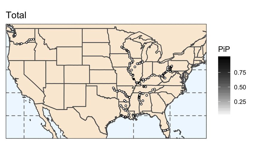
namely the Lock Performance Monitoring System (LPMS). The LPMS provides data on
tonnages moving through each of the 164 locks in the inland waterway system, essentially
providing 164 coincident variables that can be used to predict the eventual WBC release.5
      While the LPMS data provides a rich dataset to nowcast the WBC data, the large number
of variables provided in the LPMS presents a challenge for developing a nowcasting model
that incorporates these variables. When faced with such a large set of potential predictor
variables, there will exist substantial uncertainty over the correct set of variables to include
in the model. Specifically, in our application, there exists over 4.7 × 1049 potential models to
consider, where a model is defined as a particular set of predictor variables to include. One
approach to proceed in the face of this model uncertainty is to select a particular subset of
variables to include in the nowcasting model, perhaps through data-based methods. However,
this ignores relevant information contained in omitted variables. An alternative approach,
which would not omit information, is to simply include all potential predictor variables in the
nowcasting model. However, with a large number of variables, this approach will typically
lead to substantial estimation uncertainty, and thus inaccurate nowcasts. This is especially
the case when samples sizes are limited and/or variables are highly correlated. Further
complicating matters is that traffic shifts over the network through time may change the the
set of predictor variables best explaining the waterborne traffic data.
      Bayesian methods are attractive in settings that include significant model uncertainty, as
they provide a straightforward, intuitive, and consistent approach to measure and incorporate
model uncertainty when estimating parameters and constructing forecasts. BMA confronts
these issues by averaging forecasts produced by each candidate model included in the model
space. Averaging is accomplished using weights equal to the Bayesian posterior probability
that a particular model is the correct forecasting model. Thus, models that are deemed by
the data to be better forecasting models will receive higher weight in producing the BMA

5
    The LPMS data are recorded by the lockmaster for each of 164 locks and are readily available at
    https://corpslocks.usace.army.mil/
    They differ in mode of collection and what they record http://www.iwr.usace.army.mil/ndc/index.htm.

                                                    2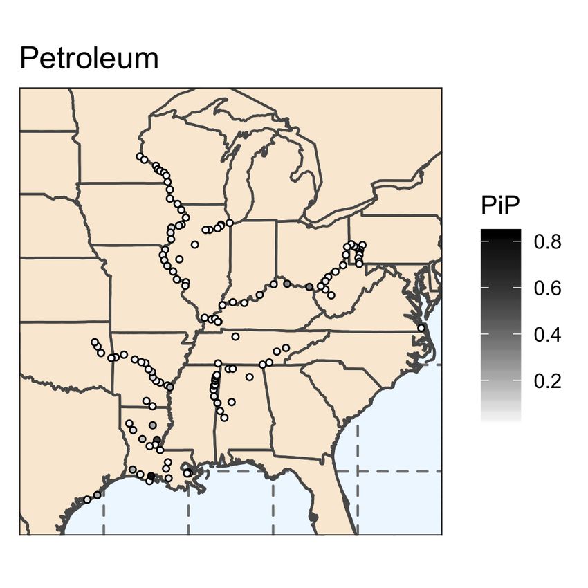
forecast. BMA also provides posterior inclusion probabilities for each explanatory variable,
a useful measure of which predictors provide the most relevant information for constructing
forecasts.
   In this paper, we adapt and apply these techniques to nowcast WBC tonnages in total and
for the four primary commodity groups in the United States. As potential predictor variables
we use the LMPS data for each of the 164 locks, as well as lags of macroeconomic variables.
We first provide in-sample estimation results constructed from data covering January 2000
to December 2013. These results demonstrate that there is substantial uncertainty regarding
which predictor variables belong in the true nowcasting model, as the model probabilities
are spread over a very large number of possible models. This provides empirical justification
of the use of BMA techniques in our setting. We then conduct an out-of-sample nowcasting
experiment extending from January 2011 to December 2013. To account for possible changes
in the composition of movements over the inland waterway network throughout time, we
re-estimate the models on a rolling window prior to forming each out-of-sample nowcast.
Our results suggest that the BMA procedure combined with the rolling-window estimation
provides very accurate nowcasts, improving substantially on the accuracy of existing studies
that produced nowcasts of waterborne commerce data.
   Our paper fits into a larger literature that explores forecasting and nowcasting transporta-
tion data. Babcock and Lu (2002) construct an ARIMAX model to explore the short-term
forecasting of inland waterway traffic using data for grain tonnage on the Mississippi River
and find their model provides accurate forecasts. Tang (2001) develops an ARMA model to
forecast quarterly variation for soybean and wheat tonnage on the McClellan-Kerr Arkansas
River. She finds that incorporating structural breaks into the model allows it to provide more
accurate forecasts. Thoma and Wilson (2004a) analyze shocks to barge quantities and rates
from changes in ocean freight rates, and rail rates and deliveries. The authors use vector
autoregressions and variance decompositions with an application to weekly transportation
data. Thoma and Wilson (2004b) estimate the co-integrating relationships between river

                                              3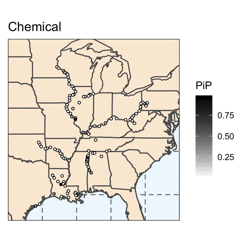
traffic, lock capacities, and a demand measure from 1953 through 2001. Forecasts of river
traffic are developed based on the co-integrating relationship over an extended period of time.
Thoma and Wilson (2005) explore the value of information contained in the LPMS data for
nowcasting WBC values. They use annual data to identify key locks with pair-wise corre-
lations and step-wise regressions, including these as predictors for annual WBC tonnages.
Our paper contributes to this literature by introducing BMA to forecasting transportation
networks.
    The remainder of the paper proceeds as follows. Section 2 describes the data and provides
an example of waterborne commerce movements. Section 3 outlines the general nowcast-
ing model and describes the Bayesian Model Averaging approach to construct nowcasts. In
Section 4 we present results regarding which predictor variables are most relevant for con-
structing nowcasts, as well as results from the out-of-sample nowcasting exercise. Finally,
Section 5 provides some discussion and concluding remarks.

2     Background

    In this section, we first describe the waterway system and the location of the lock system.
Figure 1 provides a map of the U.S. inland and intracoastal waterways system. This system’s
25,000 miles of navigable water directly serve 38 states and carries nearly one sixth of all
cargo moved between cities in the United States. The Gulf Coast ports of Mobile, New
Orleans, Baton Rouge, Houston, and Corpus Christi are connected to the major inland
ports of Memphis, St. Louis, Chicago, Minneapolis, Cincinnati, and Pittsburgh via the Gulf
Intracoastal Waterway and the Mississippi River. The Mississippi River is essential to both
domestic and foreign U.S, trade, allowing shipping to connect with barge traffic from Baton
Rouge to the Gulf of Mexico. The Columbia-Snake River System provides access from the
Pacific Northwest 465 miles inland to Lewiston, Idaho (Infrastructure Report Card, 2009).

                                               4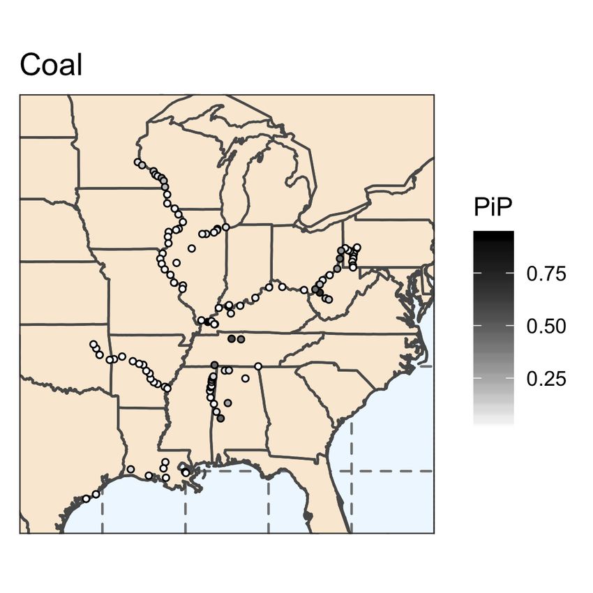
Figure 1
Inland and Intracoastal Waterways System
Source: Infrastructure Report Card
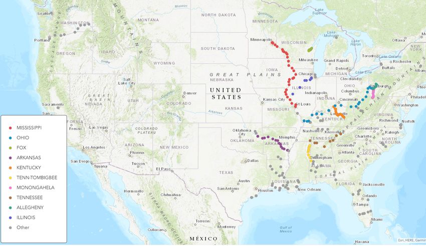
In Figure 2, we map the lock locations by river. As is evident in this figure, the locks
that comprise the LPMS are concentrated in the Midwest and Southeast regions of the
country. The majority of inland waterway commerce is concentrated along the Ohio River
and the Mississippi River. The various geographic origins of each commodity and changes in
demand for these commodities likely influence traffic patterns over time. Coal is the largest
commodity by volume transported along the inland waterway system but its role has been
declining as natural gas has become more attractive. The decline in demand for coal is likely
to influence traffic patterns, which could potentially impact which locks provide the most
valuable information in predicting WBC flows.
5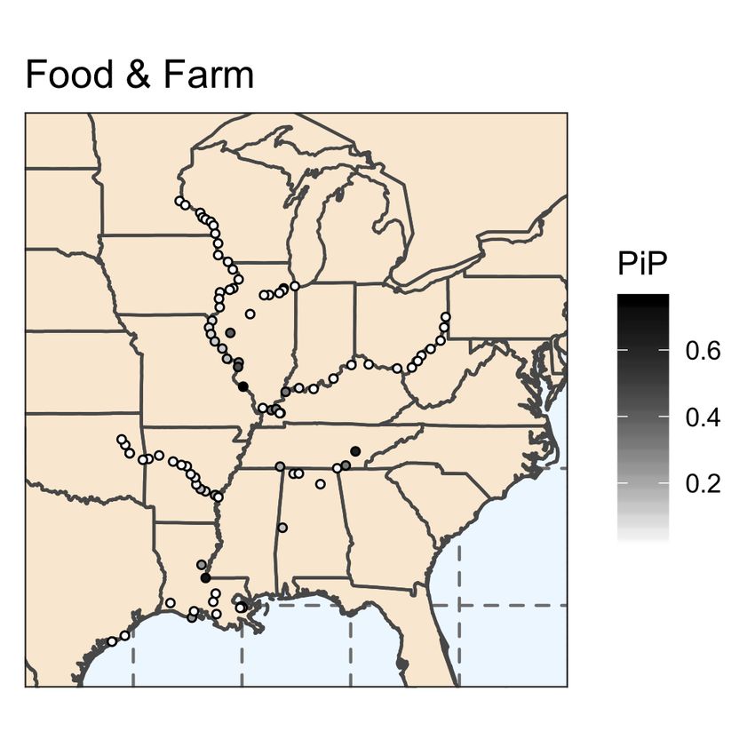
Figure 2
                                        Lock Location by River

2.1        Data

      We next describe the sources and characteristics of the Waterborne Commerce (WBC)
data and the Lock Performance Monitoring System (LPMS) data. The WBC data are
developed from monthly reports of waterway transportation suppliers, and measure the
tonnage by commodity group moved along the inland waterway system. Specifically, the
WBC data measures tons traveling on all US rivers measured in total (all commodities), as
well as for four commodity groups: food and farm product tons, coal tons, chemical tons,
and petroleum tons. There is substantial processing associated with the WBC data, and its
release time lags the data by a year or more. WBC data is highly accurate and is considered
the industry standard. In contrast, the LPMS data records tonnages of commodities passing
through specific inland locks, as recorded by the lock operator. It is available relatively
quickly, typically within a month (Navigation Data Center, 2013.)6 While the LPMS data

6
    Although the LPMS annual report in typically released in March, initial figures are made available on the
    US Army Corps website and can be accessed in real-time https://corpslocks.usace.army.mil/

                                                       6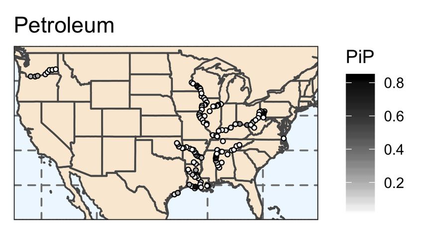
and the WBC data measure different quantities, they are very much connected as shown
below.
    The dependent variable in our analysis is defined as WBC tonnage (overall or by specific
commodity group) and is measured monthly for the years 2000-2013 as reported by the
Waterborne Commerce Statistics Center. The predictor variables include the LPMS lock
variables, provided by the Summary of Locks and Statistics, courtesy of the US Army Corps
of Engineers Navigation Data Center’s Key Lock Report. The report contains monthly total
tonnage values measured for 2000-2013 for each of 164 specific locks in the system. These
data were supplemented by employment statistics obtained from the US Bureau of Labor
Statistics which provides data at the national level for years 2000-2013. Specifically, we
include the two-month lag of the unemployment rate as an additional potential predictor.7
    In Figure 3, we present total commodity tonnage of the inland waterway network through-
out time. Specifically, this figure details annual LPMS tonnage for total commodities moving
along the two major rivers, the Mississippi and Ohio, as well as an Other category that ac-
counts for tonnage along the remaining 26 rivers.8 That is, the value for each river represents
the sum of all tonnages passing through all locks for a specific river. The fluctuations in
LPMS tonnage along the Mississippi River can be attributed to seasonal fluctuations in river
accessibility. Notice that the tonnages appear relatively stable.
    In Figure 4, we present commodity specific tonnage moving along the inland waterway
network. The Ohio River facilitates the majority of coal movement along the network,
accounting for 68% of all coal LPMS tonnage. The Mississippi River helps to distribute food
and farm products throughout the country, accounting for 57% of all food and farm LPMS
tonnage. Petroleum products tend to travel along the Gulf Intracoastal Waterway, with
43% of all petroleum products being transported through this system. Chemical tonnages
appear to be evenly distributed amongst the Mississippi River, the Ohio River, and the Gulf
7
  We follow the literature and include the second lag of the unemployment rate rather only. The LPMS data
  is available for a given month more quickly than the unemployment rate. Using the second lag ensures that
  use of the LPMS data to nowcast the WBC data is not held up by unemployment data.
8
  See Table 1 for a stylized example that relates the LPMS data to the WBC data.

                                                    7
Figure 3
LPMS Tonnage by River
  Total Commodities

       Figure 4
LPMS Tonnage by River
 Primary Commodities

          8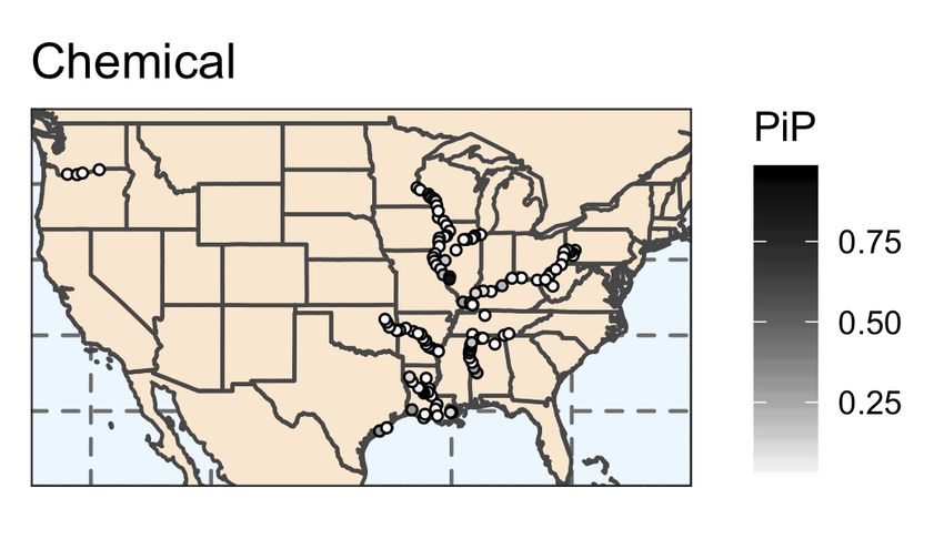
Intracoastal Waterway, with 74% of all chemical LPMS tonnage traveling along these three
rivers.

2.2       WBC via the LPMS

   This paper uses LPMS data as a coincident indicator for WBC data. The WBC data
are the result of firms filling out a monthly form, while the LPMS data are the result of
lockmasters recording the tonnages and commodities at each lock. To illustrate the two types
of data and how they are related, we follow Thoma and Wilson (2005) and present a stylized
example that relates the LPMS data to the WBC data. The example demonstrates that
changes in tonnages through key locks are useful for capturing changes in overall tonnages
moving on the river. To clarify the differences and connections of the LPMS and WBC data,
consider a river that has three locks labeled L1, L2, and L3. Suppose that during the time
period that tonnages are measured, there are four barge loads that move on the river. The
tonnages and movements between locks are:
                        Load   1 10 tons through    lock L1
                        Load   2 30 tons through    locks L1 and L2
                        Load   3 40 tons through    locks L1, L2, and L3
                        Load   4 20 tons through    locks L2 and L3

The WBC data measure the sum of all loads (in tons) moved on the river. Hence, the
WBC measurement is 10+30+40+20 = 100. The LPMS measurements reflect totals for
each individual lock. For example, Load 3 has a total of 40 tons that travel through L1,
L2, and L3. The LPMS data then records 40 tons for L1, 40 tons for L2, and 40 tons for
L3. In contrast, the WBC data records 40 tons. The final LPMS data for the four loads
described above is reported in Table 1. The idea is to use the LPMS variables to capture
changes in overall tonnage moving on the river by estimating a statistical model relating
WBC to LPMS variables. Simply including all LPMS variables when the number of such
variables is large is likely to be ineffective, as there will be substantial estimation uncertainty
associated with the weights that should be given to the individual locks. Also, some locks are

                                                9
likely uninformative (or redundant) for total tonnage, suggesting that a nowcasting model
should focus on a select group of key locks. Section 3 provides a more formal and consistent
treatment using Bayesian techniques to identify key locks.
Table 1
LPMS Data Example (tons)
Lock L1 L2 L3
Load 1 10
Load 2 30 30
Load 3 40 40 40
Load 4 20 20
Totals 80 90 60
3 Empirical Model and Bayesian Model Averaging
3.1 The Nowcasting Model
In this section, we present the nowcasting models used to predict WBC values given
LPMS data. We focus on linear candidate models that relate the WBC river tonnage in
month t to the second lag of the unemployment rate, and some subset of the 164 lock tonnage
variables provided by LPMS. Equation (1) below is an example of one of approximately
4.7 × 1049 such candidate models that we could consider:
W BCt = β0 + β1 U Rt−2 + β2 M I15t + β3 OH52t + εt (1)
εt ∼ i.i.d. N (0, σ 2 ).
In Equation (1), W BCt is the relevant WBC variable (total tonnage or commodity specific
tonnage) measured in month t, U Rt−2 is the second monthly lag of the U.S. unemployment
rate, M I15 is the total tons passing through lock 15 on the Mississippi River in month t,
and OH52 is the total tons passing through lock 52 on the Ohio River in month t. In this
example, there are thus two LPMS lock variables included in the model.
10Estimating this model provides a way to quantify the relationship between specific locks
and WBC flows. Note that although the left-hand side WBC variable and the right-hand
side LPMS lock variables are measured for the same period, the LPMS variables are available
far earlier than the WBC variable.9 With the LPMS data released prior to the corresponding
WBC data, the LPMS data serves as a coincident indicator to nowcast the WBC variables.
Equation (1) includes a specific subset of LPMS lock variables as predictors, and thus
represents one possible model that might be used to nowcast the WBC data using the LPMS
variables. One could simply include all possible lock variables in the model, but this would
lead to substantial estimation uncertainty and likely low quality forecasts. Indeed, for our
dataset, if all potential predictor variables were included in the nowcasting model there would
exist only three degrees of freedom, as we have 168 observations and 165 potential variables.
Estimation uncertainty is further exacerbated by the fact that many of the LPMS lock
variables are highly collinear. With only 168 observations, a parsimonious representation
of the data is of vital importance in order to preserve the statistical power of the nowcast.
However, exactly which representation should be used is unclear, meaning there is substantial
model uncertainty.
3.2 Bayesian Model Averaging
We consider linear regression models as in Equation (1), where the models differ by
the specific set of predictor variables included in the model. Again, these possible predictor
variables include the 164 LPMS lock variables and the unemployment rate. Label a particular
model as Mj , where a “model” consists of a choice of which variables to include in the linear
regression typified by Equation (1). Here, j = 1, 2, . . . , J and J is the number of possible
models. Again, as discussed above, J is approximately 4.7 × 1049 in our setting.
With such a large number of possible models, as well as our relatively small sample
size, there is significant uncertainty regarding the true model that should be used to form
9
The timing difference between the releases is variable and uncertain, but can be as long as 1.5 years.
11nowcasts. Here we take a Bayesian approach to compare and utilize alternative models.
Specifically, the Bayesian approach to compare alternative models is based on the posterior
probability that Mj is the true model:
f (Y |Mj ) P r(Mj )
P r(Mj |Y ) = J
, j = 1, ..., J (2)
P
f (Y |Mi ) P r(Mi )
i=1
where Y indicates the observed data, P r(Mj ) is the researcher’s prior probability that Mj
is the true model and f (Y |Mj ) is the marginal likelihood for model Mj :
Z
f (Y |Mj ) = f (Y |θj , Mj ) p(θj |Mj )dθj
where θj holds the parameters of the j th model, f (Y |θj , Mj ) is the likelihood function for
model Mj and p(θj |Mj ) is the prior density function for the parameters of Mj . In words,
the marginal likelihood function has the interpretation of the average value of the likelihood
function, and therefore the average fit of the model, over different parameter values. The
marginal likelihood plays an important role in Bayesian model comparison, as this term is
increasing in sample fit, but decreasing in the number of parameters estimated. This penalty
for more complex models naturally prevents overparameterization, an attractive feature for
developing a nowcasting model.
The posterior model probability P r(Mj |Y ) can be used to confront model uncertainty.
For example, one could select the model with highest posterior probability and then construct
nowcasts based on this best model alone. However, this focus on one chosen model ignores
potentially relevant information in models other than the chosen model. This is especially
important when the posterior model probability is dispersed widely across a large number of
models. Instead of basing inference on the single highest probability model, BMA proceeds
by averaging posterior inference regarding objects of interest across alternative models, where
averaging is with respect to posterior model probabilities. For example, suppose we have
12j
constructed a nowcast for W BCt from each model Mj , and we label these nowcasts W
\ BC t .
We can then construct a BMA nowcast as follows:
J
X j
W
\ BC t = W
\ BC t Pr(Mj |Y ) (3)
j=1
Another object of interest in this setting is the posterior inclusion probability, or P IP , for
a particular predictor variable. Specifically, suppose we are interested in whether a particular
predictor variable, labeled Xn , belongs in the true model. The P IP is constructed as:
J
X
P IPn = Pr(Mj |Y )Ij (Xn ) (4)
j=1
where Ij (Xn ) is an indicator function that is one if Xn is included in model Mj and zero
otherwise. In other words, the PIP for Xn is simply the sum of all the posterior model
probabilities for all models that include Xn . This PIP provides a useful summary measure
of which variables appear to be particularly important for nowcasting the WBC variable.
To implement the BMA procedure, we require two sets of prior distributions. The first
is the prior distribution for the parameters of each regression model. When the space of
potential models is very large, as is the case here, it is useful to use prior parameter densities
that are fully automatic, in that they are set in a formulaic way across alternative models.
To this end, we follow the strategy of (Fernández et al., 2001) for setting priors for the
parameters of linear regression models in BMA applications. These priors are designed for
the case where the researcher wishes to use as little subjective information in setting prior
densities as possible, and was shown by FLS to both have good theoretical properties and
perform well in simulations for the calculation of posterior model probabilities. Additional
details can be found in (Fernández et al., 2001).
The second prior distribution we require is the prior distribution across models, Pr(Mj ).
Here, we use a prior suggested in Ley and Steel (2009), which is uniform with respect to model
13size. In other words, models that include the same number of predictor variables receive the
same prior weight. Also, the group of all models that include a particular number of predictor
variables receives the same weight as the group of all models that contain a different number
of predictor variables. Further details can be found in Ley and Steel (2009.)
While conceptually straightforward, implementing BMA in our setting is complicated by
the enormous number of models under consideration. Specifically, the summation in the
denominator of Equation (2) includes so many elements as to be computationally infeasible.
To sidestep this difficulty we use the Markov-chain Monte Carlo Model Composition (M C 3 )
approach of Madigan and York (1993). M C 3 proceeds by constructing a Markov-chain Monte
Carlo sampler that produces draws of models from the multinomial probability distribution
defined by the posterior model probabilities. It is then possible to construct a simulation-
consistent estimate of P r(Mj |Y ) as the proportion of the random draws for which model
Mj was drawn. For our implementation of M C 3 we use one million draws from the model
space, following 100,000 draws to ensure convergence of the Markov-chain based sampler.
We implement a variety of standard checks to ensure the adequacy of the number of pre-
convergence draws.10
4 Results
4.1 In-Sample Variable Inclusion Results
BMA constructs nowcasts as an average across models with different sets of predictors.
To better understand the set of predictors and which are most useful in nowcasting WBC
values, we apply BMA to the full sample of data extending from January 2000 to December
2013. In Table 2, we report the top 10 models ranked by posterior model probability, both
for the case where the dependent variable is total WBC tonnage and for the cases where the
dependent variable is a specific commodity type. As Table 2 makes clear, these top 10 models
10
A textbook treatment of the M C 3 algorithm can be found in Koop (2003.)
14account for less than 2% of the total posterior model probability for all possible models.
This suggests that the posterior model probability is spread across a very large number of
models, highlighting the significant model uncertainty associated with our dataset. This
also highlights the importance of the BMA approach, in that it incorporates the information
contained in all models, rather than focusing on any single model that receives low posterior
model probability.
Table 2
Posterior Model Probabilities for Top 10 Models
Pr(Mj |Y )
Total Coal Farm Petro Chem
1 1.47 1.72 1.31 1.61 1.57
2 1.42 1.28 1.20 1.49 1.28
3 1.12 1.17 1.17 1.23 1.17
4 1.11 0.96 1.15 1.09 1.01
5 0.95 0.95 0.99 1.05 0.98
6 0.82 0.82 0.93 0.96 0.94
7 0.81 0.83 0.92 0.73 0.86
8 0.80 0.80 0.86 0.65 0.82
9 0.77 0.70 0.75 0.63 0.69
10 0.75 0.67 0.72 0.58 0.68
Note: Posterior model probabilities for top 10 highest probability models. All table
entries should be multiplied by 10−7
Given the empirical relevance of BMA, we next present the PIPs in order to evaluate
which locks appear most important for nowcasting WBC. The PIPs are calculated as in
Equation (4). Figures 5 and 6 displays the PIPs for total WBC tonnage in two different ways.
In Figure 5 the PIPs are presented via a map, where we focus on the main inland waterway
network.11 In Figure 6, we present the posterior inclusion probability for all predictors via
a bar chart. The horizontal axis displays each explanatory variable while the vertical axis
measures the posterior inclusion probability. The explanatory variables are too voluminous
to represent in the figure; however, the ordering follows the river names (Allegheny, Atlantic
Intercoastal Waterway, Atchafalaya, Blackwarrior Tombigbee, Calcasieu, Chicago, Canaveral
11
The full map is presented in the Appendix Figure 11.
15Harbor, Columbia, Cumberland, Freshwater Bayou, Green and Barren, Gulf Intracoastal
Waterway, Illinois Waterway, Kanawha, Kaskaskia, Mississippi, Mc-Kerr Arkansas River
Navigation System, Monongahela, Ouachita and Black, Old, Ohio, Okeechobee Waterway,
Red, St. Marys, Snake, Tennessee, Tennessee Tombigbee Waterway) and lock number, with
the final predictor representing the two-month lag unemployment rate. As two examples,
the predictor with the largest posterior inclusion probability in Figure 6 corresponds to the
Kaskaskia River Navigation Lock (PIP = 0.9995), while the predictor with the second largest
posterior inclusion probability corresponds to the Barkley Lock (PIP = 0.8099). This means
that out of the models sampled by M C 3 , the Kaskaskia Lock appeared as a predictor in over
99% of these models.
The results reveal that there exist several explanatory variables that have a high prob-
ability of being included in the true nowcasting model; however, the majority of locks have
less than a 5% probability of being included in the model. This figure again highlights the
advantage of the BMA approach relative to methods that select a particular model. All po-
tential explanatory variables have a non-zero posterior inclusion probability, indicating that
all explanatory variables appear in the nowcast. Out of the 1,000,000 draws taken as part of
the M C 3 algorithm, the average model contains 14 explanatory variables. Hence, BMA is
able to directly incorporate all explanatory variables into the nowcast, while also preserving
statistical power. In Table 3, we list the explanatory variables with the largest posterior
inclusion probabilities. This table highlights the locks that help to predict WBC flows in
total commodities. Of the 165 predictors considered, the BMA approach picks up eight locks
that appear in at least half of the models sampled by M C 3 . Note that the Kaskaskia River
Navigation Lock has a posterior inclusion probability of 0.9995, which means that this lock
appeared in over 99% of the models sampled by M C 3 . This result is not surprising, as this
lock is located in the free-flowing area of the Middle Mississippi River. That is, unlike the
Upper Mississippi, which contains a series of locks and dams, the Middle Mississippi only
contains this single lock. Additionally, the Middle Mississippi connects waterborne com-
16merce between the Upper Mississippi and the Ohio River, the two largest river systems by
volume. Hence, any waterborne commerce traveling between the Mississippi River and the
Ohio River must travel through and be recorded in the LPMS tonnage of the Kaskaskia
River Navigation Lock.
Figure 5
Posterior Inclusion Probability
In Figure 7, we display the commodity specific posterior inclusion probabilities for locks
in the inland waterway network.12 In Figure 8, we present the commodity specific poste-
rior inclusion probabilities for all predictors. The predictive ability of each lock varies by
commodity, as expected due to the geographic variation in waterway routes. Similar to the
results for total commodities, commodity specific posterior inclusion probabilities reveal sub-
stantial model uncertainty. For each commodity, there exist several locks that have a high
probability of being included in the model; however, the majority of locks have less than a
12
The full map is presented in Appendix Figure 12.
17Figure 6
Posterior Inclusion Probability
Table 3
BMA Results - Total
Explanatory Variable PIP River
Kaskaskia River Navigation Lock 0.9995 Kaskaskia
Barkley Lock 0.8099 Cumberland
Racine Locks and Dam 0.7675 Ohio
Smithland Lock and Dam 0.6383 Ohio
Willow Island Locks and Dam 0.6187 Ohio
Calcasieu Lock 0.5982 Gulf
Cheatham Lock 0.5510 Cumberland
John T. Meyers Lock and Dam 0.5098 Ohio
Note: Results for the explanatory variables with PIP > 0.5.
185% probability of being included in the commodity specific model. Similar to the results for
total commodities, commodity specific posterior inclusion probabilities for all explanatory
variables are non-zero, revealing that all explanatory variables appear in the nowcast for
each commodity.
Figure 7
Posterior Inclusion Probability
19Figure 8
Posterior Inclusion Probability
In Table 4, we present the commodity specific BMA results for the explanatory vari-
ables with posterior inclusion probabilities greater than 0.5. For each commodity, there
exist different sets of locks that provide superior predictive ability. Note that the chemical
results reveal a posterior inclusion probability of 0.9885 for the two-month lag unemploy-
ment rate, which means this variable appeared in over 98% of the models sampled by M C 3 ,
providing evidence that the unemployment rate contains valuable information in predicting
contemporaneous and future chemical WBC flows.
20Table 4
BMA Results - Primary Commodities
Commodity Explanatory Variable PIP River
Coal Lock and Dam 52 0.9261 Ohio
Coal Winfield Locks and Dam Main 1 0.6804 Kanawha
Coal Cheatham Lock 0.5787 Cumberland
Food & Farm Kaskaskia River Navigation Lock 0.7489 Kaskaskia
Food & Farm Old River Lock 0.6725 Old
Food & Farm Watts Bar Lock 0.6221 Tennessee
Petroleum Inner Harbor Navigation Canal Lock 0.8312 Gulf
Petroleum Leland Bowman Lock 0.7830 Gulf
Petroleum Lock and Dam 3 0.7126 Monongahela
Petroleum Colorado River East Lock 0.5985 Gulf
Petroleum Jonesville Lock and Dam 0.5605 Ouachita
Chemical Unemployment Rate (two-month lag) 0.9885
Chemical John H. Overton 0.9619 Red
Chemical Chain of Rocks Lock and Dam 27 0.8814 Mississippi
Chemical Colorado River East Lock 0.6580 Gulf
Note: Results for the explanatory variables with PIP > 0.5.
4.2 Out-of-Sample Nowcast Results
This section provides results of an out-of-sample nowcast experiment using our BMA
approach. To account for possible changes in the composition of movements over the inland
waterway network throughout time, we re-estimate the models on a rolling window prior
to forming each out-of-sample nowcast. That is, the model is estimated using data from
January 2000 to January 2010 and then a BMA nowcast for January 2000 is constructed.
Next, the model is re-estimated using data from February 2000 to February 2010 and then
a nowcast for February 2000 is constructed. This process is repeated until we have nowcasts
through December 2013.
Figure 9 visualizes the out-of-sample nowcast accuracy of the BMA approach for total
WBC tonnage. This plot shows the WBC data relative to the WBC nowcast values for total
commodities. Figure 10 visualizes the out-of-sample nowcast accuracy of the BMA approach
for specific commodities. These plots show the WBC data relative to the WBC nowcast
values for each commodity. The BMA approach is able to predict close to the actual tonnage
21for total and for all primary commodities. The M C 3 algorithm is capable of providing
accurate nowcasts while avoiding the problems associated with an overparameterized model.
Figure 9
Comparison of Actual WBC Tons to Nowcast WBC Tons
Here, we present a summary measure of how well the BMA procedure performed at
estimating the true WBC values at each point in time. Specifically, Table 5 provides the
mean squared error (M SE) for each commodity and Table 6 provides the average percentage
forecast error for each commodity. The M SE for the nowcast is calculated by:
T
X 1 \
M SE = (W BC t − W BCt )2 (5)
t=1
T
where W
\ BC t is the BMA nowcast of W BCt defined in Equation (3). The results indicate
that the WBC values were estimated accurately by the BMA approach, with the largest
M SE being 356.27, and all commodity specific M SE below 56.97.13 Based on these nowcast
evaluation metrics, we conclude that the LPMS data provides the most value for predicting
contemporaneous values of chemical tonnage, where all M SE are below 8.66. These translate
13
For M SE, we scale the units to hundreds of thousands of tons.
22into average percentage forecast errors of less than 2.4% for total, 1.3% for coal, 5.7% for
food and farm, 2.2% for petroleum, and 4.8% for chemical tonnages.
Figure 10
Comparison of Actual WBC Tons to Nowcast WBC Tons
(Millions of Tons)
Table 5
Nowcast Evaluation Metrics - M SE
Year Total Coal Farm Petroleum Chemical
2010 257.76 19.67 46.87 56.94 8.66
2011 356.27 55.73 33.59 43.21 8.45
2012 228.02 32.08 35.79 37.00 5.60
2013 166.20 7.54 28.74 20.00 2.50
Note: Hundreds of thousands of tons.
23Table 6
Average Percentage Forecast Error
Year Total Coal Farm Petroleum Chemical
2010 1.98 -0.65 3.23 -0.94 4.75
2011 -2.31 -0.27 2.29 -2.13 2.95
2012 -0.34 0.28 1.08 -1.44 1.02
2013 -0.96 -1.23 -5.69 1.45 -1.27
5 Concluding Remarks
This paper develops an estimation technique to nowcast WBC data based on a coin-
cident indicator of LPMS and unemployment data. Nowcasts are averaged across models
with different sets of predictors. The results indicate that the LPMS and unemployment
data provide valuable information in predicting contemporaneous WBC values, and that a
model averaging approach to nowcasting waterborne commerce can substantially increase
predictive performance. Benchmark priors provide a data-based method of sifting through
and downweighing less relevant explanatory variables. The BMA technique included all po-
tential predictors in each commodity specific nowcast while maintaining sufficient degrees of
freedom. Hence, BMA helped to alleviate the problems associated with an overparameter-
ized model while also preserving statistical power. This approach provides a consistent way
of incorporating both model and parameter uncertainty.
Historically, nowcasts of waterway traffic were impeded by issues of variable selection and
changes in traffic patterns. BMA with M C 3 overcomes these issues by sampling the model
space and constructing nowcasts that contain highly informative predictors. Individual locks
that signal WBC flows are included in producing nowcasts, while excluding locks that contain
too much noise. Implementing the nowcast with a rolling window helps to incorporate issues
arising from changes in traffic patterns. Leveraging the LPMS and unemployment data
to predict contemporaneous and future WBC values provide both market participants and
24government policy makers useful information earlier than if they wait for the release of the
actual data.
The BMA approach is limited by computational resources and the quality of available
data. Market participants and government policy makers interested in quantifying model
uncertainty, without prior knowledge of the predictive ability of their covariates, can set
benchmark priors and let the data drive the results. This approach can be generalized to
wide data sets (N < K) that lack the statistical power necessary to conduct valid inference.
Future areas of application may include long-run forecasts of transport demand, where the
periodicity and structure of the data tend to dictate the set of feasible and appropriate
estimation techniques.
25Appendix
Figure 11
Posterior Inclusion Probability
Figure 12
Posterior Inclusion Probability
26References
American Society of Civil Engineers. (2009) “Infrastructure Report Card.”
American Society of Civil Engineers. (2017) “Infrastructure Report Card.”
Armstrong, J. Scott. (1985) “Long-range Forecasting.” John Wiley and Sons Inc..
Babcok, Michael and Xiaohua Lu. (2002) “Forecasting Inland Waterway Grain Traffic.”
Transportation Research Part E: Logistics and Transportation Review, 38: 65-74.
Berge, Travis J.. (2015) “Predicting Recessions with Leading Indicators: Model Averaging
and Selection Over the Business Cycle.” Journal of Forecasting, 34(6): 455-471.
Blonigen, Bruce A. and Jeremy Piger. (2014) “Determinants of Foreign Direct Investment.”
Canadian Journal of Economics, 47(3): 775-812.
Fernández, Carmen and Eduardo Ley and Mark F. J. Steel. (2001) “Model Uncertainty in
Cross-Country Growth Regressions.” Journal of Applied Econometrics, 16(5): 563-576.
Hastings, W.K. (1970). Monte Carlo sampling methods using Markov chains and their ap-
plications. Biometrika. 57, 97-109.
Koop, Gary. (2003) “Bayesian Econometrics.” John Wiley and Sons Inc., Bayesian Model
Averaging, 265-280.
Navigation Data Center. (2013) “Lock Performance Monitoring System Key Lock Report.”
US Army Corps of Engineers.
Owyang, Michael T. and Jeremy Piger and Howard J. Wall. (2015) “Forecasting National
Recessions Using State-level Data.” Journal of Money, Credit and Banking, 47(5): 847-866.
Roberts, G.O., Gelman, A., Gilks, W.R. (1997). “Weak Convergence and Optimal Scaling
of Random Walk Metropolis Algorithms.” Ann. Appl. Probab. 7, 110-20.
Tang, Xiuli. (2001) “Time Series Forecasting of Quarterly Barge Grain Tonnage on the
McClellan-Kerr Arkansas River Navigation System.” Journal of Transportation Research
Forum, 43: 91-108.
Thoma, Mark A.. (2008) “Structural change and lag length in VAR models.”
Thoma, Mark A. and Wesley W. Wilson. (2004a) “Market Adjustments Over Transportation
Networks: A Time Series Analysis of Grain Movements on the Inland Waterway System.”
27Institute for Water Resources, Technical Report, US Army Corps of Engineers.
Thoma, Mark A. and Wesley W. Wilson. (2004b) “Long-run Forecasts of River Traffic on
the Inland Waterway System.” Institute for Water Resources, Technical Report, US Army
Corps of Engineers.
Thoma, Mark A. and Wesley W. Wilson. (2005) “Leading Transportation Indicators: Fore-
casting Waterborne Commerce Statistics Using Lock Performance Data.” Journal of Trans-
portation Research Forum, 44(2).
Transportation Research Board. (2015) “Funding and Managing the US Inland Waterways
System.” The National Academies of Sciences, Engineering, and Medicine.
Sims, Chris A. and James H. Stock and Mark W. Watson. (2002) “Inference in Linear Time
Series Models with Some Unit Roots.” Econometrica, 58: 113-144.
Stock, James H. and Mark W. Watson. (2002) “Macroeconomic Forecasting Using Diffusion
Indexes.” Journal of Business & Economic Statistics, 20(2): 147-162.
U.S. Bureau of Labor Statistics, Civilian Unemployment Rate [UNRATENSA], retrieved
from FRED, Federal Reserve Bank of St. Louis; https://fred.stlouisfed.org/series/UNRATENSA,
February 8, 2019.
Waterborne Commerce Statistics Center. (2013) “Waterborne Commerce of the United
States.” Institute for Water Resources.
Zivot, E., and J. Wang. “Modeling Financial Time Series with S PLUS. 2nd ed. NY:
Springer Science+Business Media, Inc., 2006.
28You can also read