"Regional Climate Model Emulator Based on Deep Learning: Concept and First Evaluation of a Novel Hybrid Downscaling Approach" - 1233 July 2021 ...
←
→
Page content transcription
If your browser does not render page correctly, please read the page content below
1233

                                                  July 2021

“Regional Climate Model Emulator Based on Deep Learning:
Concept and First Evaluation of a Novel Hybrid Downscaling
                        Approach”

      Lola Corre, Antoine Doury, Sébastien Gadat, Aurélien Ribes
                          and Samuel Somot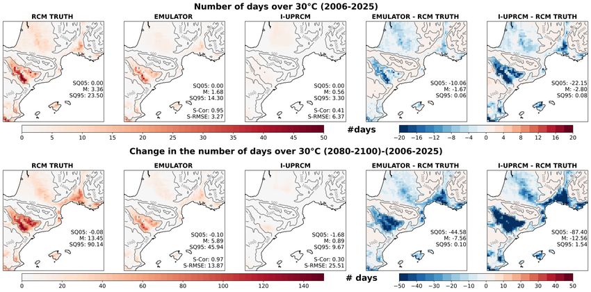
Regional Climate Model emulator based on deep
learning: concept and first evaluation of a novel
hybrid downscaling approach

Antoine Doury(1) · Samuel Somot(1) ·
Sebastien Gadat(2) · Aurélien Ribes(1) ·
Lola Corre(3)

Received: date / Accepted: date

Abstract Providing reliable information on climate change at local scale re-
mains a challenge of first importance for impact studies and policymakers.
Here, we propose a novel hybrid downscaling method combining the strengths
of both empirical statistical downscaling methods and Regional Climate Mod-
els (RCMs). The aim of this tool is to enlarge the size of high-resolution RCM
simulation ensembles at low cost.
We build a statistical RCM-emulator by estimating the downscaling function
included in the RCM. This framework allows us to learn the relationship be-
tween large-scale predictors and a local surface variable of interest over the
RCM domain in present and future climate. Furthermore, the emulator relies
on a neural network architecture, which grants computational efficiency.
The RCM-emulator developed in this study is trained to produce daily maps
of the near-surface temperature at the RCM resolution (12km). The emulator
demonstrates an excellent ability to reproduce the complex spatial structure
and daily variability simulated by the RCM and in particular the way the RCM
refines locally the low-resolution climate patterns. Training in future climate
appears to be a key feature of our emulator. Moreover, there is a huge compu-
tational benefit in running the emulator rather than the RCM, since training
the emulator takes about 2 hours on GPU, and the prediction is nearly in-
stantaneous.
However, further work is needed to improve the way the RCM-emulator re-
produces some of the temperature extremes, the intensity of climate change,
and to extend the proposed methodology to different regions, GCMs, RCMs,
and variables of interest.
Antoine Doury
(1) CNRM, Université de Toulouse, Météo-France, CNRS, Toulouse, France
(2) Toulouse School of Economics, Université Toulouse 1 Capitole, Institut Universitaire de

France
(3) Météo-France, Toulouse, France

Tel.: +33561079104
E-mail: antoine.doury@meteo.fr
2                                                  Antoine Doury(1) et al.

Keywords Emulator · Hybrid downscaling · Regional Climate Modeling ·
Statistical Downscaling · Deep Neural Network · Machine Learning

4                                                                                                                        Antoine Doury(1) et al.

Contents

1   Introduction . . . . . . .   .   .   .   .   .   .   .   .   .   .   .   .   .   .   .   .   .   .   .   .   .   .   .   .   .   .   .   .   .   .   .   .   .    5
2   Methodology . . . . . .      .   .   .   .   .   .   .   .   .   .   .   .   .   .   .   .   .   .   .   .   .   .   .   .   .   .   .   .   .   .   .   .   .    8
3   Results . . . . . . . . .    .   .   .   .   .   .   .   .   .   .   .   .   .   .   .   .   .   .   .   .   .   .   .   .   .   .   .   .   .   .   .   .   .   19
4   Discussion . . . . . . .     .   .   .   .   .   .   .   .   .   .   .   .   .   .   .   .   .   .   .   .   .   .   .   .   .   .   .   .   .   .   .   .   .   27
5   Conclusion . . . . . . .     .   .   .   .   .   .   .   .   .   .   .   .   .   .   .   .   .   .   .   .   .   .   .   .   .   .   .   .   .   .   .   .   .   34
6   Acknowledgement . . .        .   .   .   .   .   .   .   .   .   .   .   .   .   .   .   .   .   .   .   .   .   .   .   .   .   .   .   .   .   .   .   .   .   36
7   Supplementary material       .   .   .   .   .   .   .   .   .   .   .   .   .   .   .   .   .   .   .   .   .   .   .   .   .   .   .   .   .   .   .   .   .   37
Title Suppressed Due to Excessive Length                                       5

1 Introduction

    Climate models are an essential tool to study possible evolutions of the
climate according to different scenarios of greenhouse gas emissions. These
numerical models represent the physical and dynamical processes present in
the atmosphere and their interactions with other components of the Earth
System. The complexity of these models involves compromises between the
computational costs, the horizontal resolution and, in some cases, the domain
size.

    Global Climate Models (GCMs) produce simulations covering the whole
planet at reasonable cost thanks to a low spatial resolution (from 50 to 300
km). The large number of different GCMs developed worldwide allows to build
large and coordinated ensembles of simulations, thanks to a strong interna-
tional cooperation. These big ensembles (CMIP3/5/6, Meehl et al, 2007; Taylor
et al, 2012; Eyring et al, 2016) are necessary to correctly explore the different
sources of variability and uncertainties in order to deliver reliable information
about future climate change at large spatial scales. However, the resolution of
these models is too coarse to derive any fine scale information, which is of pri-
mary importance for impact studies and adaptation policies. Consequently, it
is crucial to downscale the GCM outputs to a higher resolution. Two families
of downscaling have emerged: empirical-statistical downscaling and dynamical
downscaling. Both approaches have their own strengths and weaknesses.

    Empirical Statistical Downscaling methods (ESD) estimate functions to
link large scale atmosphere fields with local scale variables using observational
data. Local implications of future climate changes are then obtained by ap-
plying these functions to GCM outputs. Gutiérrez et al (2019) present an
overview of the different ESD methods and evaluate their ability to downscale
historical GCM simulations. The great advantage of these statistical methods
is their computational efficiency, which makes the downscaling of large GCM
ensembles possible. On the other hand, they have two main limitations due to
their dependency on observational data. First of all, they are applicable only
for regions and variables for which local long-term observations are available.
Secondly, they rely on the stationary assumption of the large-scale / local-scale
relationship, which implies that a statistical model calibrated in the past and
present climate remains reliable in the forthcoming climate. Studies tend to
show that the calibration period has a non-negligible impact on the results
(Wilby et al, 1998; Schmith, 2008; Dayon et al, 2015; Erlandsen et al, 2020).

   Dynamical Downscaling (DD) is based on Regional Climate Models (RCMs).
These models have higher resolution than GCMs (1 to 50 km) but are restricted
to a limited area domain to keep their computational costs affordable. They
are nested in a GCM, e.g., they receive at small and regular time intervals
dynamical information from this GCM at their lateral boundaries. One key
advantage of RCMs is to rely on the same physical hypotheses as the one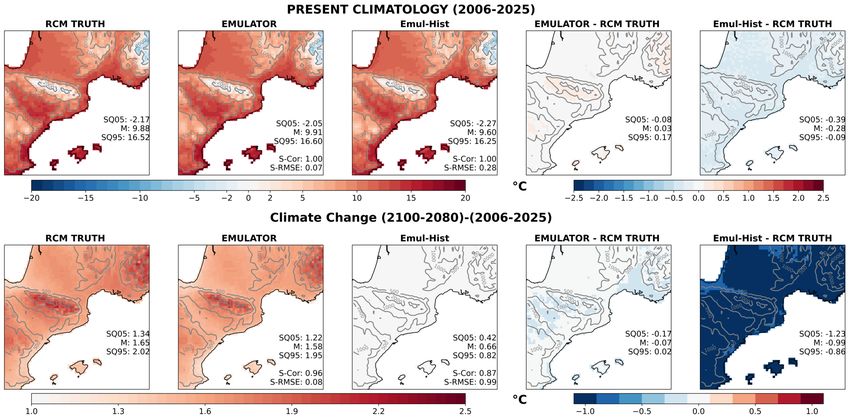
6                                                          Antoine Doury(1) et al.

involved in GCMs. They provide a complete description of the state of the
atmosphere over their domain through a large set of variables at high tempo-
ral and spatial resolution. The added value of RCMs has been demonstrated
in several studies (Giorgi et al, 2016; Torma et al, 2015; Prein et al, 2016;
Fantini et al, 2018; Kotlarski et al, 2015, for examples). In order to deliver
robust information about future local responses to climate change, it is nec-
essary to explore the uncertainty associated with RCM simulations. Déqué
et al (2007) and Evin et al (2021) assess that four sources of uncertainty are
at play in a regional climate simulation: the choice of the driving GCM, the
greenhouse gas scenario, the choice of the RCM itself and the internal vari-
ability. Their relative importance depends on the considered variables, spa-
tial scale, and timeline. According to these results, it is important (Déqué
et al, 2012; Evin et al, 2021; Fernández et al, 2019) to complete 4D matrices
[SCEN ARIO, GCM, RCM, M EM BERS] to deliver robust messages, where
members are several simulations of each (SCEN ARIO, GCM, RCM ) triplet.
However, the main limitation of RCM is their high computational costs, and
completion of such matrices is impossible.

    This study proposes a novel hybrid downscaling method to enlarge the size
of RCM simulation ensembles. The idea is to combine the advantages of both
dynamical and statistical downscaling to tackle their respective limits. This
statistical RCM-emulator uses machine learning methods to learn the relation-
ship between large scale fields and local scale variables inside regional climate
simulations. It aims to estimate the downscaling function included in the RCM
in order to apply it to new GCM simulations. This framework will allow to
learn this function on the entire RCM domain, in past and future climate,
under different scenarios. Besides, the emulator relies on Machine Learning
algorithms with low computational costs, which will enable to increase RCM
simulation ensembles and to better explore the uncertainties associated with
these high resolution simulations.

    Hybrid statistical-dynamical downscaling methods have already been pro-
posed. They are methods which combine, in different ways, regional climate
models and statistical approaches to obtain local climate information. Several
studies such as Pryor and Barthelmie (2014), Vrac et al (2012) or Turco et al
(2011) perform 2-step downscaling by applying ESD methods to RCM simu-
lations. Colette et al (2012) apply bias correction methods to GCM outputs
before downscaling with RCMs. Maraun and Widmann (2018) are among the
first to mention the concept of emulators. Few studies have combined ESD and
DD for the same purpose as in this study. For instance, Walton et al (2015)
propose a statistical model which estimates from GCM outputs, the high res-
olution warming pattern for each month in California. It is calibrated using
RCM simulations and relies on a simple linear combination of two predictors
from the GCM (the monthly mean over the domain and an indicator for the
land/sea contrast) plus an indicator for the spatial variance (obtained thanks
to PCA). Berg et al (2015) adapt the same protocol for monthly changes in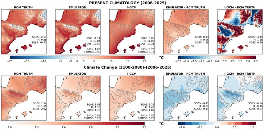
Title Suppressed Due to Excessive Length                                      7

precipitation over California. With respect to those pioneer studies, we pro-
pose here to further develop this approach by using a neural network based
method and by emulating the full time series at the input time scale, allowing
to explore daily climate extremes.

    In recent years, climate science has taken advantage of the recent strides
in performances of Deep Learning algorithms (see Lecun et al, 2015, for an
overview). Indeed, thanks to their capacity to deal with large amounts of data
and the strong ability of Convolutional Neural Network (CNN) (LeCun et al,
1998) to extract high level features from images, these algorithms are particu-
larly adapted to climate and weather sciences. Reichstein et al (2019) present
a complete overview of the climate studies applying Deep Learning and future
possibilities. In particular, Vandal et al (2019) and Baño-Medina et al (2020,
2021) showed a good ability of convolutional neural network architecture to
learn the transfer function between large scale fields and local variables in
statistical downscaling applications. The concept of emulator is mentioned in
Reichstein et al (2019) as surrogate models trained to replace a complex and
computationally expensive physical model (entirely or only parts of it). Once
trained, this emulator should be able to produce simulations much faster than
the original model. In this context, the RCM-emulator proposed here is based
on a different fully convolutional neural network architecture known as UNET
(Ronneberger et al, 2015).

    This study presents and validates the concept of statistical RCM-emulator.
We will focus on emulating the near-surface temperature in a RCM over a spe-
cific domain, including high mountains, shore areas, and islands in Western
Europe. This domain regroups areas where the RCM presents added value
compared to GCM but remains small enough to perform quick sensitivity
tests. This paper is organized as follows: Section 2 presents the whole frame-
work to define, train and evaluate the emulator, while Section 3 shows the
emulator results. Finally, Sections 4 and 5 discuss the results of the emulator
and provide conclusions.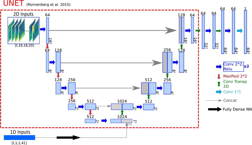
8                                                                    Antoine Doury(1) et al.

                                  Table 1: Notations

    Notation            Description                             Dimensions
                     Spatial indexes over
    i, j                                                 {i, j} ∈ [[1 , I]] × [[1 , J]]
                          input grid
                     Spatial indexes over
    k, l                                                 {k, l} ∈ [[1 , K]] × [[1 , L]]
                         target grid
    t               Temporal index, daily                          t∈N
    x                2-D variables index                List of 2D Variables : V 2D
    z                1-D variables index                List of 1D Variables : V 1D
                       Set of 2D input
    X                                            Xt,i,j,x ∈ {N × [[1 , I]] × [[1 , J]] × V 2D}
                      for the emulator
                       Set of 1D input
    Z                                                          Zt,z {N × V 1D}
                      for the emulator
                        Target : Daily
    Y                                                 Yt,k,l ∈ {N × [[1 , K]] × [[1 , L]]}
                  Near-Surface Temperature
    F          Downscaling function of the RCM
    F̂           Emulator : Estimation of F

2 Methodology

    This section provides a complete description of the RCM-emulator used
in this paper. The notations are summarised in Table 1. The RCM-emulator
uses a neural network architecture to learn the relationship between large-
scale fields and local-scale variables inside regional climate simulations. RCMs
include a downscaling function (F) which transforms large scale information
(X,Z) into high resolution surface variables (Y). The statistical RCM-emulator
aims to solve a common Machine Learning problem

                                     Y = F (X, Z)

which is to estimate F by F̂ in order to apply it to new GCM simulations.
The following paragraphs describe the list of predictors used as inputs and
their domain, the predictand (or target) and its domain, the neural network
architecture, the framework used to train the emulator and the metrics used
to evaluate its performances.

2.1 Models and simulations

    This study focuses on the emulation of the daily near-surface temperature
from EURO-CORDEX simulations based on the CNRM-ALADIN63 regional
climate model (Nabat et al, 2020) driven by the CNRM-CM5 global climate
model used in CMIP5 (Voldoire et al, 2013). The latter provides lateral bound-
ary conditions, namely 3D atmospheric forcing at 6-hourly frequency, as well
as sea surface temperature, sea ice cover and aerosol optical depth at monthly
frequency. The simulations use a Lambert Conformal grid covering the Euro-
pean domain (EUR-11 CORDEX) at the 0,11◦ (about 12.5 km) scale (Jacob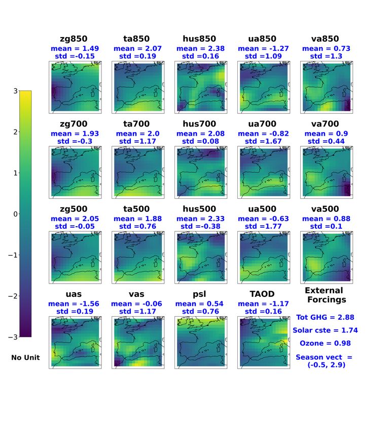
Title Suppressed Due to Excessive Length                                                         9

                                   Table 2: List of predictors

                                                      2D Variables
         Field              Altitude Levels      Variables Notation   Units   Temporal Aggregation   Dimension
                                                        zg500
      Geopotential          850 , 700, 500 hPa          zg700          m           Daily mean          [i, j]
                                                        zg850
                                                       hus500
   Specific Humidity         850 , 700, 500 hPa         hus700                      Daily mean          [i, j]
                                                       hus850
                                                        ta500
      Temperature           850 , 700, 500 hPa          ta700          K           Daily mean          [i, j]
                                                        ta850
                                                       ua500
                            850 , 700, 500 hPa
                                                       ua700
    Eastward Wind                   +                                 m/s          Daily mean          [i, j]
                                                       ua850
                                  Surface
                                                         uas
                                                        va500
                            850 , 700, 500 hPa
                                                        va700
   Northward Wind                   +                                 m/s          Daily mean          [i, j]
                                                        va850
                                  Surface
                                                         vas
  Sea Level Pressure             Surface                 psl           Pa          Daily mean          [i, j]
 Total Aerosol Optical
                                                       TAOD                       Monthly mean         [i, j]
    Depth forcing
                                                      1-D Variables
  Daily spatial means                                    x
                                                                                     Daily            [#V 2D]
    of 2D variables                                with x ∈ V 2D
 Daily spatial standard                                   •
       deviation                                          x
                                                                                     Daily            [#V 2D]
    of 2D variables                                 with x ∈ V 2D
 Total Anthropogenic
    greenhouses gas                                    ant ghg                       Yearly             [1]
        forcings
   Solar and Ozone
                                                       sol, oz                       Yearly             [2]
        forcings
  Seasonal Indicators
       2πt          2πt                                cos,sin                       Daily              [2]
  Cos( 365 ) ; Sin( 365 )

et al, 2014). The historical period runs from 1951 to 2005. The scenarios (2006-
2100) are based on two Representative Concentration Pathways from the fifth
phase of the Coupled Model Intercomparison Project (CMIP5): RCP4.5 and
RCP8.5 (Moss et al, 2010). The monthly aerosol forcing evolves according to
the chosen RCP and the driving GCM.

2.2 Predictors

    Neural Networks can deal with large datasets at low computational time.
During their self optimisation, they are able to select the important variables
and regions for the prediction. In this way, a large number of raw predictors
can be given to the learning algorithm, with minimum prior selection (which
could introduce some bias) or statistical pre-work (which might delete some
of the information). Several ESD studies (Lemus-Canovas and Brands, 2020;
Erlandsen et al, 2020) show that the right combination of predictors depends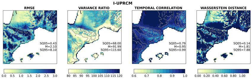
10                                                              Antoine Doury(1) et al.

strongly on the target region and the season. The RCM domains are often
composed of very different regions in terms of orography, land types, distance
to the sea, etc. For these reasons, we decided to give all potentially needed
predictors to the emulator and leave the algorithm to determine the right
combination to be used to predict each RCM grid point.

    The set of predictors (X, Z) used as input in the emulator is composed
of 2 dimensional variables X, and 1D predictors Z (Table 2). The set of 2D
variables includes atmospheric fields commonly used in ESD (Baño-Medina
et al, 2020; Gutiérrez et al, 2019) at different pressure levels. We also added
the total aerosol optical depth present in the atmosphere since it constitutes
a key regional driver of the regional climate change over Europe (Boé et al,
2020). It leads 20 2D predictors. These variables are normalised (see Equation
1) according to their daily spatial mean and standard deviation so that they
all have the same importance for the neural network before the training.

    The set of 1D variables includes external forcing also given to the RCM:
the total concentration of greenhouse gases and the solar and ozone forcings.
It also includes a cosinus, sinus vector to encode the information about the
day of the year. Given that the 2D variables are normalised at each time step
by their spatial mean, they don’t carry any temporal information. For this
reason, the daily spatial means and standard deviations time series for each
2D variable are included in the 1D input, bringing the size of this vector to 43.
In order to always give normalised inputs to the emulator, Z is normalized (see
Equation 2 ) according to the means and standard deviations over a reference
period (1971-2000 here) chosen during the emulator training. The same set of
means and standard deviations will be used to normalise any low resolution
data to be downscaled by the emulator.

    This decomposition of the large scale information consists in giving sepa-
rately the spatial structure of the atmosphere (X) and the temporal informa-
tion (Z) to the emulator. Thanks to the neural network architecture described
in Section 2.4.3, we force the emulator to consider both items of information
equally.

                             X�t,i,j,x = Xt,i,j,x − X t,x                          (1)
                                                 •
                                               Xt,x
                                                   �
                     �I �                          ��
                          J                        � I �  J
                             Xt,i,j,x              �        (X       − X t,x )2
                     i=1 j=1                •      � i=1 j=1 t,i,j,x
      with X t,x   =                  and Xt,x =
                          I ×J                                I ×J
Title Suppressed Due to Excessive Length 11
Zt,z − Z ref,z
Z�t,z = • (2)
Z ref,z
� ��
�
Zt,z � (Z − Z ref,z )2
t∈R • � t∈R t,z
with Z ref,z = and Zref,z =
nb days in R nb days in R
where R is the reference period.
The aim of the emulator is to downscale GCM simulations. Klaver et al
(2020) shows that the effective resolution of climate models is often larger
(about 3 times) than its nominal resolution. For instance, CNRM-CM5 can-
not be trusted at its own horizontal resolution (≈ 150 km) but at a coarser
resolution, probably about 450 to 600 km. For this reason, the set of 2D pre-
dictors are smoothed with a 3 × 3 moving average filter. The grid of the GCM
is conserved, with each point containing a smoother information than the raw
model outputs.
For this study the input domain is defined around the target domain (de-
scribed in Section 2.3). It is a 16 × 16 ( J = I = 16 in Table 1) CNRM-CM5
grid box visible on Figure 1. Each observation given to the emulator (see Fig-
ure 1 for an illustration) is a day t and it is composed of a 3D array (Xi,j,x ),
where the two first dimensions are the spatial coordinates and the third di-
mension lists the different variables chosen as predictors, and a 1D array (Zz )
regrouping all the 1 dimensional inputs.
2.3 Predictands
In this study, to assess the ability of the RCM-emulator to reproduce the
RCM downscaling function, we focused on the emulation of the daily near
surface temperature over a small but complex domain. The target domain
for this study is a box of 64x64 RCM grid points at 12km resolution (about
600 000 km2 ) centred over the south of France (Figure 1). It gathers different
areas of interest for the regional climate models. It includes three mountain
massif (Pyrenees, Massif Central and French Alps) which are almost invisible
at the GCM scale (specially the Pyrenees). The domain also includes coastlines
on the Mediterranean side and on the Atlantic side. Thanks to a better repre-
sentation of the coastline at the RCM resolution, it takes better into account
the sea effect on the shore climate. It was also important for us to add small
islands on our evaluation domain, such as the Baleares (Spain), since they
are invisible on the GCM grid and the RCM brings important information.
Finally, three major rivers (plotted in blue in Figure 1) are on the domain
with interesting impacts on climate (commented in Section 3): the Ebro in
Spain, the Garonne in southwest of France and the Rhone on the east of the
domain. This domain should therefore illustrate the added value brought by
a RCM at local scale and be a good test-bed on the feasibility of emulating12 Antoine Doury(1) et al.
ee
( X , Z )t
Yt
F
t = 1st August 2000
Fig. 1: Illustration of an observation. Left: each map represents a 2D input
variables (X), on the input domain, and the blue numbers correspond to the
1D variables (Z). Right: an example of Y , the near surface temperature on
the target domain.
high resolution models.
2.4 Deep learning with UNET
2.4.1 Neural network model as a black-box regression model
The problem of statistical downscaling and of emulation of daily near-
surface variables may be seen as a statistical regression problem where we
need to build the best relationship between the output response Y and the
input variables (X, Z). When looking at the L2 loss between the prediction Ŷ
and the true Y , the optimal link (denoted by F below) is theoretically known
as the conditional expectation:
F (X, Z) = E[Y |(X, Z)].
Unfortunately, since we will only have access to a limited amount of observa-
tions collected over a finite number of days, we shall work with a training setTitle Suppressed Due to Excessive Length 13
formed by the collected observations ((Xt , Zt ), Yt )1≤t≤T and try to build from
the data an empirical estimation F� of the unknown F .
For this purpose, we consider a family of relationship between (X, Z) and
Y generated by a parametric deep neural network, whose architecture and
main parameters are described later on. We use the symbol θ to refer to the
values that describe the mechanism of one deep neural network, and Θ as
the set of all possible values of θ. Hence, the family of possible relationships
described by a collection of neural networks correspond to a large set (Fθ )θ∈Θ .
Deep learning then corresponds to the minimization of a L2 data-fidelity term
associated to the collected observations:
T
�
F̂ = arg min �Yt − Fθ (Xt , Zt )�2 . (3)
Fθ ,θ∈Θ
t=1
2.4.2 Training a deep neural network
To train our emulator between low resolution fields and one high resolution
target variable, we used a neural network architecture called UNET whose
architecture is described below. As usual in neural networks, the neurons of
UNET are organised in layers. Given a set En of input variables denoted by
(xi )i∈En of an individual neuron n, the output of n corresponds to a non-linear
transformation φ (called activation function) of a weighted sum of its inputs:
n ((xi )i∈En ) = φ (�w, (xi )i∈En �) .
The connection between the different layers and their neurons then depends
on the architecture of the network. In a fully connected network (multilayer
perceptron) all the neurons of a hidden layer are connected to all the neurons
of the previous layer. The deepness of a network then depends on the number
of layers.
As indicated in the previous paragraph, the machine learning procedure
corresponds to the choice of a particular set of weights over each neuron to
optimise a data fidelity term. Given a training set, a deep learning algorithm
then solves a difficult multimodal minimisation problem as the one stated in
(3) with the help of gradient descent strategies with stochastic algorithms. The
weights associated with each neuron and each connection are then re-evaluated
according to the evolution of the loss function, following the backpropagation
algorithm Rumelhart and Hinton (1986). This operation is repeated over all
the examples until the error is stabilized. Once the neural network is trained,
it may be used for prediction, i.e., to infer the value Y from new inputs (X, Z).
We emphasize that the bigger the dimension of the inputs and outputs,
the larger the number of the parameters to be estimated and so the bigger
the training set must be. Therefore, the quality of the training set is crucial:
missing or wrong values will generate some additional fluctuation and errors in14 Antoine Doury(1) et al.
the training process. Moreover, we also need to cover a sufficiently large variety
of scenarios in the input variables to ensure that our training set covers a wide
range of possible inputs. For all these reasons, climate simulation datasets are
ideal to train deep learning networks.
2.4.3 UNET architecture
UNET is a specific network architecture that has been introduced in Ron-
neberger et al (2015) for its good abilities in image segmentation problems,
which consists in identifying different objects and areas in an image. This in-
colves at gathering pixels that correspond to the same object. This key feature
is of course naturally interesting for meteorological maps since the emulator
needs to identify the different meteorological structures present in the low res-
olution predictors for a given day, in order to produce the corresponding high
resolution near-surface temperature.
UNET is a fully convolutional neural network (LeCun et al, 1998), as it is
composed only of convolutional layers. A convolutional layer applies different
moving filters to the input images in order to decompose them in a set of
features. The user choose the size of the filters and their number. This feature’s
extraction allows the network to decompose images in many features in order
to identify the relevant part for the target prediction.
From a technical point of view, the original UNET (Ronneberger et al,
2015) is composed of two paths: the contracting one (also called encoder)
and the expansive one (decoder). Figure 2 represents the UNET architecture
scheme used in this study. It contains a cascade of standard steps of convolu-
tional neural networks, that are described below. The different layers used in
the network are:
– Each blue arrow ⇒ corresponds to a convolution block composed of a layer
built with a set of convolutional 2×2 filters. The number of filters increases
all along the contracting part (the number of filters is respectively 64, 128,
256, 512 and 1024 and is given on the top of each block in Figure 2). The
outputs of this layer are then normalised with a batch normalisation layer
(see e.g. Ioffe and Szegedy (2015)) to improve the statistical robustness of
the layer. Finally the ReLu activation function completes this block.
ReLu : R(z) = max(0, z)
�
– Each red arrow � is a Maxpooling layer. It performs 2 × 2 pooling on each
feature map, which simply divides by 2 the spatial dimension by taking the
maximum of each 2 × 2 block. It is applied through all convolution block
outputs in the encoding path. The size of the images is indicated on the
side of each block �
on Figure 2.
– Each green arrow � is a transpose convolution layer. It allows to perform
up-sampling in the expansive part of the algorithm. It multiplies the spatial
dimension by 2 by applying the same connection as the classical convolution
but in the backward direction.Title Suppressed Due to Excessive Length 15
– The black arrow =⇒ represents a fully connected dense network of 4 layers
which is applied on the 1-dimensional inputs (Z).
– The grey arrow ⇒ represents a simple concatenation layer which recalls
the layers from the encoding path in the decoding one.
– Finally, the light blue arrow ⇒ is the output layer, which is a simple con-
volutional layer with a single filter and a linear activation function.
The Unet proposed here takes the same basis as the original one but en-
larges the expansive path by a succession of up-sampling layers in order to
reach target size (Figure 2). Moreover, the Unet architecture allowed us to
add a 1-dimensional input (see Section 2.2 on Predictors) at the bottom of the
“U” after a short fully dense network of 4 layers. At this point the neural net-
work concatenates the encoded spatial information (from X) and the encoded
temporal information (from Z). As illustrated in Figure 2 we force the Unet to
give the same importance to these 2 inputs before starting the decoding path
and recreating the high resolution temperature map.
We chose the Mean Square Error (MSE) as the loss function to train the
network, as we are in a regression problem. Moreover, it is well adapted for
variables following gaussian-like distribution such as temperature. The neural
network was built and trained using the Keras Tensorflow environment in
Python (https://keras.io). The network trained for this study has about 25
billion parameters to fit.
2.5 Training of the emulator : Perfect Model Framework
As any statistical downscaling and any machine learning method, the em-
ulator needs to be calibrated on a training set. It consists in showing the em-
ulator many examples of predictors and their corresponding target such that
the parameters of the network can be fitted as mentioned in Section 2.4.2.
The emulator is trained in a perfect model framework, with both predictors
and predictands coming from the same RCM simulation. The intuitive path to
train the emulator is to use GCM outputs as predictors and its driven RCM
outputs as predictands, but there are many reasons for our choice. First of all,
it guarantees a perfect temporal correlation between large scale predictors and
a local scale predictand. Indeed, Figure 3 shows that GCM and RCM large
scales are not always well correlated, with an average correlation of 0.9 and
10% of the days with a coefficient of correlation lower than 0.75. These mis-
matches are quite well known and often due to internal variability as explained
by Sanchez-Gomez et al (2009); Sanchez-Gomez and Somot (2018). Moreover,
there are more consistent biases (discussed in Section 4.1) between GCM and
RCM large scales. It is of primary importance that the inputs and outputs
used to calibrate the model are perfectly consistent, otherwise, the emulator
will try to learn a non-existing or non-exact relationship. In this context, the
perfect model framework allows us to focus on the downscaling function of the
RCM, specifically.16 Antoine Doury(1) et al.
...
Fig. 2: Scheme of the neural network architecture used for this paper. The
part of the network in the red frame corresponds to the original unet defined
in Ronneberger et al (2015)
The training protocol is summarised in Figure 4a. In a first step, the RCM
simulation outputs are upscaled to the GCM resolution (about 150km) thanks
to a conservative interpolation. This first step transforms the RCM outputs
into GCM-like outputs. This upscaled RCM is called UPRCM in the rest of
this paper. In the second step, these UPRCM outputs are smoothed by a 3x3
moving average filter to respect the protocol described in Section 2.2. This
smoothing also ensures to delete local scale information which might persist
through the upscaling.
The near-surface temperature on the target domain is extracted from the same
RCM simulation. Following this procedure, the emulator is trained using the
ALADIN63 simulation forced by CNRM-CM5, covering the 1950-2100 period
with the RCP8.5 scenario from 2006. We chose the two most extreme simula-
tions (historical and RCP8.5) for the training in order to most effectively cover
the range of possible climate states since the emulator does not target to ex-
trapolate any information. Future studies could explore the best combination
of simulations to calibrate the emulator.Title Suppressed Due to Excessive Length 17
�����������������������������������������������������������������������������������
����
����
����
����
����
����
����
���� ���� ���� ���� ����
Fig. 3: Time series of spatial correlation of the atmospheric temperature at
700hpa between ALADIN63 and its driving GCM, CNRM-CM5, over the input
domain.
TRAINING EVALUATION STEP 1 EVALUATION STEP 2
RCM SIMULATION (0.11°) RCM SIMULATION (0.11°) GCM SIMULATION (1.4°) RCM
ALADIN 63, forced by CNRM-CM5, 1950-2100, RCP85 ALADIN 63, forced by CNRM-CM5, 2006-2100, RCP45 CNRM-CM5, 2006-2100, RCP45 SIMULATION
(0.11°)
Selection of 2D inputs Selection of 2D inputs ALADIN63
(X) Extraction of land (X) Selection of 2D inputs
Conservative interpolation Near Surface Conservative interpolation Y (X) Y
to 1.4° grid Temperature to 1.4° grid
Moving average filter
TAS
Moving average filter Moving average filter
Normalisation &
Normalisation & Normalisation & Comparison Extraction of 1D inputs (Z) Comparison
Extraction of 1D inputs (Z) Extraction of 1D inputs (Z)
ee
( X, Z ) EMUL-UNET Y
ee
( X, Z ) EMUL-UNET Y
ee
( X, Z ) EMUL-UNET Y
Fig. 4: Scheme of the protocols for the training (a) and the two steps of eval-
uations (b and c).
2.6 Evaluation metrics
The emulated temperature series (Ŷ ) will be compared to the original
RCM series (Y ) (mentioned as “RCM truth” in the rest of this paper) through
statistical scores described below. Each of these metrics will be computed in
each point over the complete series:
– RMSE. The Root Mean Squared Error measures the standard deviation
of the prediction error (in ◦ C):
�
� 1�
RM SE(Y, Y ) = (Yt − Y�t )2
T t
– Temporal Anomalies Correlation.This is the Pearson correlation co-
efficient after removing the seasonal cycle:
ACC(Y, Y� ) = ρ(Ya , Y
�a ),
with ρ the Pearson correlation coefficient and Ya and Y �a are the anomaly
series after removing a seasonal cycle computed on the whole series.18 Antoine Doury(1) et al.
– Ratio of Variance. It indicates the performance of the emulator in repro-
ducing the local daily variability. We provide this score as a percentage.
V ar(Y� )
RoV (Y, Y� ) = ∗ 100
V ar(Y )
– Wasserstein distance. It measures the distance between two probability
density functions (P, Q). It relies on the optimal transport theory (Villani,
2009) and measures the minimum required “energy” to transform P into
Q. The energy here corresponds to the amount of distribution weight that
is needed to be moved multiplied by the distance it has to be moved. In
this study we use the 1-d Wasserstein distance, and its formulation between
two samples becomes a rather simple function of ordered statistics:
T
�
W1 (f (Y ), f (Y� )) = �
|Y(i) − Y (i) |
i=1
with f (•) the probability density function associated with the sample •.
– Climatology. We compare the climatology maps over present (2006-2025)
and future (2081-2100, not shown in Section 3) climate. The RCM truth
and emulator maps are shown with their spatial correlation and RMSE.
The error (emulator minus RCM) map is also computed.
– Number of days over 30◦ C. Same as climatology for the maps showing
the number of days over 30◦ C.
– 99th Percentile. Same as climatology for the maps showing the 99th
percentile of the daily distribution.
– Climate Change. Climate change maps for the climatology, the number
of days over 30◦ C and the 99th percentile (delta between future (2080-2100)
and present (2006-2100) period).
These metrics are at the grid point scale and are presented as maps. How-
ever, to summarise these maps with few numbers we can compute their means
and their super-quantile of order 0.05 (SQ05) and 0.95 (SQ95). The super-
quantile α is defined as the mean of all the values larger (resp. smaller) than
the quantile of order α, when α is larger (resp. smaller) than 0.5. These values
are shown in the Figures of Section 3 and Tables 3 and 4 in supplementary
material.
2.7 Benchmark
For this study, we propose as benchmark the near surface temperature
from the input simulation (before the moving average smoothing), interpo-
lated on the target grid by bilinear interpolation. As this study is the first to
propose such an emulator, there is no already established benchmark. The one
proposed here is a naive high-resolution prediction given available predictors
(low-resolution). It allows the reader to locate the emulator somewhere in be-
tween the simplest possible downscaling (simple interpolation) and the mostTitle Suppressed Due to Excessive Length 19
complex one (RCM). All the metrics introduced in Section 2.6 will be applied
to our benchmark.
3 Results
This section presents the emulator performances in terms of its compu-
tational costs (in Section 3.1) and its ability to reproduce the near surface
temperature time series at high resolution. As illustrated in Figure 4, we will
evaluate the emulator in two steps, (1) in the perfect model world (Section
3.2) and (2) when the emulator inputs come from a GCM simulation (Section
3.3). The RCM simulation used to evaluate the model (also called target sim-
ulation) is the ALADIN63, RCP45, 2006-2100 forced by the GCM simulation
CNRM-CM5, RCP45, 2006-2100. Note that the emulator never saw the tar-
get simulation during the training phase. This evaluation exercise illustrates
a potential use of the emulator: downscaling a scenario that the RCM has not
previously downscaled.
3.1 Computational efficiency
The emulator is trained on a GPU (GeForce GTX 1080 Ti). About 60
epochs are necessary to train the network, and each epoch takes about 130
seconds with a batch size of 100 observations. The training of the emulator
takes about 2 hours. Once the emulator is trained, the downscaling of a new
low resolution simulation is almost instantaneous (less than a minute). It is a
significant gain in time compared to RCM, even if these time lengths do not
include the preparation of the inputs, which depends mainly on the size of the
series to downscale and on the data accessibility. It would, when including the
input preparation, take only a few hours on a simple CPU or GPU to produce
a simulation with the trained emulator, while it takes several weeks to perform
a RCM simulation on a super-computer.
3.2 Evaluation step 1 : Perfect model world
In a first step, the emulator is evaluated in the perfect model world, mean-
ing that the inputs come from the UPRCM simulation. This first evaluation
step is necessary to control the performances of the emulator in similar con-
ditions as during its training. Moreover, the perfect model framework guar-
antees perfect temporal matches between the large scale low resolution fields
(the inputs) and the local scale high resolution temperature (the target). The
emulator should then be able to reproduce perfectly the temperature series
that is simulated by the RCM. The benchmark for this first evaluation is the
UPRCM near surface temperature re-interpolated on the RCM grid. It is re-
ferred as “I-UPRCM”.20 Antoine Doury(1) et al.
(a)
(b)
Fig. 5: Randomly chosen illustration of the production of the emulator with
inputs coming from UPRCM: (a) temperature (◦ C) at a random day over the
target domain for the RCM truth, emulator, interpolated UPRCM, and (b)
random year time series (◦ C) for 4 particular grid points.
Figure 5a illustrates the production of the emulator for a random day re-
garding the target and the benchmark. The RCM truth map presents a refined
and complex spatial structure largely missing in the UPRCM map. Moreover,
it is evident on the I-UPRCM map that the simple bilinear interpolation does
not recreate these high resolution spatial patterns. The emulator shows for
this given day an excellent ability to reproduce the spatial structure of the
RCM truth. It has very accurate spatial correlation and RMSE and estimates
the right temperature range. On Figure 5b, we show the daily time series
for four specific points shown on the RCM truth map (Marseille, Toulouse, a
high Pyrenees grid point and a point in Majorca) during a random year. TheTitle Suppressed Due to Excessive Length 21
(a)
(b)
(c)
Fig. 6: (a) Daily probability density functions from the RCM truth, the emu-
lator and the I-UPRCM at 4 particular grid points over the whole simulation
period. (b) (resp. (c)) Maps of performance scores of the emulator (resp. of the
I-UPRCM) with respect to the RCM truth computed over the whole simula-
tion period. For each map, the values of the spatial mean and super-quantiles
(SQ05 and SQ95) are added.22 Antoine Doury(1) et al.
(a)
(b)
(c)
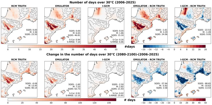
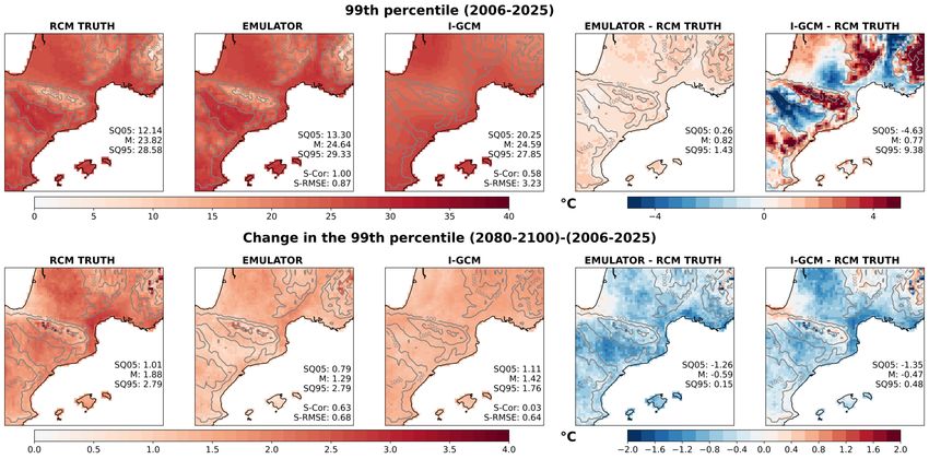
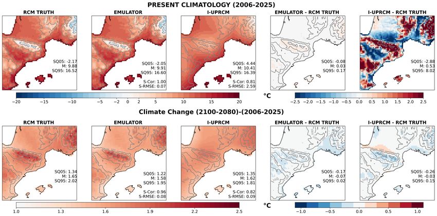
Fig. 7: (a) Maps of long-term mean climatologies, (b) number of days over
30◦ C and (c) 99th percentile of daily near-surface temperature for a present-
climate period (2006-2025) and for the climate change signal (2080-2100 minus
2006-2025), for the RCM truth, the emulator and the I-UPRCM. On each line,
the two last maps show the error map of the emulator and the I-UPRCM. For
each map, the spatial mean and super-quantiles (SQ05 and SQ95) are added,
as well as the spatial correlation and spatial RMSE for the emulator and I-
UPRCM maps.Title Suppressed Due to Excessive Length 23
RCM transforms the large scale temperature (visible on I-UPRCM) differently
over the four points. In the Pyrenees, the RCM shifts the series and seems to
increase the variance. In Marseille, it appears to produce a warmer summer
without strongly impacting winter characteristics, and it seems to be the exact
opposite in Majorca. On the contrary, in Toulouse, I-UPRCM and RCM are
close. For each of these 4 cases, the emulator reproduces the sophistication of
the RCM series almost perfectly.
Figure 5a gives the impression that the emulator has a good ability to
reproduce the complex spatial structure brought by the RCM, and we can
generalise this result with the other figures. First of all, the spatial correlation
(equal to 1) and the very low spatial RMSE (0.07◦ C) of the climatology maps
in Figure 7 in the present climate confirm that this good representation of the
temperature’s spatial structure is robust when averaging over long periods. In
particular, it is worth noting that the altitude dependency is well reproduced
as well as the warmer patterns in the Ebro and Rhone valley or along the
coastlines. The performance scores (Figure 6b) of the emulator support this
result. Their spatial homogeneity tends to show that the emulator does not
have particular difficulties over complex areas. Moreover, the comparison with
the interpolated UPRCM shows the added-value of the emulator and in par-
ticular its ability to reinvent the fine-scale spatial pattern of the RCM truth
from the large-scale field. Indeed, the score maps of the I-UPRCM (Figure 6c)
or the present climatology error map shows strong spatial structures, high-
lighting the regions where the RCM brings added value and that the emulator
reproduces successfully.
The RCM resolution also allows to have a better representation of the daily
variability at the local scales over critical regions. The difference in variance
between the I-UPRCM and the RCM is visible on Figure 6c. The I-UPRCM
underestimates the variability and is poorly correlated over the higher reliefs,
the coastlines and the river valley. In contrast, the emulator reproduces more
than 90% of the RCM variance over the whole domain. The RMSE and tem-
poral correlation maps of the emulator confirm the impression given by Figure
5b that it sticks almost perfectly to the RCM truth series. Moreover, the RCM
daily variability is strongly dependent on the region. Indeed, the RCM trans-
forms the “I-UPRCM” pdfs in different ways across the domain (visible on
Figures 6ac). Figures 6ab show that the emulator succeeds particularly well in
filling these gaps.
The emulator’s good representation of the daily variability and temporal
correlation involves a good representation of the extreme values. The proba-
bility density functions of the four specific points on Figure 6a show that the
entire pdfs are fully recreated, including the tails. The Wasserstein distance
map extends this result to the whole target domain. The two extreme scores
computed for the present climate on Figure 7bc confirm these results. The
99th percentile emulated map is almost identical to the target one verified24 Antoine Doury(1) et al.
by the difference map, with a maximum difference of less than 1◦ C for val-
ues over 35◦ C. The spatial pattern of the 99th percentile map is here again
correctly captured by the emulator, particularly along the Garonne river that
concentrates high extremes. The number of days over 30◦ C is a relatively more
complicated score to reproduce since it involves an arbitrary threshold. The
emulator keeps performing well with a high spatial correlation between the
emulator and the RCM truth. However, it appears that the emulator misses
some extreme days, involving a lack in the intensity of some extremes.
Finally, the high-resolution RCM produces relevant small-scale structures
in the climate change maps. In particular, RCMs simulate an elevation-dependent
warming (see the Pyrenées and Alps areas Kotlarski et al, 2015), a weaker
warming near the coasts (see the Spanish or Atlantic coast) and a specific
signal over the islands as shown in the second lines of Figures 7ac. It can be
asked if the emulator can reproduce these local specificities for the climate
change signal. The emulator is able to capture this spatial structure of the
warming but with a slight lack of intensity which is general over the whole
domain. The reproduction of the climate change in the extremes suffers the
same underestimation of the warming but also offers the same good ability to
reproduce the spatial structure, with high spatial correlation.
This first evaluation step shows that if the emulator is still perfectible, in
particular when looking at extremes or climate change intensity, it is able to
almost perfectly reproduce the spatial structure and daily variability of the
near surface temperature in the perfect model world.
3.3 Evaluation step 2 : GCM world
In this second evaluation step, we directly donwscale a GCM simulation
that has not been downscaled by the RCM. The benchmark for this evalua-
tion is the near surface temperature from the GCM, interpolated on the target
grid. It will be referred to as I-GCM. The emulated series and the benchmark
are compared to the RCM simulation driven by the same GCM simulation.
Figure 8a illustrates the production of the emulator regarding the bench-
mark and RCM truth for the same day as Figure 5a. First of all, as for the
I-UPRCM, the I-GCM map does not show any of the complex RCM spatial
structures. The I-GCM is less correlated with the RCM and warmer than the
I-UPRCM. In contrast, the emulator reproduces the complex spatial structure
of the RCM very well with a spatial correlation of 0.98 but appears to have
a warm bias with respect to the RCM truth. The four time series are consis-
tent with the previous section, with fundamental differences between I-GCM
and RCM, which the emulator captured very well. However, the correlation
between the emulator and the RCM seems to be not as good as in the perfectTitle Suppressed Due to Excessive Length 25
model framework.
Figure 8b is a very good illustration of the RCM-GCM large scale de-
correlation issue presented in Section 2.4.2. Indeed the less good correlation
of the emulator with the RCM is probably due to mismatches between GCM
and RCM large scales. For instance,in the beginning of November, on the time
series shown on Figure 8b, the RCM seems to simulate a cold extreme on
the whole domain, which appears neither in the interpolated GCM nor in the
emulator. The same kind of phenomenon occurs regularly along the series and
is confirmed by lower temporal correlations between the RCM truth and the
I-GCM (Figure 9c) than with the I-UPRCM (Figure 6c). According to this,
the emulated series can not present a good temporal correlation with the RCM
truth since it is a daily downscaling of the GCM large scale. Keeping in mind
these inconsistencies, it is still possible to analyse the performances of the em-
ulator if we leave aside these scores which are influenced by the poor temporal
correlation (RMSE, ACC).
As in the first step of the evaluation (Section 3.2), the spatial structure
of the RCM truth is well reproduced by the emulator. The present climatol-
ogy map (Figure 10a) has a perfect spatial correlation with the RCM. The
added value from the emulator is clear if compared to the interpolated GCM.
The spatial temperature gradients simulated by the GCM seem to be mainly
driven by the distance to the sea. On the other hand, the emulator manages
to recreate the complex structures created by the RCM, related to relief and
coastlines. The emulator capacity to reproduce the RCM spatial structure
seems as good as in Section 3.2. The scores in Figure 9b present a good spatial
homogeneity, exactly like in the previous section 6b.
The error map in Figure 10(a) shows that the emulator is warmer in the
present climate than the RCM truth (+0.96◦ C). This bias presents a North-
South gradient with greater differences over the North of the target domain,
which is consistent with the Wasserstein distance map on Figure 9b. The
Wasserstein metric shows that the density probability functions from the em-
ulated series are further away from the RCM truth with GCM-inputs than
in UPRCM mode. The similarities between the Wasserstein scores and the
present climatology difference map indicate that the emulator shifts the mean.
The daily variability is well reproduced by the emulator. As mentioned
before, the weaker RMSE (Figure 9b) is mainly due to the lower correlation
between GCM and RCM. But the ratio of variance demonstrates that the em-
ulator manages to reproduce the daily variability over the whole domain. The
RCM brings a complex structure of this variability (higher variability in the
mountains than in plains, for example), and the emulator, as in the first eval-
uation step, recreates this fine scale. Moreover, the daily pdfs of the emulator
(Figure 9a) are very consistent with the RCM ones, and the same range of26 Antoine Doury(1) et al.
values is covered for each of the four particular points.
This good representation of daily variability tends to suggest that the em-
ulator can reproduce the local extremes. Figures 10bc confirm these results,
with a very high spatial correlation between the emulator and the RCM truth
maps in present climate. The warmer extremes along the three river valleys
are present in both RCM and emulator maps, while they are absent from the
I-GCM maps. The warm bias observed in the present climatology map also
impacts these scores. The emulator map of the number of days over 30◦ C in
the present climate shows more hot days than the RCM but the same spatial
structure. The map of the 99th percentile over the 2006-2025 period shows the
same observation, with a warm bias (+0.82) slightly lower than the climatol-
ogy bias.
Finally, the climate change signal is also well captured by the emulator.
The different spatial patterns that bring the high resolution of the RCM in
the Figures 10abc are also visible in the emulator climate change Figures. The
emulator represents a weaker warming than the RCM, observable in average
warming but also on the map of extremes. This underestimated warming is
mainly due to the warm bias between GCM and RCM, which is less intense
in the future. For instance, the warming from the emulator is 0.27◦ C weaker
on average over the domain (with almost no spatial variation) than in the
RCM. This number corresponds approximately to the cold bias from the I-
GCM (0.19◦ C) plus the missed warming by the emulator in the perfect model
framework (0.07). This tends to show that the emulator performs well in the
GCM world but reproduces the GCM-RCM biases.
This section shows that the emulator remains robust when applied to GCM
inputs since it provides a realistic high-resolution simulation. As in the first
step, the emulator exhibits several desirable features with an outstanding abil-
ity to reproduce the complex spatial structure of the daily variability and cli-
matology of the RCM. We also showed that the emulator remains consistent
with its driving large scale, which leads to inconsistencies with the RCM. In
the next section, we will develop this discussion further.Title Suppressed Due to Excessive Length 27
(a)
(b)
Fig. 8: Randomly chosen illustration of the production of the emulator with
inputs coming from the GCM: (a) near-surface temperature (◦ C) at a random
day over the target domain for the RCM truth, the emulator, the interpolated
GCM, and the GCM and (b) random year time series (◦ C) for 4 particular
grid points.
4 Discussion
4.1 On the inconsistencies between GCM and RCM
Several recent studies (Sørland et al, 2018; Bartók et al, 2017; Boé et al,
2020) have highlighted the existence of large scale biases for various variables
between RCMs and their driving GCM, and have discussed the reasons behind28 Antoine Doury(1) et al.
(a)
(b)
(c)
Fig. 9: (a) Daily probability density functions from the RCM truth, the em-
ulator and the I-GCM at 4 particular grid points over the whole simulation
period. (b) (resp. (c)) Maps of performance scores of the emulator (resp. of the
I-GCM) with respect to the RCM truth computed over the whole simulation
period. For each map, the spatial mean and super-quantiles (SQ05 and SQ95)
are added.Title Suppressed Due to Excessive Length 29
(a)
(b)
(c)
Fig. 10: (a)Maps of climatologies, (b) Number of days over 30◦ C and (c) the
99th percentile of daiy temperature, for the present-climate period (2006-2025)
and for the climate change signal (2080-2100 minus 2006-2025), for the RCM
truth, the emulator and the I-GCM. On each line, the two last maps show
the error maps of the emulator and the I-GCM. For each map, the spatial
mean and super-quantiles (SQ05 and SQ95) are added, as well as the spatial
correlation and spatial RMSE for the emulator and I-GCM maps.30 Antoine Doury(1) et al.
these inconsistencies. From a theoretical point of view, it is still controversial
as to whether these inconsistencies are for good or bad reasons (Laprise et al,
2008) and therefore if the emulator should or should not reproduce them. In
our study, the emulator is trained in such a way that it focuses only on learn-
ing the downscaling function of the RCM, i.e., from the RCM large scale to
the RCM small scale. Within this learning framework, the emulator can not
learn GCM-RCM large-scale inconsistencies, if there should be any. Therefore,
when GCM inputs are given to the emulator, the estimated RCM downscaling
function is applied to the GCM large scales fields, and any GCM-RCM bias is
conserved between the emulated serie and the RCM one. Figure 11 shows the
biases for the present-climate climatology between the GCM and the UPRCM
over the input domain for TA700 and ZG700, at the GCM resolution. The
GCM seems generally warmer than the UPRCM, which could partly explain
the warm bias observed between the emulator results and the RCM truth in
present climate (e.g., Figure 10). These large scale biases between GCM and
RCM raise the question of using the RCM to evaluate the emulator when ap-
plied to GCM data. Indeed, if these inconsistencies are for bad reasons (e.g.,
inconsistent atmospheric physics or inconsistent forcings), the emulator some-
how corrects the GCM-RCM bias for the emulated variable. In this case, the
RCM simulation cannot be considered as the targeted truth. However, if the
RCM revises the large scale signal for good reasons (e.g., upscaling of the lo-
cal added-value due to refined representation of physical processes), then the
design of the emulator should probably be adapted.
In future studies, we plan to use RCM runs with spectral nudging (Colin
et al, 2010), two-way nested GCM-RCM runs or global high-resolution simu-
lations for testing other modelling frameworks to further develop and evaluate
the emulator.
4.2 On the stationary assumption
In the introduction of this paper, we state that the stationary assumption
is one of the main limitations of empirical statistical downscaling. The emula-
tor proposed here is similar in many ways to a classical ESD method, the main
difference being that the downscaling function is learnt in a RCM simulation.
The framework used to train the emulator is a good opportunity to test the
stationary assumption for the RCM-emulator. We train the same emulator,
with the same neural network architecture and same predictor set, but on the
historical period (1951-2005) only. Results are reported in Tables 3 and 4 in
the supplementary material, this version being named ’Emul-Hist’.
The perfect model (Table 3) evaluation constitutes the best way to evaluate
the validity of this assumption properly. Emul-Hist has a cold bias over the
whole simulation regarding the RCM truth and the range of emulators de-
scribed in subsection 4.4. Moreover, this bias is much stronger for the future
period (from 0.3◦ C in 2006-2025 to 1.3◦ C in 2080-2100). Emul-Hist managesTitle Suppressed Due to Excessive Length 31
Fig. 11: Present (2006-2025) climatology differences for the atmospheric tem-
perature and geopotential at 700 hpa: CNRM-CM5 RCP45 minus ALADIN63
driven by CNRM-CM5 RCP45 upscaled on the GCM grid.
to reproduce only 30% of the climate change simulated by the RCM. It also
fails to capture most of the spatial structure of the warming since the spatial
correlation between the Emul-hist and RCM climate change maps (0.86) is
close to the I-UPRCM (0.82) and largely weaker that for the main emulator
(0.95) (see Figure 12). The Emul-hist average RMSE (1.35◦ C) over the whole
series is also out of emulator range ([0.8; 0.86]). Results in GCM evaluation are
also presented (Table 4), but due to the lack of proper reference, it is difficult
to use them to assess the stationary assumption. However, it presents the same
cold bias regarding the ensemble of emulators. These results demonstrate the
importance of training the emulator in the wider range of possible climate
states.
We underline that not all ESD methods are expected to behave that poorly
with respect to projected warming. However learning in the future is one of
the main differences between our RCM emulator approach and the standard
ESD approach that relies on past observations.
4.3 On the selection of the predictors
For this study, we chose to use a large number of inputs with almost no
prior selection, leaving the emulator to select the right combination of inputs
for each grid point. However, we are aware that it involves a lot of data, which
is not always available, and leads to several computations due to the differentYou can also read