Reynolds shear-stress carrying structures in shear-dominated flows - IOPscience
←
→
Page content transcription
If your browser does not render page correctly, please read the page content below

Journal of Physics: Conference Series

PAPER • OPEN ACCESS

Reynolds shear-stress carrying structures in shear-dominated flows
To cite this article: Taygun R Gungor et al 2020 J. Phys.: Conf. Ser. 1522 012009

View the article online for updates and enhancements.

                                This content was downloaded from IP address 176.9.8.24 on 01/10/2020 at 17:56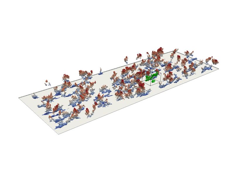
Fourth Madrid Summer School on Turbulence                                                                       IOP Publishing
Journal of Physics: Conference Series                         1522 (2020) 012009          doi:10.1088/1742-6596/1522/1/012009

Reynolds shear-stress carrying structures in
shear-dominated flows
                      Taygun R Gungor1,2 , Yvan Maciel2 , Ayse G Gungor1
                      1
                        Faculty of Aeronautics and Astronautics, Istanbul Technical University, 34469 Maslak,
                      Istanbul, Turkey
                      2
                        Department of Mechanical Engineering, Université Laval, Quebec City, QC, G1V 0A6
                      Canada
                      E-mail: taygun.gungor@itu.edu.tr

                      Abstract.
                          Four direct numerical simulation (DNS) databases are examined to understand the effect
                      of the wall and near-wall turbulence on the Reynolds shear-stress carrying structures in shear-
                      driven flows. The first DNS database is of a non-equilibrium adverse-pressure-gradient (APG)
                      turbulent boundary layer (TBL) with momentum thickness Reynolds number (Reθ ) reaching
                      8000. The second one is the same flow as the previous, but turbulence activity in the inner
                      layer (y/δ < 0.1) is artificially eliminated. The last two DNS databases are homogeneous shear
                      turbulence (HST) with Taylor microscale Reynolds numbers (Reλ ) are 104 and 248. Results
                      show that outer layer turbulence in the APG TBLs with large velocity defect is only slightly
                      affected by the near-wall region turbulence which suggests outer layer turbulence sustains itself
                      without necessitating near-wall turbulence. The Corrsin length scale (Lc ) scales the size of
                      the Reynolds shear-stress carrying structures in both APG TBLs and HSTs. The streamwise
                      length of these structures is 1Lc or larger in all cases. The aspect ratio of the structures behaves
                      similarly in both APG TBLs and HSTs when the size of the structures are normalized with Lc .
                      Sweeps and ejections tend to form side-by-side pairs in both flow types. The spatial properties
                      of sweeps and ejections, such as aspect ratios or relative positions are not affected by near-wall
                      turbulence activity or presence of the wall. This suggests that the structures mostly dependent
                      on the local mean strain rates.

1. Introduction
A turbulent boundary layer (TBL) subjected to an adverse pressure gradient (APG) develops
a large mean velocity defect. This velocity defect significantly alters the nature of the flow.
In canonical wall-bounded flows such as channel flows or zero-pressure-gradient (ZPG) TBLs,
turbulence activity is predominantly found in the near-wall region. In contrast, Reynolds stresses
peak in the outer layer in APG TBLs [1, 2] and turbulence production in the outer layer is much
higher in APG TBLs than in ZPG TBLs [3]. These findings which highlight an important
distinction between APG TBLs and canonical flows indicate the importance of outer layer in
the APG TBLs
   The intense uv structures, herein called Q structures, are streaky, streamwise elongated
and mostly concentrated in the near-wall region in ZPG TBLs and APG TBLs with small
velocity defect. [4]. In the outer layer, most of the Reynolds shear stress is carried by the wall-
attached (structures whose minimum wall-normal location is in the vicinity of the wall), tall

              Content from this work may be used under the terms of the Creative Commons Attribution 3.0 licence. Any further distribution
              of this work must maintain attribution to the author(s) and the title of the work, journal citation and DOI.
Published under licence by IOP Publishing Ltd                          1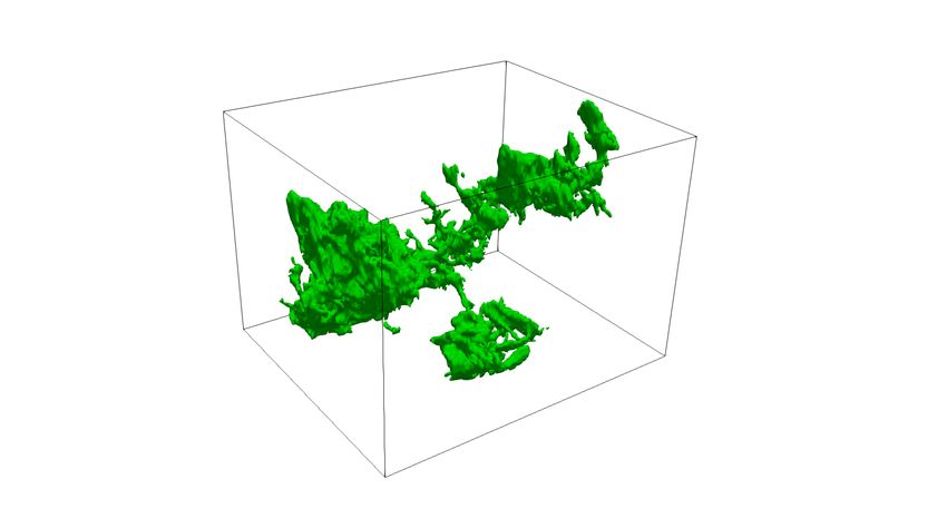
Fourth Madrid Summer School on Turbulence                                              IOP Publishing
Journal of Physics: Conference Series       1522 (2020) 012009   doi:10.1088/1742-6596/1522/1/012009

and streamwise elongated structures [4] as happens in the logarithmic and wake layer of channel
flows [5]. However, the situation in APG TBLs with large velocity defect considerably differs.
Consistent with the behavior of Reynolds stresses, Reynolds shear-stress carrying structures
(Q structures) are mostly found in the outer layer of APG TBLs. The near-wall Q structures
become disorganized and less numerous with increasing velocity defect [6]. Furthermore, the
structures found in the outer layer become stronger than their counterparts in the near-wall
region [4]. Even if both attached and detached structures are streamwise elongated, detached
structures are slightly more isotropic than attached structures in APG TBLs when the defect is
large [6].
   Gungor et al. [1] demonstrated that Reynolds stresses and turbulence kinetic energy budgets
behave similarly in the outer layer of APG TBLs and free shear layer flows such as mixing layer
flows. This similarity suggests that the wall does not significantly affect turbulence in APG
TBLs with a large velocity defect. The effect of the wall on shear flows was investigated by
Dong et al. [7]. They compared structures in channel flows and homogeneous shear turbulence
(HST) to distinguish the effect of wall and shear. They found that in both cases the Reynolds
shear stress is carried by Q structures that are larger than the Corrsin length scale, which is
defined as Lc = (/S 3 )1/2 where  is the turbulence dissipation and S is the mean shear. It
represents the scale of the smallest structures that interact directly with the mean shear. Below
Lc = 1, the turbulent structures become isotropic and decoupled from the mean shear. More
importantly, it was found that the spatial properties of the large Qs were similar in both types
of flows. The authors concluded that large Q structures are linked to local mean shear, rather
than to the presence of a wall.
   The present work aims to verify the latter conclusion in the case of APG TBLs with large
velocity defect and also to determine if outer-layer turbulence depends on near-wall turbulence
in these flows. To do so, we investigate the spatial properties of the Q structures in four DNS
databases that are the APG TBL of Gungor et al. [8], the same APG TBL but with inner
layer turbulence artificially eliminated, and two HST databases of Dong et al. [7] with Taylor
microscale Reynolds numbers (Reλ ) at 104 and 248.

2. DNS Databases
Four databases are used to investigate the Reynolds shear-stress carrying structures in shear
dominated flows. The first database (oAPG), described in Ref. [8], is a non-equilibrium APG
TBL subjected to a strong APG that leads to an increasing mean velocity deficit. The flow
evolves from a ZPG TBL to an APG TBL near separation. The DNS is performed with a
box domain over a no-slip smooth wall, with spanwise periodicity and streamwise non-periodic
inflow and outflow. The Reynolds number based on momentum thickness (Reθ ) spans between
1500-8200 and the shape factor (H) increases from 1.4 to 3.0.
    The second database (mAPG) is a non-equilibrium APG TBL, as well. The two APG TBLs,
oAPG and mAPG, are the same flow cases with a major difference. In mAPG, the turbulence
activity in the inner layer, which is defined as the region where the wall-distance (y) is below
0.1 of the local boundary layer thickness (δ), is artificially eliminated. The region where the
turbulence activity is eliminated starts at x ≈ 10δ0 , where δ0 is δ at the inlet. The height
of the region smoothly reaches y = 0.1δ in 10δ0 in the streamwise direction to prevent any
kind of numerical issues. The DNS code employs a spectral method in the periodic spanwise
direction [9, 10]. To eliminate the turbulence activity in the inner layer, all modes except the
zeroth mode are set to zero at every time step.
    The lack of turbulence in the inner region significantly affects the mean flow field. In order
to keep both cases identical, the spanwise- and time-averaged mean velocity profile from the
original APG TBL case is imposed to the zeroth mode of the modified APG case throughout
the boundary layer. Therefore, mean flow in both cases and hence integral variables such as δ ∗

                                                 2
Fourth Madrid Summer School on Turbulence IOP Publishing
Journal of Physics: Conference Series 1522 (2020) 012009 doi:10.1088/1742-6596/1522/1/012009
oAPG H = 2.5 y/δ = 1
a) H = 1.6
max(huui) in y
mAPG
b)
y/δ = 0.1
Figure 1. Streamwise velocity fluctuations (huui/Ue,0 2 ) of the APG TBLs as a function of
x/δ0 and y/δ0 . Top figure is the original APG TBL and the bottom figure is the manipulated
APG TBL. δ0 is δ at the inlet and Ue,0 is the velocity at the boundary layer edge at the inlet.
Straight and dashed black lines indicate the boundary layer edge and wall-normal location of
the maximum huui/Ue,0 2 , respectively. The dash-dotted line in (b) shows the interface between
the turbulent and non-turbulent region in the inner layer (y/δ = 0.1).
or θ and the total mass are identical. This database is generated to examine the effect of the
wall and inner layer turbulent activity on the Reynolds shear-stress carrying structures in the
outer layer of APG TBLs.
The other two databases are HST databases, which are described in detail in Ref. [11] and
[7]. The Reynolds numbers based on the Taylor microscale (Reλ ) of these databases are 104
(HST1) and 248 (HST2). They are chosen to investigate the effect of the wall and the mean
strain field on the outer layer coherent structures in APG TBLs.
3. Flow Description of the APG TBLs
In order to understand the effect of the near-wall region turbulent activity on the outer layer
turbulence, the turbulence statistics and Reynolds shear-stress budget of both APG TBLs are
compared. Figure 1 shows the streamwise evolution of huui of oAPG and mAPG as a function
of x/δ0 and y/δ0 . The boundary layer grows in height as the flow develops. The maximum
value of huui moves to the outer layer at approximately 28δ0 in oAPG. It is clearly seen that
the dominant turbulence energy is in the outer layer when the defect is large. The region where
turbulence is eliminated in mAPG is seen in figure 1b. The interface between the turbulent and
non-turbulent regions is at y/δ = 0.1. Besides the lack of turbulence in the inner layer, the
behavior of turbulence in the outer layer is very similar in both flows.
Figure 2 displays wall-normal profiles of huui and -huvi of oAPG and mAPG at two streamwise
positions corresponding to H = 1.6 and 2.5, as shown in figure 1, along with the ZPG TBL of
Sillero et al. at Reθ = 6000 [9]. Reynolds stresses are normalized with Zagarola-Smits velocity
(UZS = Ue δ ∗ /δ, where Ue is the velocity at the boundary layer edge and δ ∗ is the displacement
3Fourth Madrid Summer School on Turbulence IOP Publishing
Journal of Physics: Conference Series 1522 (2020) 012009 doi:10.1088/1742-6596/1522/1/012009
a) 0.5 b) 0.05
0.4 0.04
0.3 0.03
0.2 0.02
0.1 0.01
0 0
0 0.2 0.4 0.6 0.8 1 1.2 0 0.2 0.4 0.6 0.8 1 1.2
Figure 2. (a) and - (b) of oAPG and mAPG as a function of y/δ at two streamwise
positions corresponding to small (H = 1.6) and large (H = 2.5) velocity defect situations along
with the ZPG TBL of Sillero et al. [9]. Blue, red and green straight lines indicate the large and
small velocity regions of the original APG TBLs and the ZPG TBL, respectively. The blue and
red dashed lines indicate the large and small velocity defect regions of the manipulated APG
TBL, respectively. Turbulence statistics are normalized with UZS .
thickness). The original APG TBL (solid lines) behaves almost like a ZPG TBL when the
velocity defect is small (H = 1.6). Near-wall turbulence activity is less intense but the well-
known inner peak of huui is present. All Reynolds stresses decrease with increasing velocity
defect when they are normalized with UZS . Furthermore, turbulence activity in the inner
region reduces considerably and the outer layer turbulence becomes dominant. This behavior
of turbulence with increasing velocity defect demonstrates the importance of the outer layer in
APG TBLs and highlights the main distinction between APG and ZPG TBLs [1, 2].
The turbulence statistics of mAPG, shown in figure 2 with dashed lines, present that
turbulence has effectively been removed in the inner region, y/δ = 0.1. Above y/δ = 0.1,
there is an immediate increase in both and -. This sharp increase is similar to the
behavior of turbulence in the region just above the wall in wall-bounded flows. For the small
velocity-defect position at H = 1.6, both Reynolds stresses of mAPG recover values comparable
to those of oAPG at approximately y/δ = 0.45. There is almost a perfect match for both cases
above that point. However, this is not the case for the large velocity-defect position at H = 2.5,
where the Reynolds stresses of mAPG remain slightly smaller than those of oAPG. Despite the
differences, the results suggest that turbulence in the outer layer can sustain itself in the absence
of near-wall turbulent activity.
Figure 3 presents the Reynolds shear stress budget of oAPG and mAPG as a function of y/δ
for the two streamwise positions. The Reynolds shear-stress budget is given as follows.
D̄hui uj i ∂hui uj uk i 2 hUj i hUi i 1 ∂p ∂p ∂ui ∂uj
=- + ν∇ hui uj i- hui uk i + huj uk i - hui + uj i-2νh i (1)
D̄t ∂xk ∂xk ∂xk ρ ∂xj ∂xi ∂xk ∂xk
Here ν is viscosity, U and u indicate the instantaneous and fluctuating velocity and h.i is
the averaged values. The terms are, in order, mean convection, turbulence convection, viscous
diffusion, production, pressure and dissipation. Near the interface between the non-turbulent
and turbulent regions in mAPG, there is a nonphysical behavior due to the transition from
the non-turbulent region to the turbulent region. It is important to state that this kind of
nonphysical behavior near the interface is excepted. Despite this nonphysical behavior, the
4Fourth Madrid Summer School on Turbulence IOP Publishing
Journal of Physics: Conference Series 1522 (2020) 012009 doi:10.1088/1742-6596/1522/1/012009
a) 0.4 b)
0.1
0.2
0.05
0 0
-0.05
-0.2
H=1.6 -0.1
H=2.5
-0.4
0 0.2 0.4 0.6 0.8 1 1.2 0 0.2 0.4 0.6 0.8 1 1.2
Figure 3. The budget of -huvi oAPG and mAPG as a function of y/δ at two streamwise
positions corresponding to H = 1.6 and H = 2.5. Straight and dashed lines indicate oAPG and
mAPG respectively. Red, blue, magenta, black and green lines indicate production, dissipation,
turbulent convection, mean convection, and pressure terms, respectively. The budget terms are
normalized with UZS and δ.
contribution of different terms to the -huvi balance follow the same trend. Whereas the values
of the budget of oAPG and mAPG are almost exactly the same in the region where y/δ above
0.3 of the small defect position, there is a difference between oAPG and mAPG in the large
defect position.
As previously mentioned, the outer layer turbulence is dominant and much more important
than the inner layer turbulence activity in APG TBLs with large velocity defect. That the
turbulence production peaks in the outer layer supports this, as well. APG TBLs with large
velocity defect have similarities with free shear layer and mixing layer flows [1]. Hence the
following section scrutinizes this similarity between HSTs and APG TBLs.
4. Similarities of Shear Dominated Flows
The Corrsin shear parameter defined as S ∗ = Sq 2 /, where S is the mean shear, q 2 is twice of the
turbulence kinetic energy and is the turbulence dissipation, is the ratio of turbulence dissipation
time to the mean shear deformation time. It measures the importance of the interaction of the
shear with the energy-containing eddies. When S ∗ >> 1, the flow and the turbulence scales are
dominated by the mean shear, and when S ∗ . O(1) turbulence is decoupled from the mean shear
[12]. Figure 4(a) presents S ∗ as a function of y/δ for two streamwise positions of oAPG and
mAPG corresponding to H = 1.6 and 2.5 and the ZPG TBL database of Ref [9] at Reθ = 6000.
Below y/δ = 0.3, in the near-wall region, S ∗ is very high but it suddenly drops, then slowly
increases. Above y/δ = 0.8, S ∗ slowly tends to zero, which indicates that the effect of the mean
shear diminishes in this region. Between y/δ = 0.3 − 0.8, S ∗ is almost constant for all cases and
approximately 10. That S ∗ is almost constant and S ∗ >> 1 between y/δ = 0.3 − 0.8 implies
that the mean shear dominates the large-scale turbulent structures in the outer region of the
boundary layers. S ∗ in HSTs is approximately 7.5 [7]. The values of S ∗ in APG TBLs and HSTs
are similar.
In order to understand these similarities between two APG TBLs and shear-driven flows,
the premultiplied cospectra of the two APG TBLs and HSTs are examined. Figure 4(b) shows
the premultiplied 1D co-spectra of the large defect position at H = 2.5 of oAPG and mAPG
at y/δ = 0.5 along with the co-spectra of HSTs as a function of the streamwise wavelength
5Fourth Madrid Summer School on Turbulence IOP Publishing
Journal of Physics: Conference Series 1522 (2020) 012009 doi:10.1088/1742-6596/1522/1/012009
a) 25 b) 0.4
20
0.3
15
0.2
10
0.1
5
0
0
0 0.2 0.4 0.6 0.8 1 10 -2 10 -1 10 0 10 1 10 2
Figure 4. (a) Corrsin shear parameter, S ∗ , of two streamwise locations of oAPG and mAPG
corresponding to H = 1.6 and H = 2.5 and ZPG TBL as a function of y/δ. The vertical lines
indicate the region between y/δ = 0.3 and 0.8 where S ∗ is almost constant. (b) Premultiplied
1D co-spectra of the APG TBLs at y/δ = 0.5 and HSTs as a function of λx /Lc . Blue, red, green
and black indicate oAPG, mAPG, HST1 and HST2, respectively.
(λx ). The spectra of the APG TBLs are obtained using temporal data. The temporal data is
transformed into spatial data by employing Taylor’s frozen turbulence hypothesis based on the
local mean velocity. The spectra are normalized with the friction velocity (uτ ). Since the wall
does not exist in the case of HST, uτ is defined as u2τ = νS −h|uv|i [7]. The same definition of the
friction velocity is employed for the APG TBLs. λx is normalized with Lc . The premultiplied
co-spectra from both APG TBLs matches very well. The co-spectra of HSTs and the APG
TBLs have similar trends, but λx /Lc of the peak of the co-spectra differ from each other. While
the peak of the HSTs is at approximately 15Lc , peaks of APG TBLs are at approximately
10Lc . Even though the co-spectra of the cases are slightly different from each other, Lc appears
to be a suitable characteristic length scale for the Reynolds shear-stress carrying structures in
shear-dominated flows.
5. Spatial properties of the Reynolds shear-stress carrying structures
5.1. Structure Identification Method
Q structures are identified to investigate the spatial properties of Reynolds shear-stress carrying
structures. They are divided into four based on their quadrant positions in the u-v plane:
outward interactions (Q1, u > 0 and v > 0), ejections (Q2, u < 0 and v > 0), inward interactions
(Q3, u < 0 and v < 0) and sweeps (Q4, u > 0 and v < 0). The present study focuses on Q2 and
Q4 events. Q structures are defined as connected regions satisfying the following condition [5]
u(x)v(x)| > H ∗ σu σv , (2)
where H ∗ is the threshold constant which is also called hyperbolic-hole size and σ is the root-
mean-square. Connectivity is defined with the six orthogonal neighbors in the mesh of the
DNS. For this study, a percolation analysis is not performed. H ∗ = 1.75 is chosen based on the
previous channel flow study of Lozano et al. [5] and the APG TBL study of Maciel et al. [6].
This technique has been used for channel flows [5], APG and ZPG TBLs [6, 13] and
homogeneous shear turbulence [7] using spatial data. In the current study, the Q structures of
the APG TBLs are detected using temporal data collected at every time step at one streamwise
location corresponding to large defect position (H = 2.5) from the whole y − z plane. The
6Fourth Madrid Summer School on Turbulence IOP Publishing
Journal of Physics: Conference Series 1522 (2020) 012009 doi:10.1088/1742-6596/1522/1/012009
a)
0
6
∆z
6 12
tUZS /δ ∆y
b)
z/δ
18
0
∆x
Figure 5. (a) Spatio-temporal evolution of Q2 structures at H = 2.5. The temporal data are
transformed into spatial data using local UZS and δ. The structures are colored by the distance
to the wall, from y/δ = 0 for the blue to y/δ = 1.2 for the red. (b) Perspective view of a Q2
structure with the circumscribing box. The dimensions of the box are denoted ∆x, ∆y and ∆z
corresponding to streamwise, wall-normal and spanwise directions, respectively.
temporal data is converted into spatial data using Taylor’s frozen turbulence hypothesis. The
local mean velocity at the center of the structure is assumed to be its convective velocity. The
center of the structures is calculated as the arithmetic mean of the maximum and minimum y
locations of the structures. For HST, spatial data are employed to identify the Q structures. As
it was mentioned before, S ∗ is almost constant between y/δ = 0.3 − 0.8 for both APG TBLs.
Therefore, only the structures whose centers are in this region are considered in the analysis. In
addition to this, wall-attached structures, defined with a minimum wall distance of 0.05y/δ or
lower, are discarded, as well, because shape and orientation of the wall-attached structures are
significantly different from those of the wall-detached structures [7]. Furthermore, very small
Q structures that have a volume smaller than 3(∆z)3 are rejected, because their size is too
small for the numerical grid. Figure 5 displays the spatio-temporal development of the 3D Q2
structures obtained using the structure detection method and a single Q2 structure with the
circumscribing box. The dimensions of the box are employed to define and analyze the spatial
properties of the structures.
5.2. Aspect Ratios of the Q2 and Q4 Structures
The shape and orientation of the structures can be investigated through their aspect
ratios. Figure 6 presents joint probability density functions (pdfs) of dimensions of the box
circumscribing the wall-detached Q2 and Q4 structures in the region of interest for oAPG and
mAPG. When the streamwise and spanwise dimensions of the boxes are less than approximately
0.5δ, the structures are mostly isotropic. As the streamwise size of the structures increases,
the structures become streamwise elongated. Furthermore, Q2 structures are slightly more
streamwise oriented than Q4 structures. Although there are minor differences between the
structures in oAPG and mAPG, the spatial properties of the structures in both APG TBLs are
very similar to each other. Joint pdfs of ∆x and ∆y, and ∆z and ∆y of the structures in oAPG
and mAPG are also consistent with the study of Maciel et al. [4] that was performed using
the spatial data. They reported that detached Q2 and Q4 structures are slightly streamwise
elongated in ZPG and APG TBLs, too.
7Fourth Madrid Summer School on Turbulence IOP Publishing
Journal of Physics: Conference Series 1522 (2020) 012009 doi:10.1088/1742-6596/1522/1/012009
10 1 10 1
10 0 10 0
10 -1 10 -1
10 -2 10 -2
10 -2 10 -1 10 0 10 1 10 -2 10 -1 10 0 10 1
10 1 10 1
10 0 10 0
10 -1 10 -1
10 -2 10 -2
10 -2 10 -1 10 0 10 1 10 -2 10 -1 10 0 10 1
---------------------------------------------–-------------------
10 1 10 1
10 0 10 0
10 -1 10 -1
10 -2 10 -2
10 -2 10 -1 10 0 10 1 10 -2 10 -1 10 0 10 1
10 1 10 1
10 0 10 0
10 -1 10 -1
10 -2 10 -2
10 -2 10 -1 10 0 10 1 10 -2 10 -1 10 0 10 1
Figure 6. Joint pdf of ∆y /δ and ∆x /δ (left column), and ∆y /δ and ∆z /δ (right column) for
Q2 and Q4 structures. From top to bottom, Q2 of oAPG, Q2 of mAPG, Q4 of oAPG and
Q4 of mAPG. Contours levels are [0.06:0.4:3.64]. Axes are normalized with δ. The dashed line
indicates ∆x /δ = ∆y /δ and ∆z /δ = ∆y /δ. 8Fourth Madrid Summer School on Turbulence IOP Publishing
Journal of Physics: Conference Series 1522 (2020) 012009 doi:10.1088/1742-6596/1522/1/012009
1.5
1
4
2
0.5
100 101 102
10 0 10 1
Figure 7. Average aspect ratio of the circumscribing boxes for combined Q2 and Q4 structures
as a function of the box diagonal (d) of the structure. The box diagonal is normalized with Lc .
Blue, red, green and black lines indicate oAPG, mAPG, HST1 and HST2. Filled (-N- and --)
and empty (-◦- and --) symbols indicate ratio of ∆x to ∆y (axy ) and ratio of ∆z to ∆y (azy ),
respectively. The figure in the inset is the same figure with larger axis ranges.
Figure 7 presents the average aspect ratio (aij , the ratio of ∆i to ∆j) of the circumscribing
boxes for Q2 and Q4 structures in oAPG, mAPG and HSTs as a function of the diagonal of
the boxes (d). The box diagonal is normalized with Lc . The aspect ratios in both APG TBLs
perfectly match regardless of the box diagonal. This shows that the inner layer turbulence
activity does not change the shape of the Reynolds shear-stress carrying structures in the outer
layer. In both APG TBLs and HSTs, there is a similar trend: azy steadily decreases between
d/Lc = 1 − 10 from values above one to about 0.8. In the APG TBLs, azy increases after
d/Lc = 10, but in HSTs it continues to decrease. axy of HSTs very slightly increases until
diagonal of the boxes becomes approximately 30LC . axy is always above one for all flows, but
the streamwise elongation is small except for very large Q structures in the APG TBLs. axy
of the APG TBLs remains fairly constant for small structures but it dramatically increases
after d/Lc = 10. The reason of this dramatic increase in axy and weak increase in azy is
probably that the structures are bounded in the wall-normal direction and unbounded in the
streamwise direction. As the structures become larger, they cannot grow in the wall-normal
direction because of the presence of the wall. In HST, the flow is unbounded in the wall-normal
direction, so they keep growing in that direction as well [7]. The detached Q structures with
diagonal smaller than approximately 3Lc in channel flows are mostly isotropic, however their
axy is slightly larger than axy of the structures in HSTs [7].
For azy , there is a perfect match for all the cases when d/Lc is between 1 − 10. Although axy
of the APG TBLs and HSTs behave slightly differently from each other, the values of axy of the
four cases are very close. Overall, in both HSTs and APG TBLs, the structures become more
streamwise elongated and narrower in the spanwise direction as the structures become larger.
The Reynolds shear-stress carrying structures have therefore similar geometrical features in both
types of flows. The situation for channel flows is also similar to HSTs and APG TBLs [7].
5.3. Relative positions of Q2 and Q4 Structures
Spatial organization of Q structures is analyzed through relative positions of Q structures.
Figure 8 presents the joint pdfs, pij (rx , rz ), of relative positions of Q structures of the same and
different kind in oAPG and mAPG in a wall-parallel plane. Indices i and j stand for quadrant
9Fourth Madrid Summer School on Turbulence IOP Publishing
Journal of Physics: Conference Series 1522 (2020) 012009 doi:10.1088/1742-6596/1522/1/012009
2 0.5 2 2
1 1
1 1
1 1 1.5 1.5 1.5
1.5 1.5
1.5 2
1 2
1 2.5 1 2 2
2 2
2.5 2.5 3.5
3
3
3
2.5
2.5
2.5
3
4
3 2.5 2
4 2 2 2
0 3.5 0 1.5 0 1.5 1
3.
0.5 1 1.5 0.5
5
3.5 3.5 3
1.5
3 2.5
2.5 1.
5
2
2
1
-1 -1 -1
1
1.5 1.5 1
1 1
1 1
0.5 0.5 0.5 0.5 0.5
-2 -2 -2
-2 -1 0 1 2 -2 -1 0 1 2 -2 -1 0 1 2
2 2 2
1 1 1 1
1
1 1.5
1.5 1.5 1.5
1.5
1.5 2 2
1 1 2 2.5 1 2
2 2 2.5
3
2.5 3
2.5 2.5
3.5 2
2.5
3 3 3.54 2.5 3 2
4 2 2
5
0 0 1.5 0 1.5
3.
1.5 1
3 3 0.5 0.5
1
1.5
2.5 2.5
2 1
1.5
2
-1 1.5 -1 -1
1
1.5
1 1 1
1 1
1
0.5 0.5 0.5
-2 -2 -2
-2 -1 0 1 2 -2 -1 0 1 2 -2 -1 0 1 2
Figure 8. Joint pdfs of relative positions of Q2 structures with respect to Q2 structures, p22
(left), Q4 structures with respect to Q2 structures p42 (center), Q2 structures with respect to Q4
structures p24 (right). Top row is oAPG and the bottom row is mAPG. Contours are normalized
with the probability at long distance (pf ar ).
of Q structures. The relative positions of i structure with respect to j structure are obtained as,
xj − xi zj − zi
rx = and rz = , (3)
0.5(dj + di ) 0.5(dj + di )
p
where di = ∆xi2 + ∆z i2 is the wall-parallel diagonal length of the structure and, x and z are
the spatial coordinates of the structures. The temporal data is employed to obtain the relative
positions of Q structures. A single convection velocity (mean velocity at y/δ = 0.5) is used to
transform the temporal data into spatial data. In order to reduce the effect of using a single
convection velocity for all structures, only the structures between y/δ = 0.4 − 0.7 are considered
for this analysis.
Q2 structures of the same kind tend to form an upstream-downstream configuration in both
APG TBLs. This is also true for the relative positions of Q4 structures with respect to Q4
structures, although it is not presented here. The pdfs of relative positions of Q structures
of different kind are intentionally weighted towards positive rz to test the symmetry of the
structures in the spanwise direction. The weighting is performed by choosing the direction of
nearest Q structure of different kind as a positive direction (rz > 0). This means that a secondary
peak with negative rz , in addition to the primary one with rz > 0, indicates the presence of
Q structures surrounded by two Q structures of the other type. Conversely, a weak secondary
peak points to presence of side-by-side sweeps and ejections pairs. Side-by-side pairs are indeed
the most dominant configuration in both APG TBLs. The results in both APG TBLs are very
10Fourth Madrid Summer School on Turbulence IOP Publishing
Journal of Physics: Conference Series 1522 (2020) 012009 doi:10.1088/1742-6596/1522/1/012009
similar to each other, suggesting that near-wall turbulence activity does not affect the spatial
organization of outer Q structures. The pdfs of relative positions of Q structures in oAPG
and mAPG are also consistent with the paper of Maciel et al. [4]. They found that streamwise
alignment of Q structures of the same kind and presence of side-by-side sweeps and ejections are
the most probable events in APG and ZPG flows. Furthermore, similar results were reported
for the outer layer of channel flows by Lozano et al. [5] and HSTs by Dong et al. [7].
6. Conclusion
In this study, APG TBL and HST DNS databases are analyzed to investigate the Reynolds shear-
stress carrying structures in shear-dominated flows. These databases are chosen to understand
the effect of the inner layer turbulent activity and the wall on the outer layer Reynolds shear-
stress carrying structures in APG TBLs. Turbulence statistics of the two APG TBL cases
indicate that the elimination of turbulence in the inner layer only slightly reduces outer layer
turbulence. Furthermore, Reynolds shear-stress carrying structures in the outer layer of both
APG TBLs have almost identical spatial properties. Outer layer turbulence is therefore not
significantly affected by inner layer turbulence. Moreover, detached Q2 and Q4 motions in both
APG TBLs and HSTs have very similar geometric properties for the structures whose diagonal
length, d, is less than approximately 8Lc . Furthermore, structures in channel flows behave
similarly until d becomes approximately 3Lc . The relative positions of Q2 and Q4 structures in
all these flows are very similar too. All these results indicate that the wall and the near-wall
turbulence activity do not heavily affect the spatial properties of outer Reynolds shear-stress
carrying structures in TBLs. These structures appear to be mostly dependent on the local mean
strain rates.
7. Acknowledgments
The authors would like to thank Prof. Javier Jiménez for organizing the Fourth Madrid
Turbulence Workshop. The computational resources were provided by Calcul Québec
(www.calculquebec.ca) and Compute Canada (www.computecanada.ca). This work was also
funded in part by the Coturb program of the European Research Council, Istanbul Technical
University BAP Unit (Project number MDK-2018-41689) and NSERC of Canada. The authors
would like to thank Siwei Dong, Adrián Lozano-Durán, Atsushi Sekimoto and Prof. Javier
Jiménez for providing their HST data, and to Prof. Julio Soria for carefully reviewing the
original manuscript.
References
[1] A. G. Gungor, Y. Maciel, M. P. Simens, and J. Soria. Scaling and statistics of large-defect adverse pressure
gradient turbulent boundary layers. Int. J. Heat Fluid Flow, 59:109–124, 2016.
[2] Y. Maciel, T. Wei, A. G. Gungor, and M. P. Simens. Outer scales and parameters of adverse-pressure-gradient
turbulent boundary layers. J. Fluid Mech., 844:5–35, 2018.
[3] P. E. Skåre and P. Krogstad. A turbulent equilibrium boundary layer near separation. J. Fluid Mech.,
272:319–348, 1994.
[4] Y Maciel, A G Gungor, and M P Simens. Structural differences between small and large momentum-defect
turbulent boundary layers. Int. J. Heat Fluid Flow, 67:95–110, 2017.
[5] A. Lozano-Durán, O. Flores, and J. Jiménez. The three-dimensional structure of momentum transfer in
turbulent channels. J. Fluid Mech., 694:100–130, 2012.
[6] Y. Maciel, M. P. Simens, and A. G. Gungor. Coherent structures in a non-equilibrium large-velocity-defect
turbulent boundary layer. Flow Turbul. Combust., 98:1–20, 2017.
[7] S. Dong, A. Lozano-Durán, A. Sekimoto, and J. Jiménez. Coherent structures in statistically stationary
homogeneous shear turbulence. J. Fluid Mech., 816:167–208, 2017.
[8] A. G. Gungor, Y. Maciel, M. P. Simens, and T. R. Gungor. Direct numerical simulation of a non-equilibrium
adverse pressure gradient boundary layer up to Reθ = 8000. In 16th Europ. Turbul. Conf., Stockholm,
Sweden, Europ. Mechanics Soc., 2017.
11Fourth Madrid Summer School on Turbulence IOP Publishing
Journal of Physics: Conference Series 1522 (2020) 012009 doi:10.1088/1742-6596/1522/1/012009
[9] J. A. Sillero, J. Jiménez, and R. D. Moser. One-point statistics for turbulent wall-bounded flows at Reynolds
numbers up to δ + ≈ 2000. Phys. Fluids, 25:105102, 2013.
[10] G. Borrell, J. A. Sillero, and J. Jiménez. A code for direct numerical simulation of turbulent boundary layers
at high Reynolds numbers in BG/P supercomputers. Comput. Fluids, 80:37–43, 2013.
[11] A. Sekimoto, S. Dong, and J. Jiménez. Direct numerical simulation of statistically stationary and
homogeneous shear turbulence and its relation to other shear flows. Phys. Fluids, 28:035101, 2016.
[12] J. Jiménez. Near-wall turbulence. Phys. Fluids, 25:101302, 2013.
[13] C. Atkinson, A. Sekimoto, J. Jiménez, and J. Soria. Reynolds stress structures in a self-similar adverse
pressure gradient turbulent boundary layer at the verge of separation. In J. of Physics: Conf. Ser.,
volume 1001, page 012001. IOP Publishing, 2018.
12You can also read