Spatial ecology and habitat partitioning of two sympatric ophichthid eel species in the Gulf of Mexico
←
→
Page content transcription
If your browser does not render page correctly, please read the page content below
Bull Mar Sci. 99(2):71–94. 2023
                                                                                  research paper
https://doi.org/10.5343/bms.2022.0031

Spatial ecology and habitat partitioning of two
sympatric ophichthid eel species in the Gulf of Mexico

1
 College of Marine Science,                        Steven A Murawski 1 *
University of South Florida,
                                                   Adolfo Gracia 2
140 7th Avenue South, St.
Petersburg, Florida 33706
2
 Instituto de Ciencias del Mar
y Limnología, Universidad
Nacional Autónoma de                                  ABSTRACT.—Ophichthid eel species are abundant and
México, Apartado Postal                            diverse in tropical and semitropical seas but there are few
70-305, Mexico City, 04510,
                                                   studies of snake eel life histories and factors influencing
Mexico
                                                   spatial distributions. Here we analyze 12 demersal longline
* Corresponding author email:                      sampling expeditions circumnavigating continental
                                shelves in the Gulf of Mexico (GoM) during 2011–2017.
                                                   Two ophichthid eels were dominant components of fish
                                                   assemblages: king snake eel (KSE), Ophichthus rex, and
                                                   palespotted eel (PSE), Ophichthus puncticeps. Relative
                                                   abundance (CPUE) of KSE was highest in the north central
                                                   GoM, lower in the northwest and southeast and on the West
                                                   Florida Shelf, and absent from northwest Cuba and the
                                                   Yucatán Platform. Contrariwise, PSE abundance was highest
                                                   on the Yucatán Platform, lower in the north central GoM and
                                                   on the West Florida Shelf, and absent from the northwest and
                                                   southwest GoM and Cuba. GAM-based species distribution
                                                   models were fit to presence-absence data from sampled
                                                   stations using a variety of environmental covariates including
                                                   water depth, longitude, and sediment type (sand vs mud/silt).
                                                   Although the two species were caught in similar depths and
                                                   bottom temperatures, they were only caught together at 1%
                                                   of the stations. This study extends the record length of KSE
                                                   to 226 cm (total length). Despite being abundant in areas
                                                   overlapping the footprint of the Deepwater Horizon oil spill
                                                   in 2010, concentrations of polycyclic aromatic hydrocarbons
                                                   (PAHs) and their metabolites were relatively low in KSE,
                                                   perhaps related to copious slime production which, in other
                                                   studies, has been determined to be a vector for PAH excretion
                                                   in fishes.

                                                      RESUMEN.—Las especies de anguilas ofictidas son
                                                   abundantes y diversas en los mares tropicales y semitropicales;
                                                   sin embargo existen pocos estudios sobre las historias de
                                                   vida de las anguilas serpiente y los factores que influyen en
                                                   sus distribuciones espaciales. En este estudio analizamos
                                                   12 expediciones de muestreo con palangre demersal
                                                   desarrolladas en la plataforma continental de todo el Golfo de
Date Submitted: 25 August, 2022.                   México (GoM) durante 2011–2017. Dos anguilas Ophichthid
Date Accepted: 9 February, 2023.
Available Online: 10 February, 2023.               fueron componentes dominantes en los conjuntos de peces:

Bulletin of Marine Science                                           71
© 2023 Rosenstiel School of Marine, Atmospheric & Earth Science of
the University of Miami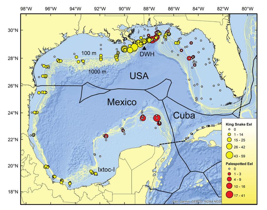
72                       Bulletin of Marine Science. Vol 99, No 2. 2023

                              lairón (KSE), Ophichthus rex, y tieso de puntos pálidos (PSE),
                              Ophichthus puncticeps. La abundancia relativa (CPUE) de
                              KSE fue más alta en el centro norte del GoM, menor en el
                              noroeste y suroeste y en la plataforma del oeste de Florida, y
                              nula en el noroeste de Cuba y la plataforma de Yucatán. Por el
                              contrario, la abundancia de PSE fue mayor en la plataforma de
                              Yucatán, menor en el centro norte del GoM y en la plataforma
                              occidental de Florida, y nula en el noroeste y suroeste del GoM
                              y en Cuba. Los modelos de distribución de especies basados
                              en GAM se ajustaron a los datos de presencia-ausencia
                              de las estaciones muestreadas utilizando una variedad de
                              covariables ambientales que incluyen la profundidad del agua,
                              la longitud, y el tipo de sedimento (arena frente a lodo/limo).
                              Aunque las dos especies se registraron en profundidades y
                              temperaturas de fondo similares, solo fueron capturadas
                              juntas en 1% de las estaciones. Este estudio extiende la
                              longitud máxima registrada de KSE a 226 cm (longitud total).
                              A pesar de ser abundante en áreas que contienen la huella
                              del derrame de petróleo de Deepwater Horizon en 2010, las
                              concentraciones de hidrocarburos aromáticos policíclicos
                              (HAP) y sus metabolitos fueron relativamente bajas en KSE,
                              tal vez relacionado con la producción copiosa de mucosidad
                              que, en otros estudios, se ha determinado como un vector
                              para la excreción de PAH en los peces.

   Eels of the family Ophichthidae (snake/worm eels, order Anguilliformes) represent
a diverse and speciose group distributed widely throughout tropical and warm tem-
perate oceans. The Ophichthidae contains the most genera and species of any anguil-
liform family, currently numbering 62 of 156 known genera and 359 of 1023 known
eel species (Fricke et al. 2023). The Gulf of Mexico (GoM) is inhabited by at least 44
ophichthid taxa (the union of lists compiled by McEachran and Fechhelm 1998 and
Moore et al. 2020), adjacent waters of the Florida Straits and southern Sargasso Sea
by at least 22 (Miller and McCleave 2007), the south- and mid-Atlantic continental
shelves off the USA by 38 species (Fahay and Obenchain 1978), and 30 species are
documented off North Carolina (Ross et al. 2006). They are found in diverse habitats,
from coastal areas to depths >1300 m. Most species are bottom dwellers, purportedly
burrowing into mud or sandy sediments where they ambush potential invertebrate
(primarily crustacean) and fish prey, although some primarily pelagic species ex-
ist. Despite their ubiquity and species richness, little is known about the life histo-
ries of the Ophichthidae primarily because of their cryptic habits as adults and the
lack of directed commercial or recreational fisheries for them. Routine trawl- and
camera-based surveys in the GoM do not index these species because of the low
catchability of these sampling gears to benthic juveniles and adults of ophichthid
eel species. In fact, most published information concerning the family is as a result
of scientific midwater trawling or plankton netting resulting primarily in catches of
their leptocephalus larvae (e.g., Fahay and Obenchain 1978, Ross et al. 2006, Miller
and McCleave 2007, Able et al. 2011, Collins 2019, Quattrini et al. 2019, Moore et
al. 2020) or from studies of some species as juveniles when they migrate to coastal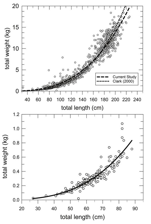
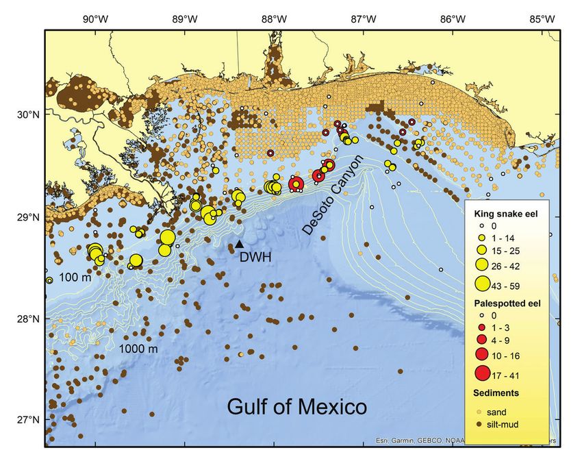
Murawski and Gracia: Spatial ecology of eels in the Gulf of Mexico      73

Figure 1. Geography of the Gulf of Mexico including isobaths from 100 to 1000 m (in 100 m
increments). Subregions are designated by dashed lines (consistent with Murawski et al. 2018).
Black heavy lines are the international territorial boundaries of countries in the region.

waters (Able et al. 2011). While some ophichthid eels are purported to form burrows,
there is little visual or experimental evidence to support general conclusions of habi-
tat use owing to the great depths and murky waters in which many species live. Given
the myriad of anthropogenically-based challenges to biodiversity in the GoM (e.g.,
fishing, oil and gas development, climate change, marine and coastal modifications,
pollution events, etc.) it is imperative that we better understand the life histories of
potentially at-risk species, particularly those with important functional roles in the
ecosystem.
   During 2011–2017 we conducted comprehensive longline-based surveys of the
continental shelves of the GoM (Murawski et al. 2018). The objectives of these sur-
veys, comprising 12 separate expeditions, were to evaluate oil-related pollution in
GoM fishes and potential impacts to species, particularly focusing on effects from
the Deepwater Horizon (DWH) oil spill that occurred in 2010 (Murawski et al. 2014,
2021, Snyder et al. 2015, Pulster et al. 2020). Single surveys were conducted off Cuba,
Mexico, Texas, and the western Louisiana coast to provide baselines from areas pre-
sumably not affected by DWH. A time series of surveys was conducted in the north
central Gulf, near the DWH site, to evaluate changes in pollutant body burdens, rela-
tive abundance, population demography, and disease status of species (Figs. 1 and 2).
Two ophichthid species king snake eel (KSE, aka Lairón in Mexico), Ophichthus rex,
and palespotted eel (PSE, aka Tieso de Puntos Pálidos in Mexico), Ophichthus punc-
ticeps—both in subfamily Ophichthinae (snake eels)—were the third and 15th most
74                          Bulletin of Marine Science. Vol 99, No 2. 2023

Figure 2. Numbers of king snake eels and palespotted eels captured at each longline fishing site
sampled in the Gulf of Mexico, 2011–2017. Locations of the 2010 Deepwater Horizon and the
1979–1980 Ixtoc 1 oil spill areas indicated by black triangles.

abundant species, respectively, taken in these longline surveys, resulting in a sub-
stantial data set of relative abundance, population demography, and distributional
determinants of their populations (Murawski et al. 2018).
   Here we analyze information obtained from these longline surveys to character-
ize the abundance, distribution, and population biology of both species. Using sur-
vey catches and associated environmental predictors we fit a hierarchical series of
species distribution models using generalized additive models (GAMs; Hastie and
Tibshirani 1986, 1990, Wood 2017) that allow a combination of nonlinear smooth-
ers and categorical variables to predict species presence/absence at specific locations
(e.g., Perryman and Babcock 2017). We also consider joint species distribution models
(JSDMs; Guisan and Thuiller 2005, Zurell et al. 2018, Poggiato et al. 2021, Wilkinson
et al. 2021) to examine the probability of co-occurrence of KSE and PSE. Results are
used to evaluate the significance of environmental factors determining species dis-
tributions and their implications in the face of long-term ecosystem change.

                                           Methods

  Field Sampling.—Longline sampling and related fish handling methods for the
surveys generating data analyzed herein are discussed in detail in Murawski et al.
(2018). Briefly, transects were sampled with nominal station placement in continen-
tal shelf waters from 40 to about 300 m deep. We used longline sampling (baited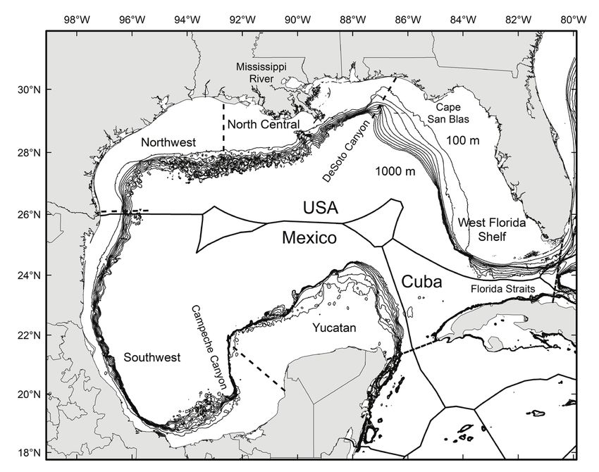
Murawski and Gracia: Spatial ecology of eels in the Gulf of Mexico   75

hooks) as standardized sampling methodology primarily to target large juvenile and
adult fishes occupying relatively high trophic levels and because the gear can be de-
ployed in bottom habitats where trawls and other bottom-tending mobile gears are
not appropriate.
   Longline sets were usually made at six stations along predefined transects that
extended from shallow to deep shelf regions (Fig. 2). Target sampling depths along
each transect were 37, 73, 110, 146, 183, and 274 m. In deeper areas the bathymetric
slope was so steep that six unique stations could not be effectively sampled and, in
some areas, depth control (fishing along an isobath) of those stations was difficult
(especially off NW Cuba and the western Yucatán Peninsula; Fig. 1). Thus, for some
stations, the average depth exceeded the nominal set depth, accounting for a few
outliers in the depth distributions of the two eel species.
   We chartered three commercial fishing vessels (2011–2012) and used the R/V
Weatherbird II (2012–2017) to deploy longline sets. At each station, 8 km (5 nm)
of 3.2 mm galvanized steel (2011–2012) or 544 kg test monofilament (2013–2017)
main line was deployed, with a mean of 446 baited hooks fished per set. We used
136 kg test leaders, 2.4 m long, clipped to the main line and attached to #13/0 circle
hooks. Bait was cut fish (Atlantic mackerel, Scomber scombrus) and squid (primarily
Humboldt squid, Dosidicus gigas, wings) which were deployed randomly during the
hook baiting process. At the beginning and end of each set, we deployed a “high-
flyer” buoy and attached Star:Oddi® CDST Centi temperature/time/depth (TTD)
recorders to the main line with sufficient scope to reach the bottom and to record
bottom time, bottom temperature (°C) and fished depth (m) at five min intervals.
At set-out and haul-back we recorded latitude and longitude, time, and depth (from
ships’ echosounders). Fishing occurred only during daylight hours. Average soak
time of sets was 2.08 hrs.
   At retrieval, we determined species and recorded the total length (cm) of each
eel caught. Each specimen was weighted to the nearest g on a Marel® motion-
compensated scale, or hand scale (nearest 0.1 kg) for large fish (>6 kg). For a subset
of the KSE catch (up to five individuals per set), we dissected and weighed the
gonads, liver, and gastro-intestinal tracts separately. Macroscopic sex determination
was accomplished, where feasible, for KSE, but PSE specimens were weighed and
measured and returned to the water alive.

  Data Standardization.—Abundance data for the two eel species obtained from
each longline set were standardized to account for variations in the number of hooks
deployed and the total soak time of each set. The standardization procedure adjusted
the nominal catches to catch per unit effort (CPUE) defined as the number of fish
(KSE or PSE) caught per 1000 hook-hours fished−1:

  CPUEi,j = individuals caughti,j × [(1000 ÷ # of hooksj) ÷ average hours of soak timej]

for species i for longline set j. Average soak time was calculated as:

  ((Be – Bs) + (Ee – Es))/2,

where Bs and Be are the times, respectively, that the beginning (B) and end (E) “high
flyers” were set (s) and retrieved (e). The average station standardization coefficient
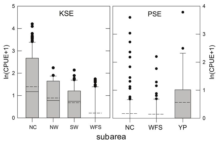
76                         Bulletin of Marine Science. Vol 99, No 2. 2023

Figure 3. Relative abundance [ln(CPUE+1)] of king snake eel (KSE) and palespotted eel (PSE)
sampled in the Gulf of Mexico, 2011–2017. Data are separated by subarea (Fig. 1) where NC =
North Central, NW = Northwest, SW = Southwest, WFS = West Florida Shelf, and YP = Yucatán
Platfom. CPUE is the number of fish caught 1000 hook hrs−1. Solid horizontal lines in each bar
are the medians, averages are horizontal dashed lines. Gray bars are interquartile ranges.

(accounting both for the numbers of hooks fished and set duration) was 1.24, and
thus adjusted catches were similar, on average, to the nominal catches obtained at
each station.

   Species Demography.—Population demographic information, including size dis-
tributions, relative abundance indices (CPUE, as above), length-weight relationships,
and environment-fish interrelationships were calculated for all specimens captured,
and in some cases, for subregions of the GoM, following Murawski et al. (2018). That
paper divided the GoM into six subregions based on consistent variations in fish
community assemblage structure using similarity profile (SIMPROF) tests (Fig. 1) of
species compositions by longline set. We tested main effects for relative abundance
of KSE and PSE among appropriate subareas using analysis of variance (ANOVA)
with raw CPUE data and data transformed as: ln[CPUE+1] (Fig. 3). For KSE we had a
time series of six annual surveys (2011–2017) in the north central (NC) GoM which
we tested for year main effects with ANOVA (Fig. 4).
   Size frequency data for KSE (Table 1) were contrasted for subareas where they were
found (Fig. 5), but there were insufficient samples of PSE (Table 2) for a similar re-
gionally disaggregated comparison (Fig. 6). Length-weight relationships were fit for
both species and for spatial subsets for KSE (i.e., NC, NW, SW GoM) with an expo-
nential model (TW = α*TLβ) where α, β are regression coefficients, TL is total length
in cm and TW is total weight in kg (Fig. 7). The slopes and adjusted means of length-
weight regressions for KSE among the three subareas were tested for significant dif-
ferences using analysis of covariance (ANCOVA).
Murawski and Gracia: Spatial ecology of eels in the Gulf of Mexico                      77

Figure 4. Relative abundance [ln(CPUE+1)] of king snake eel (KSE) sampled in six years in the
North Centeral (NC) area (Fig. 1) of the Gulf of Mexico, 2011–2017. CPUE is the number of fish
caught 1000 hook hrs−1. Solid horizontal lines in each bar are the medians, averages are horizon-
tal dashed lines. Gray bars are interquartile ranges.

  Distribution on Environmental Continua and Species Overlap
Calculations.—How do species array along common environmental gradients
used to describe main niche environmental axes of demersal fishes (e.g. bottom tem-
perature, water depth, etc.)? How can such information be used to predict where the
species are located spatially and how they may interact? Species distribution models

Table 1. Size characteristics [total length (cm), total weight (kg)] of king snake eels sampled from the Gulf of
Mexico, 2011–2017. Subarea designations are as per Figure 1.

Characteristic/Subarea           Number            Mean              SD           Minimum         Maximum
Total Length (cm)
    All Areas                     1413           138.62            42.69             32              226
    North Central                 1271           141.27            42.46             49              226
    Northwest                       48           121.38            45.71             71              200
    Southwest                       64           111.25            34.73             32              204
Total Weight (kg)
    All Areas                     1413              5.81            4.83              0.14             18.4
    North Central                 1271              6.03            4.84              0.14             18.4
    Northwest                       48              4.72            5.42              0.48             18.4
    Southwest                       64              3.05            3.19              0.31             14.2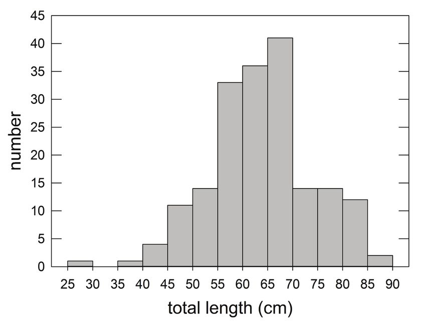
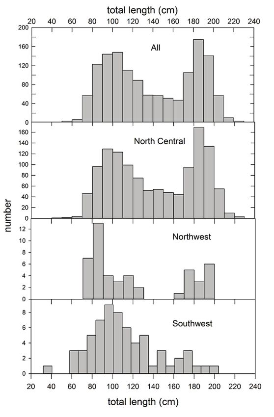
78                         Bulletin of Marine Science. Vol 99, No 2. 2023

Figure 5. Size composition (total length, cm) of king snake eels sampled with longline gear in
the Gulf of Mexico, 2011–2017. Data are presented for all subareas combined, and for the North
Central, Northwest, and Southwest subareas (Fig. 1).
Murawski and Gracia: Spatial ecology of eels in the Gulf of Mexico                        79

Table 2. Size characteristics [total length (cm), total weight (kg)] of palespotted eels sampled from the Gulf of
Mexico, 2011–2017. Subarea designations are as per Figure 1.

Characteristic/Subarea           Number            Mean              SD           Minimum          Maximum
Total Length (cm)
    All Areas                      183             63.26            10.38             27                88
    North Central                   14             55.43             6.47             43                66
    Northwest                       96             62.62            10.97             27                85
    Southwest                       73             65.62             9.38             35                88
Total Weight (kg)
    All Areas                      184              0.32             0.17              0.02              1.07
    North Central                   14              0.21             0.08              0.10              0.32
    Northwest                       97              0.30             0.15              0.02              0.83
    Southwest                       73              0.36             0.19              0.06              1.07

have become an essential tool in understanding abiotic and biotic controls on spatial
distributions leading to their use in forecasting distributional responses to climate
change and understanding effects of marine protected areas (MPAs), among other
uses (Guisan and Thuiller 2005, Poggiato et al. 2021). More generally, multispecies
distribution models (MSDMs) and joint species distribution models (JSDMs) were
introduced to overcome the assumption of species distribution models (SDMs) that
species’ distributions are independent of each other (Poggiato et al. 2021).
  In order to evaluate how fishes partition along habitat characteristics we used
environmental covariates collected during the longline sets. We averaged bottom

Figure 6. Size composition (total length, cm) of palespotted eels sampled with longline gear in
the Gulf of Mexico, 2011–2017.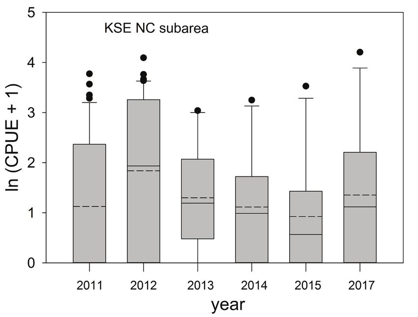
80                          Bulletin of Marine Science. Vol 99, No 2. 2023

                  A

                  B

Figure 7. (A) Total length (cm) – total weight (kg) relationship for king snake eels sampled in
the Gulf of Mexico, 2011–2017. Black line is the least squares nonlinear regression estimator
described by TW = 0.0000024487 TL2.9337, R2 = 0.9437 (P < 0.0001). Also plotted is the similar
regression line obtained by Clark (2000). (B) Total length (cm) – total weight (kg) relationship
for palespotted eels sampled in the Gulf of Mexico, 2011–2017. Black line is the least squares
nonlinear regression estimator described by TW = 0.00000052409 TL3.1897, R2 = 0.8301, P < 0.05.
Murawski and Gracia: Spatial ecology of eels in the Gulf of Mexico 81
Table 3. Mean (unweighted and weighted by CPUE), standard deviation (SD), and coefficient of variation
(CV) of depth (m) and bottom water temperature (°C) at capture of king snake eel and palespotted eel in the
Gulf of Mexico longline surveys, 2011–2017.
Statistic Depth (m) Temperature (°C)
Mean SD CV Mean SD CV
King snake eel
Unweighted 162.55 76.12 0.47 16.81 3.50 0.21
Weighted 168.72 58.12 0.34 15.95 2.71 0.17
Palespotted eel
Unweighted 129.31 65.53 0.51 18.13 3.25 0.18
Weighted 162.18 45.76 0.28 16.81 2.28 0.14
All Stations Sampled
Unweighted 157.51 111.35 0.71 18.24 4.68 0.26
temperatures and water depths from the beginning and end points of each set (Table
3). Distributions of KSE and PSE along these variables were plotted for the entire re-
gion and for relevant subareas (Figs. 8 and 9). Mean, median, standard deviation (SD),
and coefficient of variation (SD/mean) were computed two ways: by weighting the
occurrence of the species at each positive catch location by CPUE (weighted method)
and by using just the series of positive catch locations (without weighting).
A hierarchical series of SMDs were fitted using generalized additive models
(GAMs) for each species independently employing various subsets of environmen-
tal covariates to predict positive occurrences of each species. Independent variables
included in preliminary GAM model fits were average water depth (m) of each set,
average bottom temperature (°C), latitude, longitude, and bottom sediment type,
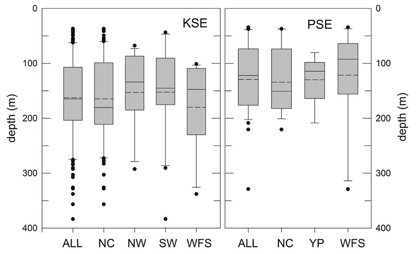
Figure 8. Depth distributions (average depths, unweighted by relative abundance) of catches of
king snake eel (KSE) and palespotted eel (PSE) sampled from the Gulf of Mexico, 2011–2017.
Data are presented for all subareas (Fig. 1) as well as for the North Central (NC), Northwest
(NW), Southwest (SW), West Florida Shelf (WFS), and Yucatán Platform (YP). Solid horizontal
lines in each bar are the medians, averages are horizontal dashed lines. Gray bars are interquar-
tile ranges.82 Bulletin of Marine Science. Vol 99, No 2. 2023
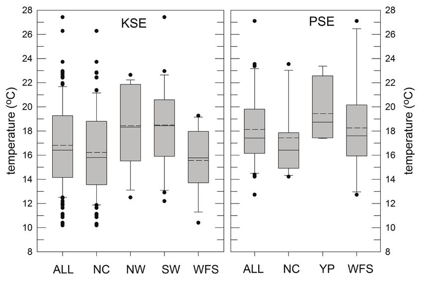
Figure 9. Bottom temperature distributions (average temperatures, unweighted by relative abun-
dance) of catches of king snake eel (KSE) and palespotted eel (PSE) sampled from the Gulf of
Mexico, 2011–2017. Data are presented for all subareas (Fig. 1) as well as for the North Central
(NC), Northwest (NW), Southwest (SW), West Florida Shelf (WFS), and Yucatán Platform (YP).
Solid horizontal lines in each bar are the medians, averages are horizontal dashed lines. Gray
bars are interquartile ranges.
individually and in various combinations. Bottom sediment types associated with
each longline set location were determined in one of four ways.
1. For some stations, bottom type was determined directly by deploying either a
multicorer (eight simultaneous cores) or surficial sediments collected using a
Shipek sediment grab during some of our sampling cruises.
2. For those stations not directly sampled, we located the nearest available point
as summarized in the usSEABED database for the Gulf of Mexico (Buczkowski
et al. 2006; Fig. 10). Using the usSEABED data we used sediment grain size
(ϕ-unit, log2) averages to classify sediments into two broad types: sand ϕ = −1
to 4.0, silt-mud = 4.1 to 8.0 (Fig. 10). Clay substrates are characterized by ϕ =
8.1 to 10.0, but few clay-dominated samples were included in the data set and
are so deleted from analysis and mapping.
3. For the Mexican GoM we used recent sediment data recorded in several cruis-
es that covered continental shelf and deep waters of the South GoM (Gracia
2010) when these samples were located near our longline stations.
4. If sediment samples were not proximate to our station locations, we used gen-
eralized continental shelf surficial sediment maps published by Uchupi and
Emory (1968), Balsam and Beeson (2003), Chanton et al. (2009), and Darnell
(2015) to determine the most likely sediment type associated with each re-
maining station. Because neither KSE or PSE were caught in stations sampled
off northwest Cuba, and adults of neither species had been reported there
(Claro et al. 2001), we eliminated those 30 stations from our modeling data set.Murawski and Gracia: Spatial ecology of eels in the Gulf of Mexico 83 Figure 10. Distribution of longline sampling catches of king snake eel and palespotted eel and surficial sediment samples in the North Central subarea of the Gulf of Mexico during 2011–2017. Isobaths are in 100 m intervals from 100 to 1000 m. DWH is the site of the 2010 Deepwater Horizon oil spill. Surficial sediment characterization from samples obtained by the US Geological Survey and published by Buczkowski et al. (2006). Numerical data are expressed as the average ϕ-unit (log2) mean sediment grain size, converted to characterizations: sand ϕ = −1 to 4.0, silt- mud = 4.1 to 8.0. GAM models were fitted using the mgcv package (Wood 2017, 2022), as imple- mented in R (R Development Core Team 2020). Our GAMs incorporated both non- linear smoothers (splines) and a factor-based independent variable (sediment type). Average depth and average bottom temperature were highly negatively correlated in our station data (R2 = 0.66, P < 0.01). We thus chose to eliminate water temperature from our candidate list of predictor variables as temperature and depth are colinear. Because water depth at a particular location would presumably not vary, as opposed to temperature, depth may be a better predictor of distribution for the presumably nonmigratory benthic adult stages of these species. Latitude was also eliminated be- cause of the complex relationship with abundance for both species (Fig. 2). Candidate GAM models and their permutations thus incorporated three predictor variables: ρi,j = f(Sedimentj) + s(Depthj) + s(Longitudej) + εi,j where ρi,j is the occurrence of species i (0,1) at station j, f() indicates a categorical factor descriptor (i.e., for Sediment) at station j, the s()’s indicate numerical descriptors fit as smoothing splines for depth and longitude at station j, and εi,j is an error term. Presence/absence of each species was used as the dependent variable as
84                                    Bulletin of Marine Science. Vol 99, No 2. 2023

Table 4. Fitting of general additive models (GAMs) for king snake eel (KSE) and palespotted eel (PSE) in the
Gulf of Mexico. Presence-absence of each species is modeled assuming a binomial error distribution with a
logit link function. Independent variables are water depth (D), longitude (Long), and surficial sediment type
(S). AIC is the Akaike Information Criterion, R2 is the coefficient of determination. * = P < 0.05, ** = P <
0.01, *** = P < 0.001, ns = nonsignificant.

Independent Variables               AIC / R2      Significance of            Significance of Nonparametric
                                                  Parametric Effects (Z)     Effects (χ2)
King snake eel
    D, Long, S                  255.6 / 0.50      S = 6.394 ***              D = 48.91 ***, Long = 24.82 ***
    D                           366.9 / 0.20      ---                        D = 53.3 ***
    Long                        365.9 / 0.19      ---                        Long = 24.86 **
    S                           353.5 / 0.25      S = 8.322 ***              ---
    D, Long                     296.2 / 0.40      ---                        D = 50.78 ***, Long = 31.09 ***
    D, S                        284.5 / 0.42      S = 8.129 ***              D = 47.82 ***
    Long, S                     331.6 / 0.30      S = 6.182 ***              Long = 17.93 ***
Palespotted eel
    D, Long, S                  159.1 / 0.22      S = −3.307 ***             D = 6.87 ns, Long = 18.239 **
    D                           203.0 / 0.02      ---                        D = 6.25 ns
    Long                        177.7 / 0.11      ---                        Long = 16.10 *
    S                           203.5 / 0.02      S = −2.68 **               ---
    D, Long                     170.7 / 0.16      ---                        D = 6.22 ns, Long = 16.26 *
    D, S                        196.9 / 0.05      S = −2.827 **              D = 7.178 ns
    Long, S                     168.9 / 0.14      S = −3.038 **              Long = 18.28 *

we also examined the probability of species co-occurrence (a bivariate metric). We
fit a number of GAMs for each species using all combinations of one, two, and three
independent variables (Table 4) to better understand the relative contributions of
the independent variables to the overall model fits. Model fits were evaluated based
on the statistical significance of parametric and nonparametric (smoothed) effects
and overall relative model fits as indexed by the Akaike Information Criterion and
the coefficient of determination (R2; Table 4). Predicted smoothing functions and
linear factor estimates and their 95% confidence limits are plotted over the ranges of
sampled depths, longitudes, and sediments (Fig. 11).
   A number of previous studies (e.g., Murawski and Finn 1988, Turner et al. 2017)
have used environmental covariates in first order SDMs to predict the probability of
two (or more) species co-occurring. In general form, overlap integrals (May 1973) for
two or more species (i,j) along a resource continuum can be computed as:

     αi,j = ∫ f i (x) f j (x) dx.

   These data can follow a number of statistical distributions, but most commonly
fishes are normally or log-normally distributed along these environmental gradients.
Assuming Gaussian (normal) distribution along a resource continuum allows the
use of the normal distribution function to compute the intersections of n species
co-distributions:

     αi,j = Ci,j exp[−d2/2(ωi2 + ωj2)], and

     Ci,j = (2ωiωj/(ωi2 + ωj2))½
Murawski and Gracia: Spatial ecology of eels in the Gulf of Mexico 85
A B C
D E F
Figure 11. Generalized additive model (GAM) results for king snake eel presence/absence, as
a function of water depth (A), longitude (B), and sediment type (C) based on longline survey
data collected in the Gulf of Mexico, 2011–2017. Generalized additive model (GAM) results for
palespotted eel presence/absence, as a function of water depth (D), longitude (E), and sediment
type (F). Smoothing functions (S) of depth and longitude are plotted for both species as are the
relative effects estimates for two values (sand, mud/silt) for the sediment variable (sand is the
standard = 0). Dark lines are estimates of smoothing functions, dashed lines or shading are 95%
confidence limits of estimates.
where: αi,j = the overlap coefficient between species i and j, d = “distance” between
mean environmental values for species i and j, and ωi, ωj = the standard deviations
of the distributions of species i and j along environmental continua (May 1973,
Murawski and Finn 1988). We computed αi,j values for overlap in temperature and
depth of occurrence separately for KSE and PSE and related these coefficients to the
actual percentage of longline sets where co-occurrence of both species occurred.
Effects of depth on the size of animals captured were assessed via linear regression
of size (total length, cm) on average depth of capture (m).86 Bulletin of Marine Science. Vol 99, No 2. 2023
Results
KSE were captured throughout the western GoM from Cape San Blas off the
northwest Florida coast to Campeche Canyon off Mexico (Figs. 1 and 2). Significant
ANOVA subarea main effects (P < 0.01) confirmed differences in CPUE throughout
the GoM. Average CPUE was highest in the north central (NC) GoM, with progres-
sive declines in catch rates in the northwest (NW) and southwest (SW; Fig. 3). Some
KSE were taken on the West Florida Shelf (WFS) just east of DeSoto Canyon (Figs. 1
and 2), but CPUE there was low (Fig. 3). No KSE were captured in longline sets on the
Yucatán Platform or off Cuba (Fig. 2). Repeated sampling in the NC region from 2011
to 2017 (no survey in 2016) revealed a declining trend in average CPUE between 2011
and 2015, but main effects for year were not significant (P > 0.05).
PSE also demonstrated a significant subarea effect in CPUE (Fig. 3; ANOVA, P <
0.01) but they were absent in our collections from the NW, SW, and Cuba. PSE were
most abundant on the Yucatán Platform and found in lower densities along the WFS
and in the eastern portion of the NC subarea (Figs. 2 and 3).
A total of 1414 KSE and 190 PSE were sampled on the 343 longline sets (313 sets
outside Cuba; Tables 1 and 2). Average total length of KSE was 139 cm, with a maxi-
mum of 226 cm, the longest TL for the species yet reliably reported (e.g., Clark 2000;
NB, Clark 2000 mistakenly used the common name giant snake eel despite king
snake eel being the accepted common name by the American Fisheries Society at the
time Clark’s study was published (Robins et al. 1991)). Little has been published on
the biology of KSE, with Clark’s (2000) study being the only one providing life history
parameters for the species. KSE in our study averaged 5.8 kg TW with the heaviest
fish being 18.4 kg. In contrast, PSE averaged 63 cm and 0.3 kg, demonstrating a two-
fold difference in average TL and an 18-times difference in average TWs between the
two species. Maximum TL and TW differed by 2.5 and 17 times respectively for the
two species.
The overall size composition of KSE (Fig. 5) was bimodal, perhaps reflecting di-
morphic growth rates between females (larger asymptotic lengths) and males (Clark
2000). The combined size composition of sampled KSE primarily reflects fish cap-
tured in the NC subarea, as sampling effort there (number of sets) was six times the
number of stations sampled in the NW subarea and three times the stations sampled
in the SW (Fig. 2), and the average CPUE in the NC was larger than in the other
two areas (Fig. 3). KSE sampled in the NW also demonstrated a bimodal distribu-
tion, although it was based on fewer fish. In the SW subarea, fish distributions were
unimodal with a long right-hand tail. Average lengths of KSE progressively declined
from 141 cm in the NC to 121 cm in the NW and 111 in the SW; weights reflected a
similar pattern (Table 1). The minimum size of KSE captured by the gear was 32 cm
but few animalsMurawski and Gracia: Spatial ecology of eels in the Gulf of Mexico 87 Length-weight equations for the two species (Fig. 7) indicate that KSE were, on av- erage, 56% heavier at a given length than PSE over the majority of the PSE size range (60–85 cm). For KSE the total length-total weight relationship from Clark (2000) was overplotted with the current values indicating little difference between them despite sampling that was separated by over two decades (1988–1989 vs 2011–2017; Fig. 7, top panel). Length-weight equation slopes (β) for KSE differed among subareas (NC, NW, SW; ANCOVA: P < 0.01) but predicted weights at length were similar among subareas. Both KSE and PSE were distributed in mid- to outer-shelf waters (Fig. 2) with aver- age depths (weighted by fish catch) of 169 and 162 m, respectively, at mean bottom water temperatures of 16 and 16.8 °C, respectively (Table 3, Figs. 8 and 9). There were no significant differences in depth at capture by subarea for either species (P > 0.05; Figs. 8 and 9) although temperatures at capture did vary likely due to seasonal differ- ences in times of collection. Consistent with similarities in depths and temperatures at capture, overlap co- efficients (αi,j) were relatively high [temperature: 0.9643 (weighted) and 0.9612 (un- weighted), depth: 0.9821 (weighted) and 0.9414 (unweighted)]. However, despite the similarities in average depth and bottom water temperature at capture and the re- sulting high overlap coefficients between KSE and PSE, both species co-occurred in longline catches at only 4 of 343 (0.012) of the stations sampled. If stations where only one or both of the species are analyzed, the proportion where they co-occurred is only (4/172) = 0.023. Clearly other environmental determinants besides temperature and depth are more influential in habitat selection and differentiation between KSE and PSE. The GAM modeling results (Fig. 11) depict both the estimated effects for the factor class “sediment” as the right hand panels of the graphs for KSE and PSE and the esti- mated (and additive) smoothing functions for presence/absence by depth and longi- tude in the right and center panels. The effects modeling uses a standard class (in this case “sand”) and estimates the relative effects for “mud/silt” for both KSE and PSE. Smoothing functions (S) provide spline functions describing the relationship of each continuous predictor variable on overall presence/absence of each species (Fig. 11). Results of GAM modeling reflect a high degree of predictability for KSE presence/ absence: all environmental predictor variables were highly significant (P < 0.001) in one, two, and three parameter model configurations (Table 4). The lowest AIC (255.6) and highest model coefficient of determination (0.50) resulted from the inclusion of water depth, longitude, and sediment type (Table 4, Fig. 11) as independent variables. Lowest R2 values (and highest AICs) resulted from single independent variable fits (D, Long, S), followed by the two parameter models (D+Long, D+S, Long+S). Nonlinear model smooths for KSE (Fig. 11, top panels) show a strong hyperbolic shape to depth at capture over the sampled depth range of the species (Fig. 8). The longitude smooth- er peaks at roughly 89°W, consistent with the peak in abundance in the NC region (Fig. 2). The model parameters for the sediment factor indicate a strong affinity of KSE for mud/silt habitats as compared with sand habitats (Fig. 11, top left) and the number of locations sampled with mud/silt bottom sediment were comparatively larger than sand habitats that were mainly found on the Yucatán Platform and West Florida Shelf. GAM results for PSE again indicated that the best model fits were for the three- parameter configuration (AIC = 159.1, R2 = 0.22) but the depth variable smooths were
88                        Bulletin of Marine Science. Vol 99, No 2. 2023

nonsignificant in all one, two, and three independent model cases (Table 4, Fig. 11
bottom panels). As with KSE, the sediment factor was highly significant in all model
fits with the species demonstrating a high affinity for sand habitats, in contrast to
KSE (Fig. 11). The overall model fits were less precise for PSE vs KSE which may re-
flect the fact that PSE were caught in only 32 of the stations whereas KSE were caught
in 144 longline sets (Fig. 2).

                                        Discussion

   Despite being taken as directed and bycatch in commercial fisheries (e.g., Barton
et al. 1988, Scott-Denton et al. 2011, 2012, Castro-González et al. 2012) and, in the
case of KSE, in recreational fisheries, little published ecological or habitat informa-
tion is available for KSE or PSE. Although not targeted in US fisheries (primarily for
KSE due to the presence of numerous bones in the fillets), both species are frequent-
ly caught as bycatch in bottom longline fisheries in the GoM with 29% and 11% of
catches of KSE and PSE retained for use as bait (Scott-Denton et al. 2011). Reflecting
the general lack of life history information for the species, KSE was only described
as a unique species in 1980 (Böhlke and Caruso 1980). In their original description,
the holotype and paratypes for KSE cited by Böhlke and Caruso did not include any
specimens from Mexican waters, although distributions have been reported there
(Espinosa et al. 2008, Castro-González et al. 2012). The PSE was described in 1859,
originally under the genus Cryptopterus, although again little ecological information
has been published on the species other than their occurrences in larval collections
(Fahay and Obenchain 1978, Miller and McCleave 2007, Moore et al. 2020).
   A series of 12 scientifically-based longline surveys conducted after the 2010
Deepwater Horizon oil spill sampled the north central Gulf of Mexico over a period
of seven years and extended longline surveys to all continental shelves of the Gulf
of Mexico (Murawski et al. 2018). KSE and PSE were dominant components of fish
assemblages sampled throughout the GoM, with species abundance (CPUE) varying
by subregion (Figs. 1–3). A total of 1414 KSE and 190 PSE were sampled during those
surveys and they provide the material upon which this study is based.
   Neither species was sampled in 30 longline sets conducted along the northwest
coast of Cuba (Fig. 2) despite the presence of PSE leptocephalii in waters of the Florida
Straits (Moore et al. 2020). Northwest Cuban waters have a steep bathymetry and are
dominated by shallow-water and mesophotic coral reefs (Claro et al. 2001) with lim-
ited sand or mud habitats in the depth ranges where KSE and PSE were encountered
elsewhere in the GoM. Thus, there may be little optimal bottom habitat available for
adults of either species to recruit along the NW Cuban coast.
   Although primarily distributed on the continental shelves as adults, leptocepha-
lus larval stages of KSE and PSE occur in deep waters of the central GoM (>1000 m;
Collins 2019, Moore et al. 2020). Prominent current systems in the GoM (e.g., the
Loop Current) and ephemeral transport mechanisms including cyclonic and anti-
cyclonic eddies from the Loop Current thus may potentially distribute KSE and PSE
larvae widely in the GoM. Consistent with this hypothesis, for KSE no apparent spa-
tial structure was evident using DNA from fin clips of adults sampled from Mexican
and US waters (Chavez et al. 2022). Thus, given the putative protracted leptocephalus
larval stages for ophichthids, including KSE and PSE (Collins 2019) and their larval
distribution in deep waters of the central GoM (Moore et al. 2020), the high degree
Murawski and Gracia: Spatial ecology of eels in the Gulf of Mexico 89 of connectivity among adult stages is likely maintained by extensive larval transport by prevailing and episodic currents (Collins 2019). Since no tagging studies of either species have been reported, it is unclear if adults or demersal juveniles undertake extensive movements or migrations. Statistically significant increases in average size of both KSE and PSE with increasing water depth (our results) may either indicate ontogenetic movement of larger adults to deeper water or, conjecturally, increased mortality in nearshore waters subject to intensive fishing and other stressors. In any event, movement studies would be valuable to deconvolve these processes. Differences in the distribution and relative abundance of KSE and PSE across subareas of the GoM are apparently due primarily to the differential occurrence of preferred sediment habitats. These two species share similar depth and bottom tem- perature envelopes as demersal juveniles and adults (Table 3, Figs. 8 and 9), but were caught together in very few instances. KSE were found almost exclusively in mud/silt habitats and PSE on sand bottoms, and these differences are apparent in the GAM modeling (Table 4, Fig. 11). The four instances where the two species were caught together were in the NC region west of DeSoto Canyon (Fig. 10). This region repre- sents the transition zone between sand sediments that predominate on the WFS and mud sediments characteristic of areas further west (Fig. 10; Uchupi and Emory 1968, Balsam and Beeson 2003, Chanton et al. 2009, Darnell 2015). East and southeast of Cape San Blas shelf sediments are primarily carbonate sand, with the exception of quartz sand in nearshore waters (Balsam and Beeson 2003) derived from weathering and transport from the southern Appalachian Mountains (Darnell 2015). East of the Mississippi Delta to Cape San Blas (Figs. 1 and 10) the basal sea floor is primarily quartz sand and is referred to as the MAFLA (Mississippi-Alabama-Florida) Sand Sheet (Balsam and Beeson 2003). More modern sediments derived from terrigenous inputs (primarily from the Mississippi River Delta) overlay the MAFLA Sand Sheet resulting in the complex pattern of sediments seen in the region (Fig. 10). In this area some of the MAFLA is surficial west of DeSoto Canyon, whereas pockets of mud/silt sediments and marl extend east of the Canyon. Resultantly, the distributions of PSE and KSE can vary considerably over relatively short distances (Fig. 10). Given that our longline sets were 8 km in length, it is possible that for the few sets where both species were caught there was sufficient habitat heterogeneity resulting in apparent co-occurrence. Surficial sediments west of the Mississippi Delta to along the Texas Shelf are pri- marily terrigenous muds with a number of offshore sand banks and, in the south- ern part of the region, salt diapirs overlain primarily with sand (Balsam and Beeson 2003, Darnell 2015). As well there are some nearshore sand deposits. While we only sampled KSE in the shelf waters off Texas, the location of sand patches within this region explains some reports of PSE in the area (STRI 2022). In the southwest GoM (to Campeche Canyon) sediments are dominated by terrigenous muds (Uchupi and Emory 1968) with some intermittent sand deposits. The Yucatán Platform is over- lain by calcareous sands in shallow areas and calcareous oozes offshore (Balsam and Beeson 2003, Chanton et al. 2009); the Platform is interspersed with living and fossil- ized coral reefs (Darnell 2015). The high densities of PSE and absence of KSE on the Yucatán Platform are consistent with the hypothesized regional habitat partitioning and bottom type preferences between the species. Despite the similarity of depth and temperature envelopes occupied by the two eel species, spatial separation associated with differing bottom type preferences also
90                        Bulletin of Marine Science. Vol 99, No 2. 2023

resulted in vastly different fish species associates in their respective assemblages.
Murawski et al. (2018) conducted SIMPROF analyses of station groupings and
corresponding species associations from the longline samples we also used. In
their analyses, king snake eel was most closely associated with gulf smoothhound
Mustelus sinusmexicanus, yellowedge grouper Hyporthodus flavolimbatus, and
wenchman Pristipomoides aquilonaris, and more broadly with southern hake
Urophycis floridana, tilefish Lopholatilus chamaeleonticeps, shortspine dogfish
Squalus mitsukurii, and gulf hake Urophycis cirrata. In contrast, palespotted eels,
occupying predominately sand habitats, were most closely associated with red porgy
Pagrus pagrus, almaco Jack Seriola rivoliana, reticulate moray Muraena retifera,
blackline tilefish Caulolatilus cyanops, and sharksucker Echeneis naucrates, snakefish
Trachinocephalus myops, and ocellated moray eel Gymnothorax ocellatus. The two
species thus interact with very different fish assemblages despite their similar depth
and temperature affinities. Differences in preferred habitat types resulting in distinct
habitat partitioning have likely allowed these two sympatric species to coexist despite
the order of magnitude difference in average body weights between the species
(Tables 1 and 2) and likely antagonistic behaviors between these two omnivorous
predators (NB, based on our experiences both species are highly aggressive when
brought to the surface on longline gear).
   The lack of significant change in abundance of KSE after 2011 in the NC region
(Fig. 4) and the apparent stability in body condition (weights for a given length; Fig.
7) are an enigma because the area significantly overlaps with the distribution of sedi-
mented oil from the 2010 DWH accident (Romero et al. 2017). Polycyclic aromat-
ic hydrocarbons (PAHs) in muscle and liver in KSE sampled following DWH were
much lower than other common demersal fishes (Snyder et al. 2015, 2019, Pulster et
al. 2020) even when these species were captured concurrently with KSE (Murawski et
al. 2014). PAHs in sediments readily bind with fine particulates comprising muds and
clays and thus the likely burrow-forming demersal juvenile and adult KSE should be
continually exposed to relatively high sedimented PAH concentrations in oiled areas
(Romero et al. 2017). In the case of tilefish, (a species often associated with KSE in the
area exposed to DWH oil; Murawski et al. 2018), increasing exposure to petrogenic
PAHs over time was associated with a 22% decline in condition factor (weight for a
given length) and a 53% decline in liver lipid concentration (Snyder et al. 2019). For
KSE, however, there were no significant changes in body condition before and after
the oil spill. Why then were the observed body burdens (in liver, muscle and bile)
for KSE so low and effects on condition so different between tilefish and KSE? One
potential explanation lies in the physiology of KSE. Also known colloquially as “mud
eels” and “slime eels”, our observations are that KSE produce prodigious quantities
of mucous when stressed. Previous laboratory studies have found that mucous pro-
duction represents a pathway for PAH removal following intraperitoneal injection
(Varanasi et al. 1978). It is thus possible (likely) that physiological adaptations of KSE
explain the relatively low body accumulation of PAHs (and potentially other organic
compounds) despite their residues in highly polluted sediments (from anthropogenic
sources and hydrocarbon seeps) of the north central GoM, and thus the persistence
of the KSE population in the area surrounding DWH.
   Size composition data from the NC GoM were available herein and from a study
undertaken in 1988–1989 and published in Clark (2000). In that study there was
likewise a bimodal length frequency (modes at ca 120–130 cm and 180–190 cm).
Murawski and Gracia: Spatial ecology of eels in the Gulf of Mexico    91

Clark found the sex ratio was 4:1 (♀:♂) based on macroscopic examination of gonads.
Age and growth information provided by Clark (2000) indicated strong dimorphic
growth with females attaining a maximum age of 30 years, and males a maximum
of 17 years. All fish >180 cm TL were female in Clark’s study. We undertook macro-
scopic examinations of fresh caught KSE specimens in the field with very different
results. Overall, we found a sex ratio of 1.08:1 (♀:♂), with females only dominating
in the largest size class (210–226 cm). However, our sampling was done primarily in
late spring and summer when spawning had apparently ceased, and most animals
were in resting or recovering gonadal development stages. Given these disparities,
more detailed microscopic sex determinations are recommended in future popula-
tion studies involving KSE.
   KSE from the NC, NW, and SW subareas showed a progressive reduction in mean
size along this N–S continuum. This could either indicate a bias in sampling locations
against areas occupied by large animals in the more southern areas or more likely
differences in mortality and/or growth rates of the species. While length-weight re-
lationships were statistically different among the three areas, predicted weights at
length were similar indicating that differences in average lengths among the areas do
not necessarily reflect differences in average condition of the animals or overall pro-
ductivity. PSE average total lengths were highest on the Yucatán Platform and lower
in the NC and WFS regions. Again, reasons for these differences are unclear but may
be related to either productivity or mortality rates of the species.
   How might these two eel species differentially respond to future warming scenari-
os in the GoM given apparent obligate associations of KSE and PSE with mud/silt and
sand habitats, respectively, and their similar temperature and depth associations?
If GoM coastal waters warm appreciably in the future and the species respond by
seeking deeper waters (a more likely scenario than poleward range extension in semi-
enclosed seas such as the GoM), then are there sufficient preferred sediment habitats
in deeper (i.e., cooler) waters for the species to occupy? In the case of KSE, deeper wa-
ters tend to have sufficient mud/silt/marl sediment seaward of current distributions
to occupy (Figs. 2 and 10; Chanton et al. 2009). However, for PSE, the lack of surficial
sand deposits at the shelf edge and beyond perhaps suggest that warming scenarios
indeed may limit the ability of the species to occupy preferred sediment types, thus
potentially limiting its distribution and increasing interactions with other species
including KSE.

                                    Acknowledgments

   This research was supported by the Gulf of Mexico Research Initiative (GoMRI),
through its Center for Integrated Modeling and Analysis of Gulf Ecosystems (C-IMAGE),
via Grant NA11NMF4720151 – Systematic Survey of Fish Diseases in the Gulf of Mexico,
from the National Marine Fisheries Service (NMFS), NOAA, and by the Louisiana Oil Spill
Coordinator’s Office (LOSCO). Our longline sampling was conducted aboard the fishing ves-
sels Pisces, Sea Fox, and Brandy and the research vessel Weatherbird II, operated by the
Florida Institute of Oceanography and we appreciate the skilled efforts of captains, crews,
and scientists aboard and especially our “Mud and Blood” crews. The US National Marine
Fisheries Service provided appropriate sampling authorizations and technical guidance.
Sampling was in accordance with approved Institutional Animal Care and Use Committee
(IACUC) protocol IS00000515, authorized by the University of South Florida. We also thank
the USA and Mexican Departments of State, PEMEX, SEMARNAT, and CONAPESCA, the
92 Bulletin of Marine Science. Vol 99, No 2. 2023
Cuban Ministry of Foreign Affairs (MINREX), the US Departments of Commerce (BIS) and
Treasury (OFAC), and the US Coast Guard for permitting data collection activities. Data
are publicly available through the Gulf of Mexico Research Initiative Information & Data
Cooperative (GRIIDC) at: https://data.gulfresearchinitiative.org (https://doi.org/10.7266/
N7G73C4N). Special thanks are due to the two anonymous reviewers of the manuscript. We
dedicate this contribution to the memories of our colleagues and friends Bill Hogarth, Dave
Hollander, and Wes Tunnell.
Literature Cited
Able KW, Allen DM, Bath-Martin G, Hare JA, Hoss DE, Marancik KE, Powles PM, Richardson
DE, Taylor JC, Walsh HJ, et al. 2011. Life history and habitat use of the speckled worm
eel, Myrophis punctatus, along the east coast of the United States. Environ Biol Fishes.
92:237–259. https://doi.org/10.1007/s10641-011-9837-8
Balsam WL, Beeson JP. 2003. Sea-floor sediment distribution in the Gulf of Mexico. Deep Sea
Res Part I Oceanogr Res Pap. 50:1421–1444. https://doi.org/10.1016/j.dsr.2003.06.001
Barton LE, Otwell S, Burgess GN Jr. 1988. Research and marketing developments for the Rex Eel
Ophichthus rex. Tropical and Subtropical Fisheries Technological Society of the Americas.
Conference Proceedings, October 16-18, Gulf Shores, Alabama. Florida Sea Grant College
Program. SGR-94.
Böhlke JE, Caruso JH. 1980. Ophichthus rex: a new giant snake eel from the Gulf of Mexico.
Proc Acad Nat Sci Philadelphia. 132:239–244.
Buczkowski BJ, Reid JA, Jenkins CJ, Reid JM, Williams SJ, Flocks JG. 2006. usSEABED: Gulf
of Mexico and Caribbean (Puerto Rico and U.S. Virgin Islands) offshore surficial sediment
data release. US Geological Survey Data Series 146 v1.0. 50 p.
Castro-González MI, Maafs-Rodríguez AG, Pérez-Gil Romo F. 2012. Evaluación de diez espe-
cies de pescado para su inclusión como parte de la dieta renal, por su contenido de proteína,
fósforo y ácidos grasos. Arch Latinoam Nutr. 62(2):127–136.
Chanton J, Lapham L, Bianchi TS, Rogers K, Hollander D, Joye S. 2009. Marine sediment
chemistry. In: Bianchi TS, et al., editors. Gulf of Mexico: origin, waters and biota. Volume 5,
chemical oceanography. College Station: Texas A&M University Press. p. 216–233.
Chavez AT, O’Leary S, Cotton C, Murawski S, Portnoy DS. 2022. Large and fine-scale genet-
ic structure of king snake eels (Ophichthus rex) throughout the Gulf of Mexico. Student
Research Symposium Presentation. Texas A&M University Corpus Christi. Available from:
https://tamucc-ir.tdl.org/handle/1969.6/90570
Clark ST. 2000. Age, growth and distributions of the giant snake eel, Ophichthus rex, in the Gulf
of Mexico. Bull Mar Sci. 67:911–922.
Claro R, Lindeman KC, Parenti LR, editors. 2001. Ecology of the marine fishes of Cuba.
Washington DC: Smithsonian Institution Press.
Collins L. 2019. Distribution, abundance, and trophic ecology of anguilliform Leptocephali
in the northern Gulf of Mexico. Master’s Thesis, University of Southern Mississippi 687.
Available from: https://aquila.usm.edu/masters_theses/687
Darnell R. 2015. The American Sea: a natural history of the Gulf of Mexico. College Station,
Texas: Texas A&M University Press.
Espinosa PH, Huidobro L, Flores-Coto C, Fuentes-Mata P, Funes-Rodríguez R. 2008. Catálogo
taxonómico de especies de México. Capital natural de México, vol. I (CD1). [In Spanish]
https://doi.org/10.13140/RG.2.1.1097.6888
Fahay MP, Obenchain CL. 1978. Leptocephali of the ophichthid genera Ahlia, Myrophis,
Ophichthus, Pisodonophis, Callechelys, Letharchus, and Apterichtus on the Atlantic conti-
nental shelf of the United States. Bull Mar Sci. 28:422–486.
Fricke R, Eschmeyer WN, Van der Laan R. 2023. Eschmeyer’s catalog of fishes: genera, spe-
cies, references. California Academy of Sciences. Available from: http://researcharchive.
calacademy.org/research/ichthyology/catalog/fishcatmain.aspMurawski and Gracia: Spatial ecology of eels in the Gulf of Mexico 93 Gracia A. 2010. Campaña oceanográfica (SGM 2010). 2010. Informe Final. Gerencia de Seguridad Industrial, Protección Ambiental y Calidad, Región Marina Noreste, PEMEX- Exploración y Producción, México. Instituto de Ciencias del Mar y Limnología, UNAM. [In Spanish] Guisan A, Thuiller W. 2005. Predicting species distribution: offering more than simple habitat models. Ecol Lett. 8:993–1009. https://doi.org/10.1111/j.1461-0248.2005.00792.x Hastie T, Tibshirani R. 1986. Generalized additive models. Stat Sci. 1:297–318. https://doi. org/10.1214/ss/1177013604 Hastie T, Tibshirani R. 1990. Generalized additive models. Monograph on statistical and ap- plied probability. Boca Raton: Chapman and Hall CRC. May RM. 1973. Stability and complexity in model ecosystems (2nd ed). Monograph on popula- tion ecology. Princeton: Princeton University Press. McEachran JD, Fechhelm JD. 1998. Fishes of the Gulf of Mexico, Volume 1. Austin: University of Texas Press. Miller MJ, McCleave JD. 2007. Species assemblages of leptocephali in the southwestern Sargasso Sea. Mar Ecol Prog Ser. 344:197–212. https://doi.org/10.3354/meps06923 Moore JA, Fenolio DB, Cook AB, Sutton TT. 2020. Hiding in plain sight: elopomorph larvae are important contributors to fish biodiversity in a low-latitude oceanic ecosystem. Front Mar Sci. 7:169. https://doi.org/10.3389/fmars.2020.00169 Murawski SA, Finn JT. 1988. Biological bases for mixed-species fisheries: species co-distribu- tion in relation to environmental and biotic variables. Can J Fish Aquat Sci. 45:1720–1735. https://doi.org/10.1139/f88-204 Murawski SA, Grosell M, Smith C, Sutton T, Halanych K, Shaw R, Wilson CA. 2021. Impacts of petroleum, petroleum components and dispersants on organisms and populations. Oceanography. 34:136–151. https://doi.org/10.5670/oceanog.2021.122 Murawski SA, Hogarth WT, Peebles EB, Barbieri L. 2014. Prevalence of external skin lesions and polycyclic aromatic hydrocarbon concentrations in Gulf of Mexico fishes, post-Deep- water Horizon. Trans Am Fish Soc. 143:1084–1097. https://doi.org/10.1080/00028487.201 4.911205 Murawski SA, Peebles EB, Gracia A, Tunnell JW Jr, Armenteros M. 2018. Comparative abun- dance, species composition, and demographics of continental shelf fish assemblages throughout the Gulf of Mexico. Mar Coast Fish. 10:325–346. https://doi.org/10.1002/ mcf2.10033 Perryman HA, Babcock EA. 2017. Generalized additive models for predicting the spatial distribution of billfishes and tunas across the Gulf of Mexico. ICCAT Coll Vol Sci Pap. 73:1778–1795. Poggiato G, Münkemüller T, Bystrova D, Arbel J, Clark JS, Thuiller W. 2021. On the interpreta- tions of joint modeling in community ecology. Trends Ecol Evol. 36:391–401. https://doi. org/10.1016/j.tree.2021.01.002 Pulster EL, Gracia A, Armenteros M, Toro-Farmer G, Snyder SM, Carr BE, Schwaab MR, Nicholson TJ, Mrowicki J, Murawski SA. 2020. A first comprehensive baseline of hy- drocarbon pollution in Gulf of Mexico fishes. Sci Rep. 10:6437. https://doi.org/10.1038/ s41598-020-62944-6 Quattrini AM, McClain-Counts J, Artabane SJ, Roa-Varón A, McIver TC, Rhode M, Ross SW. 2019. Assemblage structure, vertical distributions and stable-isotope compositions of anguilliform leptocephali in the Gulf of Mexico. J Fish Biol. 94:621–647. https://doi. org/10.1111/jfb.13933 R Development Core Team. 2020. R: a language and environment for statistical computing. Vienna, Austria: R Foundation for Statistical Computing. Available from: http://www.r- project.org/index.html Robins CR, Bailey RM, Bond CE, Brooker JR, Lachner EA, Lea N, Scott WB. 1991. Common and scientific names of fishes from the United States and Canada. 5th ed. Am Fish Soc Spec Publ 20. 183 p.
You can also read