Sugariness prediction of Syzygium samarangense using convolutional learning of hyperspectral images
←
→
Page content transcription
If your browser does not render page correctly, please read the page content below
www.nature.com/scientificreports

                OPEN             Sugariness prediction of Syzygium
                                 samarangense using convolutional
                                 learning of hyperspectral images
                                 Chih‑Jung Chen1, Yung‑Jhe Yan1, Chi‑Cho Huang2, Jen‑Tzung Chien1, Chang‑Ting Chu1,
                                 Je‑Wei Jang1, Tzung‑Cheng Chen3, Shiou‑Gwo Lin4, Ruei‑Siang Shih1 & Mang Ou‑Yang1*

                                 Sugariness is one of the most important indicators to measure the quality of Syzygium samarangense,
                                 which is also known as the wax apple. In general, farmers used to measure sugariness by testing
                                 the extracted juice of the wax apple products. Such a destructive way to measure sugariness is not
                                 only labor-consuming but also wasting products. Therefore, non-destructive and quick techniques
                                 for measuring sugariness would be significant for wax apple supply chains. Traditionally, the non-
                                 destructive method to predict the sugariness or the other indicators of the fruits was based on the
                                 reflectance spectra or Hyperspectral Images (HSIs) using linear regression such as Multi-Linear
                                 Regression (MLR), Principal Component Regression (PCR), and Partial Least Square Regression
                                 (PLSR), etc. However, these regression methods are usually too simple to precisely estimate the
                                 complicated mapping between the reflectance spectra or HSIs and the sugariness. This study presents
                                 the deep learning methods for sugariness prediction using the reflectance spectra or HSIs from the
                                 bottom of the wax apple. A non-destructive imaging system fabricated with two spectrum sensors
                                 and light sources is implemented to acquire the visible and infrared lights with a range of wavelengths.
                                 In particular, a specialized Convolutional Neural Network (CNN) with hyperspectral imaging is
                                 proposed by investigating the effect of different wavelength bands for sugariness prediction. Rather
                                 than extracting spatial features, the proposed CNN model was designed to extract spectral features
                                 of HSIs. In the experiments, the ground-truth value of sugariness is obtained from a commercial
                                 refractometer. The experimental results show that using the whole band range between 400 and
                                 1700 nm achieves the best performance in terms of °Brix error. CNN models attain the °Brix error
                                 of ± 0.552, smaller than ± 0.597 using Feedforward Neural Network (FNN). Significantly, the CNN’s
                                 test results show that the minor error in the interval 0 to 10°Brix and 10 to 11°Brix are ± 0.551
                                 and ± 0.408, these results indicate that the model would have the capability to predict if sugariness
                                 is below 10°Brix or not, which would be similar to the human tongue. These results are much better
                                 than ± 1.441 and ± 1.379 by using PCR and PLSR, respectively. Moreover, this study provides the
                                 test error in each °Brix interval within one Brix, and the results show that the test error is varied
                                 considerably within different °Brix intervals, especially on PCR and PLSR. On the other hand, FNN and
                                 CNN obtain robust results in terms of test error.

                                 The fruit’s quality grading is one of the significant factors in processing agricultural products. A proper procedure
                                 for grading is beneficial to preservation and transportation and increasing the value of the products. The precise
                                 classification and reasonable price make customers willing to purchase the agriculture products. However, the
                                 farmers and dealers subjectively grade the quality and prices of fruits by the product’s size, appearance, color or
                                 sweetness, etc., not precisely because the criterion may not be unified. Syzygium samarangense, also known as wax
                                 apple, for example, the farmers usually determine the sweetness of the wax apple by the color of the peel. With
                                 more scarlet the color is, the more sugar content may be contained within the fruit. However, such judgment is
                                 not only time-consuming but also easily miscalculates the quality of the products. For more precise detection,
                                 auxiliary instruments, such as the °Brix meter or refractometer, have already been developed for detecting the
                                 sugar content. This kind of °Brix meter often utilizes light refraction through the liquid to observe and detect

                                 1
                                  National Yang Ming Chiao Tung University, Hsinchu, Taiwan. 2Fengshan Tropical Horticultural Experiment
                                 Branch, Kaohsiung, Taiwan. 3Feng Chia University, Taichung, Taiwan. 4National Taiwan Ocean University, Keelung,
                                 Taiwan. *email: oym@nctu.edu.tw

Scientific Reports |   (2022) 12:2774                | https://doi.org/10.1038/s41598-022-06679-6                                                   1

                                                                                                                                               Vol.:(0123456789)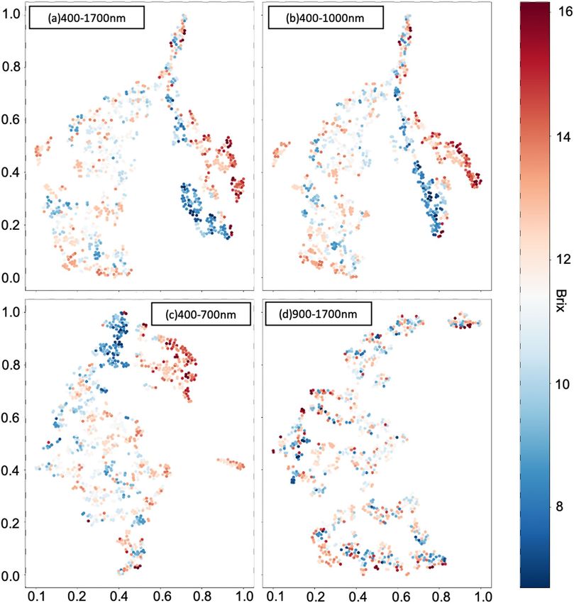
www.nature.com/scientificreports/
Figure 1. The overall workflow for evaluating the related methods in sugariness prediction.
a small detecting error. Additionally, the °Brix obtained from the refractometer is a real number and the sugar
content of an aqueous solution. Usually, one °Brix is 1 g of sucrose 100 g of solution.
Nevertheless, the drawback of the refracted meter is the procedure that needs to destroy the product itself
to extract the juice for detection. This invasive method is not only time-consuming but also impractical for
real applications in the agricultural field. Consequently, the non-destructive sweetness detection technique will
become a crucial issue for measuring the quality of wax apple fruit.
In general, fruit’s non-destructive detecting methods are implemented by analyzing the reflectance spectra
or the Hyperspectral Images (HSIs) of the surface of the fruit. Rather than ordinary RGB images, HSIs would
have more features and be an ideal material to analyze. For instance, previous works presented that hyper-
spectral imaging is more suitable than conventional RGB imaging for evaluating mushroom q uality1, and the
advantages of analysis on HSIs are shown2–4. In the early researches, the analyzing methods including Multiple
Linear Regression (MLR), Principal Component Regression (PCR), and Partial Least Square Regression (PLSR).
Such as the soluble solids content of peaches could be determined using MLR5. The experiments apply PLSR on
the reflectance of apples to detect the fi rmness6, the quality of gala apples could be measured by detecting the
soluble solids and firmness using PCR7. PLSR was used to construct the models to predict glucose, sucrose, and
fructose concentrations in the tubers of potatoes8. The concentration of anthocyanins, polyphenols, and sugar
in grapes was determined using PLSR9. Previous work uses Independent Component Analysis (ICA) and PLSR
to quantify sugar content in wax apple using spectra data with NIR bands (600–1098 nm)10. Moreover, some
proposed researches focus on the nutrients in the wax apple, such as proving that the total anthocyanin content
(TAC) and total phenolic compounds (TPC) were able to be detected by near-infrared spectroscopy11.
In recent years, deep learning is prevalent in developing non-destructive techniques for determining quality
from various fruits. Such as the ripeness of strawberries could be analyzed with CNN and SVM models on HSIs12,
and the maturity of citrus could be estimated with fluorescence spectroscopy data by performing the regression
with a CNN m odel13. Furthermore, deep learning is also broadly applied in the actual farm field. Such as one
of the researches proposed research uses R-CNN based model to detect and count passion fruit in o rchards14,
another implements CNN models on wheat yield f orecasting15, and the other achieves high accuracy on grape
bunch segmentation using deep neural n etworks16.
Those experimental results indicate the potential possibility of using the spectral convolutional neural net-
work to detect the fruit quality. Therefore, take the fundamental requirements from the agricultural field and
the spectral technique’s opportunity into consideration.
Data preparation and evaluation process
Figure 1 shows the workflow of the entire evaluation, which consists of five steps. First, the HSIs of the bot-
tom part of the wax apple were acquired properly and preprocessed as a 1-dimensional array for t-distributed
Stochastic Neighbor Embedding (t-SNE) data visualization, FNN, PCR, and PLSR models, the 3-dimensional
matrix for the 2D-CNN models. Second, t-SNE was used to visualize the dataset to see the distribution of data.
Third, the preprocessed data was split into training, validation, and test datasets. Fourth, the FNN and CNN
models were trained with training and validation datasets.
Furthermore, to review if the clustering results are better than the input samples after the deep learning pro-
cess, t-SNE was applied on the layer’s outputs before the regression output layer. Finally, each model was evaluated
Scientific Reports | (2022) 12:2774 | https://doi.org/10.1038/s41598-022-06679-6 2
Vol:.(1234567890)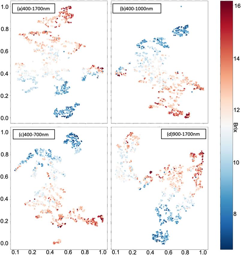
www.nature.com/scientificreports/
with the test dataset, and the error was assessed for different models. Further information on HSIs preprocessing
and modeling in this research will be introduced in the following few parts of this section.
Samples preparation. The most important step is preparing the samples, so 136 wax apple samples (Tai-
nung No.3, Sugar Barbie) were collected from the orchards located in Liouguei, Jiadong, Meishan, and Fengshan,
Taiwan. The farmers of these wax apples are directed by experts from Fengshan Tropical Horticultural Experi-
ment Branch (FTHEB). The wax apple samples were transported directly from different farms to a lab located
at FTHEB. After wax apple samples were transferred to the lab, they were gathered and recovered to room tem-
perature because the samples were refrigerated shipping. This step can make sure that there is no water drop on
the surface of the wax apple, which may cause errors for reflectance measurement. When the samples recovered
to room temperature, they were cut into small pieces. By the experience of farmers and the professional experts
from FTHEB, there is more sugar content in the down part of the wax apple, and the study r eferred10 focuses on
analyzing the reflectance data of the down part of the wax apple. Therefore, the pieces from the down part of the
wax apple were picked up and stabbed on the blackboard to collect the HSIs data.
HSIs data and sugariness measurement. HSIs were collected in a dark room to reduce the measure-
ment noise with the equipment made by our team17. This hyperspectral system integrated two sensors for sens-
ing visible spectroscopy (VIS) and short-wave infrared (SWIR). By the designed mechanism, the sample spectra
can be collected with a spectral range from 400 to 1700 nm simultaneously. This device can obtain the complete
spectral information from the surface of the wax apple, and the total size of the HSIs is (W, L, �), where W is
width, L is the length, and is the number of hyperspectral bands, which has 1367 bands from 400 to 1700 nm.
Compared with spectroscopy, this device can additionally analyze the changes of spectra.
After the scanning process was done, samples were crushed to extract the juice, and the sugar content was
calculated with a commercial refractometer ATAGO PAL-1. The device obtains the sugar content in terms of
the index “°Brix,” which denotes the total soluble solids(TSS) in the samples. For the juice of wax-apple, the
soluble solids are mainly glucose, fructose, and sucrose. Therefore, the value of °Brix obtained from wax apple
juice can be regarded as the sugar content or sugariness of the sample. The average sugar content was 11.49°Brix,
and the standard deviation was 1.945°Brix. These recorded values will be the labeled targets for training deep
neural networks.
The preprocessing of HSIs was crucial for model training. Therefore, the HSIs were calibrated with White/
Dark light calibration to obtain the reflectance R(�)
IS − ID
R(�) = (1)
IW − ID
where IS was the responses of the spectrometer by sensing the target, ID was the black noise of the sensor by sens-
ing the black baffle, and IW was the responses of the spectrometer by sensing the white diffuse reflectance target.
To increase the precision of the data without distorting the signal tendency, the waveform of reflectance R(�)
was smooth with a Savitzky–Golay filter18. For data augmentation, a procedure was designed to randomly sample
the HSIs of pieces of wax apple into the smaller cube with size 20 × 20 × . The number of smaller cubes each
piece can take was according to its original size (width around 30 to 90 pixels and length around 90–150 pixels),
1034 pieces in total. The 3-D HSIs datasets will be used to train CNN models, and for t-SNE data visualizing
and training on FNN models, PCR and PLSR, the cubic datasets were averaged to the arrays by their width and
length. The entire data augmentation workflow is shown in Fig. 2. Note that in this study, the analytical strategy
was focused on spectral analysis. Therefore, the proposed data augmentation method nullified the influence of
spatial features of the data.
After data augmentation, the number of samples within one °Brix is shown in Table 1. First, the farmers and
experts of FTHEB indicated that wax apples are qualified to merchandise if the sugar content is above 10°Brix.
Therefore, it would be practical that the measurement was able to identify if the sugar content of wax apples
above 10°Brix. In order to achieve that, it is essential to know the number of samples which have °Brix under
10. Second, the refractometers used for measuring sugariness had the error ± 0.5°Brix. Therefore, datasets were
divided by each one °Brix. Thrid, rather than just providing an averaged error overall test data, this study would
show the averaged error in each group, which would be more detailed than just an averaged error for all data. As
shown in Table 1, the number of samples in °Brix 10 to 11 was less than others. Datasets were re-sampled into 218
samples in groups including "°Brix under 10", "°Brix 10 to 11", and "°Brix above 13" by random sampling to make
datasets balanced. After re-sampling, the mean and the standard deviation of each group are shown in Table 2.
The small cube (size 20 × 20 × 1367) HSIs datasets were quadrupled into four datasets with different band
ranges, including 400–1700 nm (each cube with size 20 × 20 × 1367 ), 400–1000 nm (each cube with size
20 × 20 × 1053), 400–700 nm (each cube with size 20 × 20 × 575), and 900–1700 nm (each cube with size
20 × 20 × 424 ). The numbers 1367, 1053, 575, and 424 represent the individual bands from 400–1700 nm,
400–1000 nm, 400–700 nm, and 900–1700 nm. This study aimed to evaluate which band range has a better
correlation toward making sugariness predictions. These 3-D cubes datasets will be used to train CNN models,
and for t-SNE data visualizing and training on FNN models, PCR and PLSR, the 3-D datasets were averaged to
array-like datasets by their width and length. Therefore, there had also four datasets, including 400–1700 nm
(each array with size 1 × 1367), 400–1000 nm (each array with size 1 × 1053), 400–700 nm (each array with size
1 × 575), and 900–1700 nm (each array with size 1 × 424). After the datasets were prepared, they were randomly
sampled into "training", "validation", and "test" for modeling. All the data and size of each set are shown in Table 2,
and Fig. 3 shows the entire workflow for datasets preparation.
Scientific Reports | (2022) 12:2774 | https://doi.org/10.1038/s41598-022-06679-6 3
Vol.:(0123456789)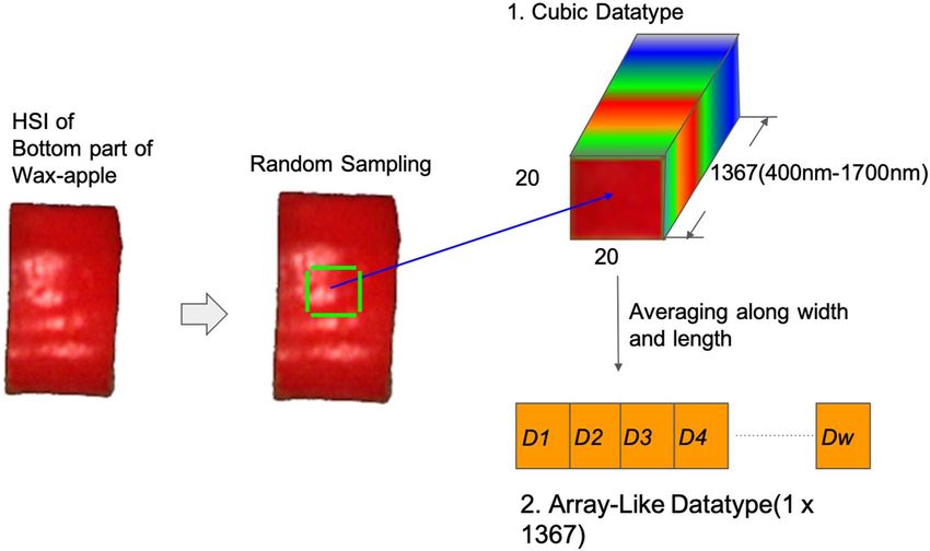
www.nature.com/scientificreports/
Figure 2. The workflow shows that the data augmentation for generating cubic hyperspectral images and the
array-like spectrum averages. The smaller HSIs will be randomly sampled, and the number of the smaller HISs
depends on the size of the wax apple sample. Because this study aims to analyze the spectral features of HSIs, the
spatial features would not be considered in the data augmentation process.
Sugar content Number of SAMPLES
°Brix ∈ [0, 10] (M:8.660, Std:0.813) 254
°Brix ∈ [10, 11] (M:10.448, Std:0.251) 162
°Brix ∈ [11, 12] (M:11.497, Std:0.232) 283
°Brix ∈ [12, 13] (M:12.526, Std:0.272) 218
°Brix ∈ [13, 17] (M:14.027, Std:0.864) 237
Table 1. The table shows the number of samples in each group. The M denotes the mean °Brix, and Std
denotes the standard deviation of samples in each group.
Data visualization with t‑SNE. The t-Distributed Stochastic Neighbor Embedding (t-SNE) is a non-
linear machine learning algorithm proposed by van der Maaten and H inton19. It is a popular manifold learn-
ing algorithm that aims to preserve the feature information when high dimensional data are visualized as low
dimensional data. In t-SNE, the goal is to make the conditional probability [Eq. (2)] of high ( pij ) and low (qij )
dimensional Euclidean distances as close as possible by minimizing the cost function [Eq. (3)], which is the sum
of Kullback–Leibler divergences over all data points.
2
−1
exp(−||xi − xj ||2 /2σi 2 ) 1 +
yi − yj
pij =
2 22
, qij =
2
−1 (2)
k�=l exp(−||xk − xl || )/2σi
1 +
yk − yl
k�=l
pj|i
C=
i
KL(Pi ||Qi ) =
i
pj|i log
qj|i (3)
And because σi is varied for every data point, how σi is selected is here in accordance with a fixed perplexity
Perp(Pi ) = 2H(Pi ) (4)
where H(Pi ) is the Shannon Entropy Pi measured in bits
H(Pi ) = − (pj|i log 2 pj|i )
i
(5)
In this study, data visualization could help to do preliminary analysis. Therefore t-SNE was used to scale the
high dimensional data X (obtained from the preprocessing stage) from d dimension to 2-dimensional data Y ,
Scientific Reports | (2022) 12:2774 | https://doi.org/10.1038/s41598-022-06679-6 4
Vol:.(1234567890)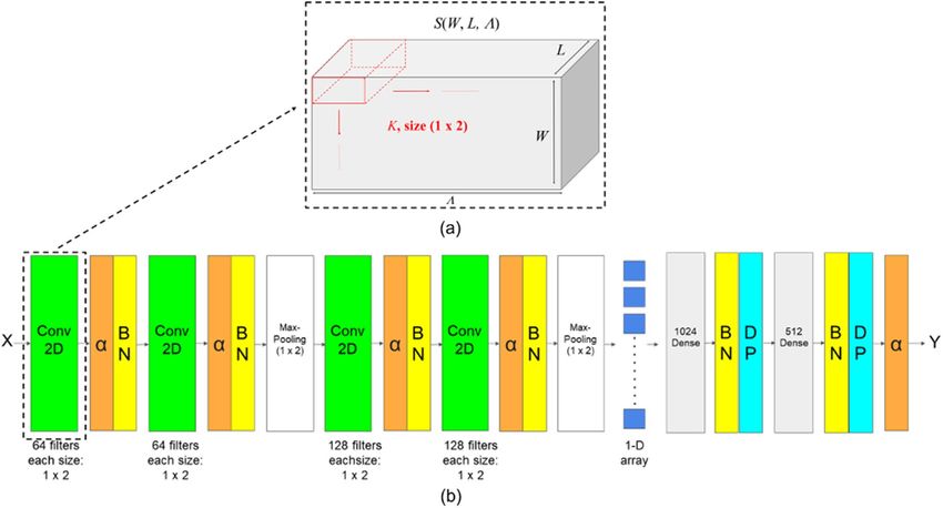
www.nature.com/scientificreports/
Number of samples
Range Size Groups Training Validation Test
°Brix ∈ [0, 10] (M:8.654, Std:0.823) 131 44 43
°Brix ∈ [10, 11] (M:10.448, Std:0.251) 97 33 32
400–1700 nm 20 × 20 × 1367 °Brix ∈ [11, 12] (M:11.487, Std:0.231) 131 44 43
°Brix ∈ [12, 13] (M:12.526, Std:0.272) 131 44 43
°Brix ∈ [13, 17] (M:14.016, Std:0.888) 131 44 43
°Brix ∈ [0, 10] (M:8.654, Std:0.823) 131 44 43
°Brix ∈ [10, 11] (M:10.448, Std:0.251) 97 33 32
400–1000 nm 20 × 20 × 1053 °Brix ∈ [11, 12] (M:11.487, Std:0.231) 131 44 43
°Brix ∈ [12, 13] (M:12.526, Std:0.272) 131 44 43
°Brix ∈ [13, 17] (M:14.016, Std:0.888) 131 44 43
3-D HSIs dataset
°Brix ∈ [0, 10] (M:8.654, Std:0.823) 131 44 43
°Brix ∈ [10, 11] (M:10.448, Std:0.251) 97 33 32
400–700 nm 20 × 20 × 575 °Brix ∈ [11, 12] (M:11.487, Std:0.231) 131 44 43
°Brix ∈ [12, 13] (M:12.526, Std:0.272) 131 44 43
°Brix ∈ [13, 17] (M:14.016, Std:0.888) 131 44 43
°Brix ∈ [0, 10] (M:8.654, Std:0.823) 131 44 43
°Brix ∈ [10, 11] (M:10.448, Std:0.251) 97 33 32
900–1700 nm 20 × 20 × 424 °Brix ∈ [11, 12] (M:11.487, Std:0.231) 131 44 43
°Brix ∈ [12, 13] (M:12.526, Std:0.272) 131 44 43
°Brix ∈ [13, 17] (M:14.016, Std:0.888) 131 44 43
°Brix ∈ [0, 10] (M:8.654, Std:0.823) 131 44 43
°Brix ∈ [10, 11] (M:10.448, Std:0.251) 97 33 32
400–1700 nm 1 × 1367 °Brix ∈ [11, 12] (M:11.487, Std:0.231) 131 44 43
°Brix ∈ [12, 13] (M:12.526, Std:0.272) 131 44 43
°Brix ∈ [13, 17] (M:14.016, Std:0.888) 131 44 43
°Brix ∈ [0, 10] (M:8.654, Std:0.823) 131 44 43
°Brix ∈ [10, 11] (M:10.448, Std:0.251) 97 33 32
400–1000 nm 1 × 1053 °Brix ∈ [11, 12] (M:11.487, Std:0.231) 131 44 43
°Brix ∈ [12, 13] (M:12.526, Std:0.272) 131 44 43
°Brix ∈ [13, 17] (M:14.016, Std:0.888) 131 44 43
1-D spectra data
°Brix ∈ [0, 10] (M:8.654, Std:0.823) 131 44 43
°Brix ∈ [10, 11] (M:10.448, Std:0.251) 97 33 32
400–700 nm 1 × 575 °Brix ∈ [11, 12] (M:11.487, Std:0.231) 131 44 43
°Brix ∈ [12, 13] (M:12.526, Std:0.272) 131 44 43
°Brix ∈ [13, 17] (M:14.016, Std:0.888) 131 44 43
°Brix ∈ [0, 10] (M:8.654, Std:0.823) 131 44 43
°Brix ∈ [10, 11] (M:10.448, Std:0.251) 97 33 32
900–1700 nm 1 × 424 °Brix ∈ [11, 12] (M:11.487, Std:0.231) 131 44 43
°Brix ∈ [12, 13] (M:12.526, Std:0.272) 131 44 43
°Brix ∈ [13, 17] (M:14.016, Std:0.888) 131 44 43
Table 2. The table shows all the information of datasets, each 3-D and 1-D datasets consist of four different
wavelength range spectra datasets where each spectra dataset is composed of five groups of random samples
for °Brix under 10, °Brix 10 to 11, °Brix 11 to 12, °Brix 12 to 13 and °Brix above 13. The M denotes the mean
°Brix, and Std denotes the standard deviation of samples in each group.
where d was the number of data points of whole the bands. The output Y could also be considered as the basis
vectors of X . To obtain the best output Y , Stochastic Gradient Descent with Momentum (SGDM) is applied to
optimize the cost C . The equation of SGDM was defined as
∂C
Y (t) = Y (t−1) − η + α(t) Y (t−1) − Y (t−2) (6)
∂Y
where t is the index of iteration, η is the learning rate and α is the momentum.
First, the max number of the iteration T , learning rate η, momentum α(t), and perplexity Perp were set.
Second, the conditional probability( pij ) of X was calculated using Eq. (2) under a given perplexity value Perp,
then the Principal Component Analysis (PCA) is applied to initialize Y . Third, the conditional probability(qij )
of the initial Y was calculated using Eq. (2), and the cost C was obtained using Eq. (3). Fourth, if not excessing
Scientific Reports | (2022) 12:2774 | https://doi.org/10.1038/s41598-022-06679-6 5
Vol.:(0123456789)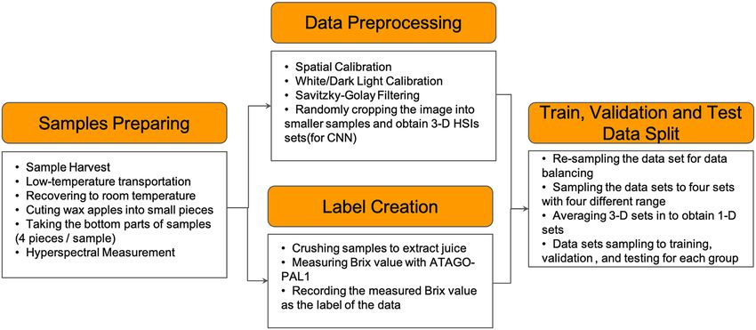
www.nature.com/scientificreports/

                                            Figure 3.  The workflow is designed for preparing experimental datasets. First, the samples are transferred to
                                            the lab under low-temperature transportation. Second, after the samples are recovered to room temperature,
                                            the samples are cut into small pieces for HSIs scanning and juice extracting. Third, the HSIs are obtained by
                                            the imaging system in a dark room. Fourth, the small samples are crushed by a small juicer to extract the juice
                                            to measure the value of sugariness, which is the data label, with a refractometer ATAGO-PAL1. Fifth, the HSIs
                                            are calibrated with spatial calibration and white/dark light calibration, then Savitzky-Golay Filtering is applied
                                            to filter the noise and smooth the waveform. Seventh, each of the HSIs cubes is randomly cropped into smaller
                                            samples for data augmentation. The detail of this step is shown in Fig. 2. Seventh, the datasets are divided into
                                            five groups, including "under °Brix 10", "°Brix 10 to 11", "°Brix 11 to12", "°Brix 12 to13", and "°Brix above 13"
                                            depending on the °Brix. The numbers of data in groups are similar for data balancing. Eighth, the 3-D HSIs
                                            datasets are sampled into four datasets with different band ranges, including 400–1700 nm (each cube with
                                            size 20 × 20 × 1367), 400–1000 nm (each cube with size 20 × 20 × 1053), 400–700 nm (each cube with size
                                            20 × 20 × 575), and 900–1700 nm (each cube with size 20 × 20 × 424). Then, the 3-D datasets are averaged
                                            along their width and length to obtain 1-D datasets. Therefore, there had also four datasets, including 400–
                                            1700 nm (each array with size 1 × 1367), 400–1000 nm (each array with size 1 × 1053), 400–700 nm (each array
                                            with size 1 × 575), and 900–1700 nm (each array with size 1 × 424). Finally, all the datasets are sampled into
                                            "training", "validation", and "test" for modeling.

                                           the max iteration T , the gradient was calculated and Y was updated using Eq. (6). Finally, when the iteration
                                           was done, the final 2-dimensioanl output Y was obtained and visualized on the 2-D plane. The entire workflow
                                           is shown in the Fig. 4.
                                               Furthermore, to visualize the data distribution after the deep learning process to make a contrast, t-SNE
                                           was also used to evaluate the clustering of the outputs before the last regression output layer of proposed deep
                                           learning models. Figure 5. shows the workflow of t-SNE to present learning results. First of all, X was the input
                                           dataset with total N wax apple samples. Each data in X was fed into the proposed deep learning models to obtain
                                           output from the fully-connected layer to the last regression output layer. Second, the N arrays with each size
                                           1 × J , where J denoted as the number of the output of the layer before the last output layer, were composed of
                                           each output obtained by feeding each data in X . Finally, the matrix with size N × J was scaled to matrix N × 2
                                           using t-SNE as same as the process in Fig. 4, which was able to visualize in the 2-D plane.

                                            Hyperspectral and convolutional modeling. Two linear regression techniques and two deep learning
                                            modeling techniques were implemented on our datasets. The linear algorithms Principal Component Regression
                                            (PCR) and Partial Least Square Regression (PLSR) were applied to compare with non-linear deep learning tech-
                                            niques on 1-D spectrum array datasets in this research. Respectively, the proposed deep learning models were
                                            Feedforward Neural Network (FNN) and Convolutional Neural Network (CNN). These two techniques will be
                                            used on 1-D spectra datasets and 3-D HSIs datasets.

                                            Principal component regression and partial least square regression. PCR and PLSR were applied
                                            to our dataset to compare with deep learning methods. PCR is based on the Principal Component Analysis
                                            (PCA) and Multi-Linear Regression (MLR) approach. The main idea of the PCA is to find out the projection
                                            vector v* that can maximize the variation of the projected data and can be denoted as Eq. (7), where the M is the
                                            covariance matrix, and Rd is the domain of data.

                                                                                           v ∗ = argmax v T Cv                                             (7)
                                                                                                    v∈Rd

                                               Each vector that is found by Eq. (7) will be treated as the principal components (PCs), the first component
                                            will dominate the most significant percentage of data variance, and the following components will have the

          Scientific Reports |   (2022) 12:2774 |                https://doi.org/10.1038/s41598-022-06679-6                                                  6

Vol:.(1234567890)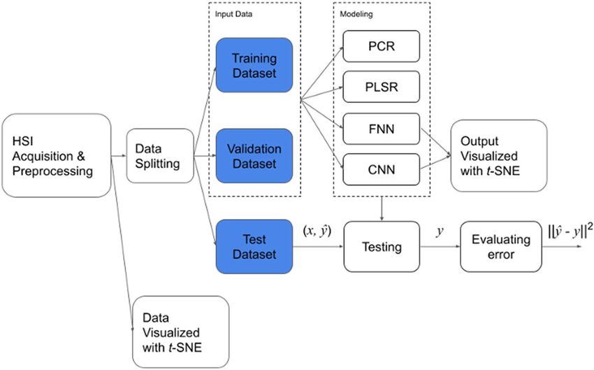
www.nature.com/scientificreports/

                                 Figure 4.  The workflow shows how this study implements t-SNE. The high dimensional array with spectra data
                                 ( X ) corresponding to wavelength is averaged from 3-D HSIs datasets along width and length. After setting the
                                 max number of the iteration T , learning rate η, momentum α(t), and perplexity Perp, the conditional probability
                                 ( pij) of X is calculated under given Perp, then the Principal Component Analysis (PCA) is applied to initialize
                                 Y . To minimize cost C , the Stochastic Gradient Descent with Momentum (SGDM) is applied. When the
                                 optimization process is done, the final output Y is obtained and visualized on the 2-D plane.

                                  Figure 5.  The workflow shows how t-SNE evaluates the learning results. First, the matrix with the size is
                                  obtained by feeding the dataset X to proposed deep learning models and collecting the layer’s outputs before the
                                  last regression output layer. Then the matrix is scaled to N data points to visualize the t-SNE result. The process
                                  of t-SNE is as same as the process in Fig. 4.

                                  decreasing data variance for the whole signal, the PCs could be found by the singular value decomposition. All of
                                  them are linear combinations of the initial signal but not unrelated to each other. This method has the advantage
                                  of decreasing the disturbance from noise or small signals, and it is often utilized with a multidimensional reduc-
                                  tion that retains the essential components before the following procedure. This method can eliminate the multi-
                                  collinearity because the PCs are uncorrelated. However, the PCR has the drawback that the PCs are obtained
                                  through only variables themselves. It cannot ensure that the variables correlate with the observation data, which
                                  often makes lower precision outcomes from the fitting model. Consequently, it is trendy that combining with
                                  other discriminant methods for target detecting or classifying.
                                      PLSR20 was proposed to overcome the drawback of PCR; PLSR extracts the dependent variables by confirming
                                  their predictive abilities. These orthogonal factors, which are also known as latent variables (LVs), are obtained
                                  according to the correlation with the predicting variable. The general basic model of PLSR can be denoted as
                                  Eqs. (8) and (9), where X is the matrix of predictors, Y is a matrix of response, T and U are the projection of X
                                  and Y , P and Q are coefficient matrices, E and F are the error terms. The main idea of the PLSR is to look for the

Scientific Reports |   (2022) 12:2774 |                https://doi.org/10.1038/s41598-022-06679-6                                                   7

                                                                                                                                               Vol.:(0123456789)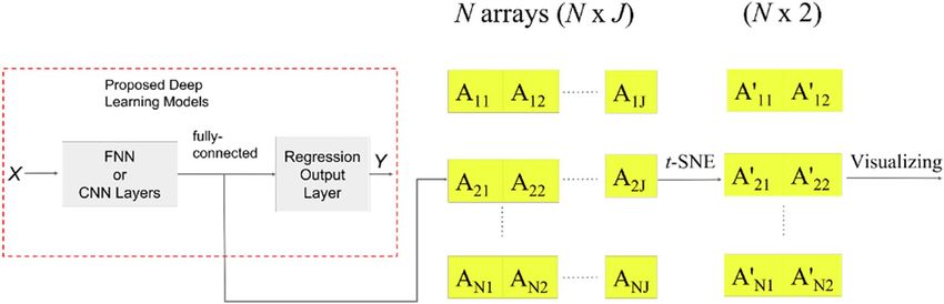
www.nature.com/scientificreports/
Figure 6. The figure shows the architecture of the proposed feedforward neural network for sugariness. Input
is a 1-D spectra data with size for the number of bands. Hidden layers contain one layer with 2048 neurons and
another layer with 512 neurons, each layer connected with a ReLU activation function (α), batch normalization
layer (BN), and dropout layer (DP). The final output Y is the sugariness prediction result of the model.
proper projection that has the maximum correlation shown in Eq. (10). Different from the PCA, which extracts
the PCs with a high covariance variable, the PLSR is more feasible in the condition of multi-collinearity between
the variables. Thus, the number of LVs is usually less than PCs in PCR regression.
X = TP T + E (8)
Y = UQT + F (9)
t, u = argmax Cov(T, U) (10)
T,U
Feedforward neural network. The concept of the feedforward neural network (FNN) model was intro-
duced by Rosenblatt in 1 95821. In this work, FNN was applied to analyze N × W data where N denotes the
number of samples and W denotes the number of bands. The proposed FNN model, illustrated in Fig. 6, was
designed with the input layer consisting of individual hyperspectral bands of input data, hidden layers contain-
ing 2048 and 512 neurons with the batch normalization layer and dropout layer to prevent overfitting in model
training, and one neuron for the output layer, each layer activated with the Rectified Linear Unit, ReLU(α),
activation function. In our study, there were still some outliers in our dataset. Therefore, the Root Mean Squared
Log Error (RMSLE) was used to evaluate training errors. Referring to Root Mean Squared Error (RMSE), Root
Mean Squared Logarithmic Error (RMSLE) is yielded by
1
n 2
(11)
′
RMSLE = (log(Y i + 1) − log(Yi + 1))
n i
′
where Y is the predicted value, and Y is the target. This measure shows the ability to nullify the effects of outliers
by reducing the difference between and with the natural logarithm.
Convolutional neural networks. Convolutional Neural Network (CNN) was also one of the approaches
applied to our dataset. LeCun proposed the modern CNN architecture in 1 99822. Its strong ability to extract
spatial features makes it achieve state-of-the-art performance in computer vision tasks. However, in this study,
instead of extracting spatial features, the 2-D CNN model was used to extract spectral features from 3-D HSIs.
The proposed 2-D convolutional layer to extract spectral features of HSIs with one kernel is shown in Fig. 7a.
To extract spectral features, the cube with size (W, L, �) would be rotated in the convolution process, where W
denotes the width of HSIs with constant value 20, L denotes the length of HSIs with constant value 20, and
denotes the number of bands of a hyperspectral image. The 2-D convolutional layer was designed to conduct
the convolution along the surface (W, �) and consider the length of HSIs L as the channels and apply the kernel
to all the channels. Therefore, a 2-D feature map represented as spectral features would be obtained after the
convolution of HSIs and a single kernel. The value of the 2-D feature map at the position (ω, l, ) denoted as G
(ω, l, ) is given by
Scientific Reports | (2022) 12:2774 | https://doi.org/10.1038/s41598-022-06679-6 8
Vol:.(1234567890)
www.nature.com/scientificreports/
Figure 7. Figure (a) presents the proposed 2-D convolutional layer for extracting spectral features of the HSIs
H with size (W, L, �). Figure (b) shows the architecture of the proposed convolutional network for sugariness
prediction. Input X is a 3-D HSIs cube sample, and the network contains four convolutional layers with a ReLU
activation function. Batch normalization (BN) layers and Dropout (DP) layers are used to prevent overfitting. In
the last Maxpooling layer, its output is a 1-D array obtained by calculating the maximum from each 1 × 2 patch
of the feature map then flattening. The 1-D array was then fed to fully connected layers with two dense layers
with BN and DP following to regress the sugariness prediction result Y.
ω −1 k
k −1
′ ′
′ ′
G(ω, l, ) = K ω , S ω − ω , l, − (12)
′ ′
ω =0 =0
′
where ω′ and are the index of the kernel, kω and k are the width and length of the kernel, ω , l , and are the
position of HSIs, S is the HSIs, and K is a kernel in the proposed 2-D convolutional layer. Optimizing convo-
lutional network was used to find the optimal kernel parameters which provide high impulse response to local
spectral features. The calculated response was feasible to apply Maxpooling to preserve the spectral features with
high response. By applying the backpropagation algorithm, the kernel parameters were updated to reduce the
regression error for the downstream task. Based on this solution, the spectral features which map to the features
of sugariness could be found.
The entire architecture of the model is shown in Fig. 7b. A model was designed to extract spectral features
from the HSIs, which had four convolutional layers with filter size 1 × 2(kω = 1, and k = 2) and two Maxpooling
layers with size 1 × 2 and fully connected layers with 1 × 1 dense layer for output, all the convolutional layers
with Batch Normalization (BN) and Rectified Linear Unit (ReLU) as the non-linear activation function. As
mentioned earlier, the convolutional layer was designed to extract spectral features, and the Maxpooling layers
were also designed to extract spectral features.
′ Assume
after conducting the convolution, normalization, and
′ ′
activation, the cubic feature map with size W , L , was
obtained. Then the Maxpooling layers would select
′ ′
the maximum from each 1 × 2 patch on the space W , in order to preserve the spectral features. Therefore,
′ ′ ′
the size of the feature map after pooling would be W2 , L , 2 . After extracting features, the output feature map
obtained from the last Maxpooling layer is flattened to a 1-D array and fed into fully connected layers. Finally,
the final activation layer was also a ReLU function. It gave a °Brix value of the wax apple sample, and the error
is evaluated with Root Mean Squared Logarithmic Error (RMSLE) in Eq. (10).
Ethical approval. The collection of the cultivated plants of this study complied with the relevant institu-
tional, national, and international guidelines and legislation. The farmers permitted the transaction of plants in
studying usage. If request, the datasets of HSIs of wax apples will be available.
Scientific Reports | (2022) 12:2774 | https://doi.org/10.1038/s41598-022-06679-6 9
Vol.:(0123456789)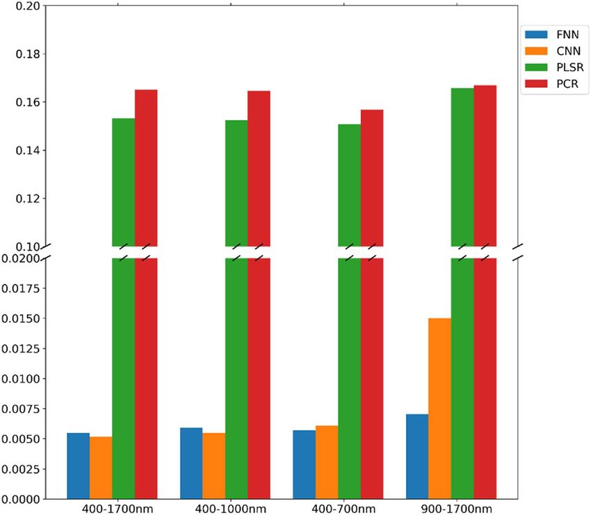
www.nature.com/scientificreports/
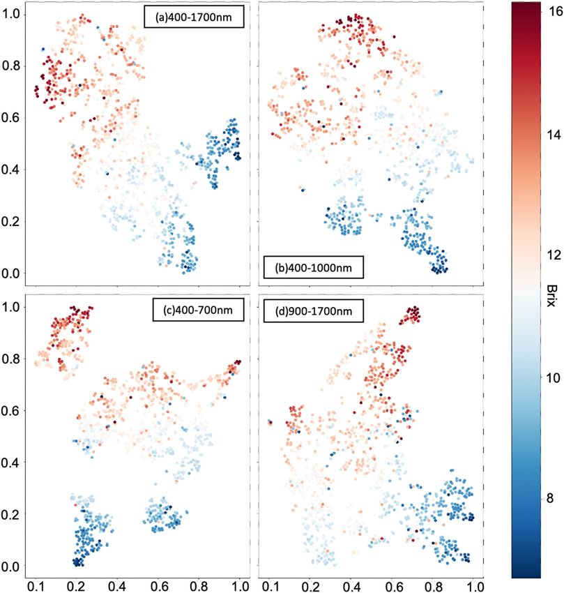
Figure 8. The figure shows the results of t-SNE on the four datasets, (a–d) are the datasets of wavelength range
400–1700 nm, 400–1000 nm, 400–700 nm, and 900–1700 nm, the color bar in the right side denoted the °Brix
value of each data point. All the t-SNE results are obtained with the perplexity value 20, the 30,000 iteration
times, and the learning rate 1000. The horizontal and vertical coordinates are the coordinate of data points
obtained from dimension reduction using t-SNE.
Results
Evaluation by data visualization. In the experiments, t-SNE was applied to reduce the dimensionality
of HSIs and visualize the distribution of the datasets, the workflow of t-SNE shown in Fig. 4. The dataset X used
to make dimension reduction were the array datasets averaged from 3-D HSIs, because it would be time-con-
suming, and the results were not too much different with 3-D HSIs. The entire dataset contained 932 reflectance
spectral data arrays for different bands. Before starting the t-SNE algorithm in the experiment, the Principal
Component Analysis (PCA) was used to initialize the value for dimension reduction results Y . Then the t-SNE
models were trained with the perplexity value 20, the 30,000 iteration times, and the learning rate 1000 with
SGDM. Figure 8 shows the visualization results of four different datasets.
Scientific Reports | (2022) 12:2774 | https://doi.org/10.1038/s41598-022-06679-6 10
Vol:.(1234567890)www.nature.com/scientificreports/
Figure 9. The bar chart shows the validation loss (RMSLE) of each proposed model. In the optimization
process, the weights with the smallest validation loss are recorded as the best sets. This validation error
presented in the chart indicates that FNN and CNN would have superior performance compared with PCR and
PLSR on the datasets.
Figure 8a–c show the t-SNE results of datasets with wavelength 400–1700 nm, 400–1000 nm, and
900–1700 nm, although the data points of sugariness above 13°Brix and under 10°Brix seem to be clustered, the
clusters of data points with sugar content between 13°Brix and 10°Brix seem to be ambiguous. On the other hand,
the clusters of t-SNE results shown in Fig. 8d are much more ambiguous than the different datasets. Therefore,
it would indicate that the spectra data of wavelength 400–1000 nm were more significant than the spectra data
of wavelength 900–1700 nm to regress the sugariness value. This t-SNE result reveals that the spectra data of
visible spectroscopy (VIS) bands could contain more significant features toward predicting sugariness than the
near-infrared (NIR) spectroscopy bands.
Evaluation over different models. The weights and kernels in FNN and CNN models were initialized
with Glorot initialization23 and regularized with L2 regularization24 with regularization parameter 3 × 10⁻⁵
while training. Adam optimizer25 was used with mini-batch 128 and 3000 epochs for all the models to optimize
the weights of each layer of FNN models and kernels of CNN models. Learning rate decay method applied in
the experiments for optimizing models, the initial learning rate value for first epoch was 1 × 10⁻³, and an expo-
nential decay lr t = lr t−1 ∗ e(−k∗t) (lr denotes as the learning rate, t denotes as the epoch number, k denoted as a
constant of 1 × 10⁻⁴) was applied for following epochs.
The bar chart Fig. 9 shows the RMSLE of each method on the validation set. The trained weights were cho-
sen at the step with the smallest validation loss in the optimization process for testing each of the deep learning
models. The minimum of the validation loss of each FNN model for 400–1700 nm, 400–1000 nm, 400–700 nm,
and 900–1700 nm were 0.005463 at step 2734, 0.005917 at step 2736, 0.005707 at step 2540, and 0.007042 at step
2980. The model for 400–1700 nm had the lowest loss, and the model for 900–1700 nm had the highest loss, so
it was expectable that the FNN model for 400–1700 nm would have better performance on the test dataset than
the other FNN models. There were also four models for CNN. The minimum of validation loss (RMSLE) of the
400–1700 nm model was 0.005165 at step 2844, 0.005478 at step 2732 for the model of 400–1000 nm, 0.006077 at
step 2092 for the model of 400-700 nm, and 0.015015 at the step 2994 for the model of 900–1700 nm. As same as
the results of FN models, the CNN model for 400–1700 nm had the lowest loss, and the model for 900–1700 nm
had the highest loss. Comparing the results of FN with the results of CNN models, the CNN models would have
better performance than FNN models. The deep learning modeling was implemented using the Keras26 and
Tensorflow backend27 on an NVIDIA RTX 3090 GPU.
PCR and PLSR were used to make a comparison with deep learning methods on the same training data-
sets. The PCR result showed that the validation loss (RMSLE) on four validation datasets was 0.165022 for the
Scientific Reports | (2022) 12:2774 | https://doi.org/10.1038/s41598-022-06679-6 11
Vol.:(0123456789)www.nature.com/scientificreports/
Averaged sugar content error in each interval(± °Brix)
0–10 10–11 11–12 12–13 Above 13 All
Method Band range 43 samples 32 samples 43 samples 43 samples 43 samples 162 samples
400–1700 nm 2.727 1.061 0.218 1.103 2.430 1.532
400–1000 nm 2.678 1.051 0.233 1.107 2.441 1.526
PCR
400–700 nm 2.504 0.942 0.339 1.018 2.287 1.444
900–1700 nm 2.797 1.063 0.180 1.080 2.394 1.526
400–1700 nm 2.449 0.927 0.360 0.979 2.119 1.391
400–1000 nm 2.410 0.954 0.371 0.965 2.098 1.382
PLSR
400–700 nm 2.405 0.958 0.375 0.218 2.369 1.379
900–1700 nm 2.821 1.049 0.218 1.100 2.369 1.536
400–1700 nm 0.642 0.646 0.511 0.564 0.637 0.597
400–1000 nm 0.625 0.633 0.437 0.474 0.889 0.610
FNN
400–700 nm 0.732 0.693 0.355 0.463 0.892 0.623
900–1700 nm 0.710 0.656 0.576 0.701 1.032 0.732
400–1700 nm 0.609 0.474 0.412 0.421 0.660 0.552
400–1000 nm 0.627 0.487 0.451 0.516 0.965 0.616
CNN
400–700 nm 0.551 0.408 0.462 0.555 0.914 0.587
900–1700 nm 1.519 0.725 0.496 0.480 1.543 0.965
Table 3. The table shows all the test errors in different band ranges and °Brix value intervals. The average test
results of FNN and CNN indicate that the models have a decent complexity for datasets. On the other hand,
PCR and PLSR would have underfitting problems on the datasets. The better average sugar content for all the
samples is shown in bold. The marked results have the error below ± 0.6°Brix.
400–1700 nm model, 0.164529 for the 400–1000 nm model, 0.156733 for the 400–700 nm model, and 0.166839
for the 900–1700 nm model. On the other hand, validation losses of PLSR were 0.153204, 0.152438, 0.150596,
and 0.16576 on four different datasets. These results indicate that the PLSR method would perform better than
PCR on the collected datasets, and deep learning methods would be much better than PCR and PLSR.
The test results of °Brix of PCR, PLSR, FNN, and CNN models in each interval are shown in Table 3. First
of all, although PCR and PLSR showed their good capability in predicting sugar content in °Brix 11 to 12, the
test errors in other °Brix intervals and averaged test errors were not competitive with errors of FNN and CNN
models. This phenomenon indicated that the PCR and PLSR could have an overfitting problem on this dataset
and improperly detect sugar content of wax apple. The FNN models had the average error with ± 0.597°Brix on
the dataset 400–1700 nm, 400–1000 nm with ± 0.610°Brix, 400–700 nm with ± 0.623°Brix, and 900–1700 nm
with ± 0.739°Brix. The test results showed that FNN models trained using the dataset of wavelength range
400–1700 nm had adequate performance, and wavelength range 900–1700 nm would not correlate with sugar
content prediction using FNN. The test results of CNN models were also similar to the test results of FNN
models. The test error was ± 0.552°Brix on the dataset of wavelength 400–1700 nm, ± 0.616°Brix on the dataset
of wavelength 400–1000 nm, ± 0.587°Brix on the dataset of wavelength 400–700 nm, and ± 0.7396°Brix on a
dataset of wavelength 900–1700 nm. The test results of CNN models were superior to FNN models. Both FNN
and CNN results showed that spectra data corresponding to 400–1700 nm, 400–1000 nm, and 400–700 had
better correlation than data corresponding to 900–1700 nm. This conclusion indicated that VIS bands with
wavelength 400–700 nm might be more correlative to predict sugar content than NIR bands with wavelength
900–1700 nm. However, the combination of VIS bands and NIR bands would help the FNN and CNN models
get a better sugariness prediction result rather than only with VIS bands or NIR bands. On the other hand, the
minimal error of PCR and PLSR were ± 1.444°Brix and ± 1.379°Brix on the dataset of wavelength 400–700 nm, but
both of them had their best (± 0.180°Brix and ± 0.218°Brix) in °Brix interval 11–12 on 900–1700 nm. Therefore,
PCR and PLSR were more severe with overfitting problems on predicting sugar content using spectra data with
wavelength range 900–1700 nm than the other band range. The averaged test error of each learning method
on different band ranges was presented in Fig. 10. The outcomes of test data indicated that the deep learning
methods FNN and CNN were more remarkable than PCR and PLSR on predicting sugariness. These results were
also reflected in validation results.
Evaluation of the learning results by visualizing the outputs before the last layer. Visualization
was also a decent way to evaluate the proposed deep learning models. Therefore, t-SNE was applied to visualize
the outputs of the layer before the last regression output layer. As same as the previous implementation of t-SNE,
the PCA was used as the initial value for dimension reduction results, the perplexity value was set 20, the 30,000
iteration times, and the learning rate 1000 were used in this implementation for SGDM. The workflow is shown
in Fig. 5. Figures 11 and 12 show the final visualization results of MLP and CNN models corresponding to four
different wavelength ranges.
For MLP models, the output size of the layer before the last output layer was 512. Therefore, the output was an
array with size 1 × 512. Then all the outputs from feeding all the datasets ( N × 512) were collected as the input
Scientific Reports | (2022) 12:2774 | https://doi.org/10.1038/s41598-022-06679-6 12
Vol:.(1234567890)www.nature.com/scientificreports/
Figure 10. The bar chart shows that the test result of each model. The test results of FNN and CNN have more
minor errors than PCR and PLSR. It indicates that the performance of non-linear deep learning models is better
than linear models on the datasets.
data X for t-SNE, and scaled to it’s basis vectors Y which were visualized in the Fig. 11. In the Fig. 11a–c show
the final evaluation results corresponding to wavelength range 400–1700 nm, 400–1000 nm, and 400–700 nm
and although there are still some vague clusters, each of the results presents the proper color gradation generally
from deep red to deep blue with respect to high sugar content value to low sugar content value, which represents
the acceptable learning ability of MLP models on those datasets. Although the visualization results were better
than the t-SNE results of the original data, ambiguous clusters are still contained in Fig. 11d. Therefore, this result
elaborates that wavelength 900–1700 nm spectra data would not be advantageous for sugar content prediction.
On the other hand, Fig. 12a–d visualize the t-SNE results on the outputs of the layer before the last output
layer of CNN models corresponding to the wavelength range 400–1700 nm, 400–1000 nm, 400–700 nm, and
900–1700 nm. According to the CNN architecture shown in Fig. 7b, each of the data points in Fig. 12 was also
obtained by scaling output from 1 × 512 to the array with size 1 × 2 using t-SNE. The t-SNE visualization results
gave the fine gradational effect shown in Fig. 12a–d. However, more outliers appeared in clusters of t-SNE results
in Fig. 12d. These results showed that the CNN models could learn features toward the sugar content prediction
by showing better clustering results on outputs before the last regression output layer than the ones on original
data.
Conclusions and discussion
This study aims to predict the sugariness of Syzygium samarangense from hyperspectral images using deep learn-
ing methods. The HSIs were collected from the bottom part of the wax apple and adequately processed to 1-D
spectra datasets and 3-D HSIs datasets. The spectra data were adequately sampled and divided into 400–1700 nm,
400–1000 nm, 400–700 nm, and 900–1700 nm to facilitate learning from the corrected datasets, then t-SNE
was used to evaluate the performance of the spectral band. In the modeling stage, the FNN and CNN models
were designed for analyzing the HSIs datasets. For comparing with deep learning methods, PCR and PLSR were
used on the same datasets. The best results of FNN and CNN were 0.552 and 0.597 (± °Brix) on datasets with
400–1700 nm, relatively, PCR and PLSR had their best result on datasets with 400–700 nm, which were 1.379 and
1.444 (± °Brix). In this study, FNN and CNN models outperformed PCR and PLSR models. Otherwise, all their
well-performed results were obtained with the spectra data with a combination of VIS bands and NIR bands, and
the results with only using NIR bands (900–1700 nm) were not that acceptable. Therefore, this study revealed
that VIS bands would be more critical in predicting sugar content, but it would be better with the combination
of VIS bands and NIR bands. This result showed the potential performance on acquiring sugar content of wax
apple with spectra data corresponding to VIS bands and NIR bands using a deep learning model. However, only
the NIR bands would not be recommended. Moreover, the improved t-SNE results on the final regression outputs
before the last layer of proposed deep learning models show that FNN and CNN models would adequately learn
how to predict sugariness from the HSIs datasets.
Compared with the previous s tudy10, this paper provided the average error and the error in each °Brix interval
within one °Brix. Although their works had good prediction results with total SEV = 0.381 and 0.426°Brix for
ICA and PLSR using only NIR bands, this study indicated that the error would be significantly different within
different sugar content intervals. Therefore, this study which provided errors of different sugar content intervals,
would be more detailed than theirs.
It will be significant to select proper bands for fabricating a portable device to detect sugariness in future work.
The light source with VIS bands and the CNN model would be a good start for constructing a mobile device
because the light source with VIS bands is more easily available than NIR bands. Moreover, although without
NIR bands, the combination of the CNN model with VIS bands shows adequate performance on prediction
sugariness of wax apple in this study with the minor error in interval 0 to 10°Brix and 10 to 11°Brix are ± 0.551
and ± 0.408. These results indicate that the CNN model using VIS spectra data would have the capability to
Scientific Reports | (2022) 12:2774 | https://doi.org/10.1038/s41598-022-06679-6 13
Vol.:(0123456789)www.nature.com/scientificreports/
Figure 11. The figure shows the result of t-SNE on the outputs obtained by feeding the four datasets to FNN
models, (a–d) are the datasets of wavelength range 400–1700 nm, 400–1000 nm, 400–700 nm, and 900–
1700 nm. The color bar on the right side is denoted as the °Brix of each data point. Compared to t-SNE results
on original datasets, figures (a–c) generally show a fine color gradation from deep red to deep blue. Relatively
figure (d) contains more vague clusters than others. The horizontal and vertical coordinates are the coordinate of
the basis vectors, which are obtained from dimension reduction using t-SNE.
predict if sugariness is below 10°Brix or not. This would be similar to the human’s eyes because when the wax
apples get ripe, the wax apples gain more sugar and become more scarlet than before. Therefore, the human’s eyes
could roughly detect the sugar contents by the color of the wax apples. However, this study also indicates that if
both the visible and invisible spectral features are considered, it would better predict the sugariness of wax apples.
Scientific Reports | (2022) 12:2774 | https://doi.org/10.1038/s41598-022-06679-6 14
Vol:.(1234567890)www.nature.com/scientificreports/
Figure 12. The figure shows the t-SNE results on the outputs obtained by feeding the four datasets to CNN
models are visualized in (a–d) corresponding to wavelength range 400–1700 nm, 400–1000 nm, 400–700 nm,
and 900–1700 nm. The color bar on the right side is represented as the °Brix of each data point. Compared to
t-SNE results on original datasets, figures (a–d) generally show the better color gradation from deep red to deep
blue. Although there are some outliers contained in clusters in figure (d), the t-SNE visualization results in the
figure (a–d) are much better than ones in Fig. 8a–d. The horizontal and vertical coordinates are referred to as
the coordinate of basis vectors obtained from dimension reduction using t-SNE.
Received: 27 June 2021; Accepted: 11 January 2022
References
1. Taghizadeh, M., Gowen, A. A. & O’Donnell, C. P. Comparison of hyperspectral imaging with conventional RGB imaging for quality
evaluation of Agaricus bisporus mushrooms. Biosyst. Eng. 108(2), 191–194. https://doi.org/10.1016/j.biosystemseng.2010.10.005
(2011).
Scientific Reports | (2022) 12:2774 | https://doi.org/10.1038/s41598-022-06679-6 15
Vol.:(0123456789)www.nature.com/scientificreports/
2. Bioucas-Dias, J. M. et al. Hyperspectral remote sensing data analysis and future challenges. IEEE Geosci. Remote Sens. Mag. 1(2),
6–36. https://doi.org/10.1109/MGRS.2013.2244672 (2013).
3. Akhtar, N. & Mian, A. Nonparametric coupled Bayesian dictionary and classifier learning for hyperspectral classification. IEEE
Trans. Neural Netw. Learn. Syst. 29(9), 4038–4050. https://doi.org/10.1109/TNNLS.2017.2742528 (2017).
4. Zhong, P. & Wang, R. Jointly learning the hybrid CRF and MLR model for simultaneous denoising and classification of hyper-
spectral imagery. IEEE Trans. Neural Netw. Learn. Syst. 25(7), 1319–1334. https://doi.org/10.1109/TNNLS.2013.2293061 (2014).
5. Peiris, K. H. S., Dull, G. G., Leffler, R. G. & Kays, S. J. Near-infrared spectrometric method for non-destructive determination of
soluble solids content of peaches. J. Am. Soc. Hortic. Sci. 123(5), 898–905. https://doi.org/10.21273/JASHS.123.5.898 (1998).
6. Mendoza, F., Lu, R., Ariana, D., Cen, H. & Bailey, B. Integrated spectral and image analysis of hyperspectral scattering data for
prediction of apple fruit firmness and soluble solids content. Postharvest Biol. Technol. 62(2), 149–160. https://doi.org/10.1016/j.
postharvbio.2011.05.009 (2011).
7. Park, B., Abbott, J. A., Lee, K. J., Choi, C. H. & Choi, K. H. Near-infrared diffuse reflectance for quantitative and qualitative measure-
ment of soluble solids and firmness of Delicious and Gala apples. Trans. ASAE 46(6), 1721. https://doi.org/10.13031/2013.15628
(2003).
8. Liang, P. S. et al. Non-destructive detection of zebra chip disease in potatoes using near-infrared spectroscopy. Biosyst. Eng. 166,
161–169. https://doi.org/10.1016/j.biosystemseng.2017.11.019 (2018).
9. Kemps, B., Leon, L., Best, S., De Baerdemaeker, J. & De Ketelaere, B. Assessment of the quality parameters in grapes using VIS/
NIR spectroscopy. Biosys. Eng. 105(4), 507–513. https://doi.org/10.1016/j.biosystemseng.2010.02.002 (2010).
10. Chuang, Y. K. et al. Integration of independent component analysis with near infrared spectroscopy for rapid quantification of
sugar content in wax jambu (Syzygium samarangense Merrill & Perry). J. Food Drug. Anal. 20(855), e64. https://doi.org/10.6227/
jfda.2012200415 (2012).
11. Viegas, T. R., Mata, A. L., Duarte, M. M. & Lima, K. M. Determination of quality attributes in wax jambu fruit using NIRS and
PLS. Food Chem. 190, 1–4. https://doi.org/10.1016/j.foodchem.2015.05.063 (2016).
12. Gao, Z. et al. Real-time hyperspectral imaging for the in-field estimation of strawberry ripeness with deep learning. Artif. Intell.
Agric. 4, 31–38. https://doi.org/10.1016/j.aiia.2020.04.003 (2020).
13. Itakura, K., Saito, Y., Suzuki, T., Kondo, N. & Hosoi, F. Estimation of citrus maturity with fluorescence spectroscopy using deep
learning. Horticulturae 5(1), 2. https://doi.org/10.3390/horticulturae5010002 (2019).
14. Tu, S. et al. Passion fruit detection and counting based on multiple scale faster R-CNN using RGB-D images. Precision Agric. 21(5),
1072–1091. https://doi.org/10.1007/s11119-020-09709-3 (2020).
15. Fajardo, M. & Whelan, B. M. Within-farm wheat yield forecasting incorporating off-farm information. Precision Agric. 22, 569–585.
https://doi.org/10.1007/s11119-020-09779-3 (2021).
16. Marani, R., Milella, A., Petitti, A. & Reina, G. Deep neural networks for grape bunch segmentation in natural images from a
consumer-grade camera. Precision Agric. 22(2), 387–413. https://doi.org/10.1007/s11119-020-09736-0 (2021).
17. Li, Y. S. et al. Development and verification of the coaxial heterogeneous hyperspectral system for the Wax Apple tree. in Interna-
tional Instrumentation and Measurement Technology Conference, 1–5. https://doi.org/10.1109/I2MTC.2019.8826836 (2019).
18. Savitzky, A. & Golay, M. J. E. Smoothing and differentiation of data by simplified least squares procedures. Anal. Chem. 36(8),
1627–1639. https://doi.org/10.1021/ac60214a047 (1964).
19. Van der Maaten, L. & Hinton, G. Visualizing data using t-SNE. J. Mach. Learn. Res. 9(11), 1–10 (2008).
20. Wold, S., Sjöström, M. & Eriksson, L. PLS-regression: A basic tool of chemometrics. Chemom. Intell. Lab. Syst. 58(2), 109–130.
https://doi.org/10.1016/S0169-7439(01)00155-1 (2001).
21. Rosenblatt, F. The perceptron: A probabilistic model for information storage and organization in the brain. Psychol. Rev. 65,
386–408. https://doi.org/10.1037/h0042519 (1958).
22. LeCun, Y., Bottou, L., Bengio, Y. & Haffner, P. Gradient-based learning applied to document recognition. Proc. IEEE 86(11),
2278–2324. https://doi.org/10.1109/5.726791 (1998).
23. Glorot, X., & Bengio, Y. Understanding the difficulty of training deep feedforward neural networks. In Proceeding of International
Conference on Artificial Intelligence and Statistics, 249–256. http://proceedings.mlr.press/v9/glorot10a.html (2010).
24. Cortes, C., Mohri, M., & Rostamizadeh, A. L2 Regularization for Learning Kernels. https://arxiv.org/abs/1205.2653 (2012).
25. Kingma, D. P., & Ba, J. Adam: A Method for Stochastic Optimization. https://arxiv.org/abs/1412.6980 (2014).
26. Gulli, A., & Pal, S. Deep learning with Keras. Packt Publishing Ltd. https://keras.io/ (2017).
27. TensorFlow. API TensorFlow Core v2.3.0: Python. https://www.tensorflow.org/api_docs/python/tf. (2020). Accessed 1 Mar 2020.
Acknowledgements
This work is supported by the Council of Agriculture, Taiwan under Project (COA 108AS-13.2.11-ST-a6, COA
107AS-14.2.11-ST-a3) and by the Ministry of Science and Technology, Taiwan under Project (MOST 110-2321-
B-A49-001, MOST 109-2321-B-009-008-s, MOST 108-2321-B-009-001, MOST 108-2221-E-009-125, MOST
107-2321-B-009-002, MOST 107-2622-E-009-015-CC2, MOST 107-2221-E-009-155), and National Yang Ming
Chiao Tung University.
Author contributions
C.J.C. did the experiments and prepared the manuscript, including figures and tables. Y.J.Y. provided sugges-
tions in experiments and revisions of the manuscript. C.C.H. helped with samples and knowledge of wax apple.
J.T.C., C.T.C., and J.W.J. provided suggestions about deep learning. T.C.C., S.G.L., R.S.S., and M.O.-Y. provided
suggestions in revisions of the manuscript. All authors read and approve the manuscript.
Competing interests
The authors declare no competing interests.
Additional information
Correspondence and requests for materials should be addressed to M.O.-Y.
Reprints and permissions information is available at www.nature.com/reprints.
Publisher’s note Springer Nature remains neutral with regard to jurisdictional claims in published maps and
institutional affiliations.
Scientific Reports | (2022) 12:2774 | https://doi.org/10.1038/s41598-022-06679-6 16
Vol:.(1234567890)You can also read