A New Derivation of Exact Solutions for Incompressible Magnetohydrodynamic Plasma Turbulence
←
→
Page content transcription
If your browser does not render page correctly, please read the page content below

Copyright © 2021 by American Scientific Publishers                                               Journal of Nanofluids
                      All rights reserved.                                                                           Vol. 10, pp. 98–105, 2021
                      Printed in the United States of America                                                         (www.aspbs.com/jon)

          A New Derivation of Exact Solutions for
          Incompressible Magnetohydrodynamic
          Plasma Turbulence
          Adel M. Morad1, 2, ∗ , S. M. A. Maize3 , A. A. Nowaya3 , and Y. S. Rammah3
          1
            Department of Mathematics and Computer Science, Menoufia University, Shebin-Elkoom, 32511 Egypt
          2
            Department of Computational Mathematics and Mathematical Physics, Institute of Mathematics,
          Mechanics and Computer Science, Southern Federal University, Rostov on Don, 344090 Russia
          3
            Physics Department, Faculty of Science, Menoufia University, Shebin Elkom, 32511 Egypt

          The objective of this paper is to study the propagation of nonlinear, quasi-parallel, magnetohydrodynamic waves
          of small-amplitude in a cold Hall plasma of constant density. Magnetohydrodynamic equations, along with the
          cold plasma were expanded using the reductive perturbation method, which leads to a nonlinear partial differ-
          ential equation that complies with a modified form of the derivative nonlinear evolution Schrödinger equation.
          Exact solutions of the turbulent magnetohydrodynamic model in plasma were formulated for the physical quan-
          tities that describe the problem completely by using the complex ansatz method. In addition, the complete
ARTICLE

          set of equations was used taking into account the magnetic field, which can be considered to be constant in
          the x-direction to create stable vortex waves. Vortex solutions of the modified nonlinear Schrödinger equation
          (MNLS) were compared with the solutions of incompressible magnetohydrodynamic equations. The obtained
                                          IP: 192.168.39.151
          equations differ from the standard    NLS equationOn:by Wed,   13 Oct 2021
                                                                  one additional   term10:20:36
                                                                                         that describes the interaction of the
          nonlinear waves with the constant Copyright:     American
                                                density. The behaviorScientific Publishers
                                                                      of both the  velocity profile and the waveform of pres-
          sure were studied. The results showed that thereDelivered by Ingenta
                                                               are clear disturbances in the identity of the velocity and thus
          pressure. The identity of both velocity and pressure results from that a magnetic field is formed.

          KEYWORDS: Plasma Turbulence, Incompressible Magnetohydrodynamics, Reductive Perturbation Method, Modified
          Nonlinear Schrödinger Equation, The Complex Ansatz Method.

          1. INTRODUCTION                                                    Re is considered the primary responsibility for determining
          Fluid and plasma flows at large Reynolds numbers display           that the fluid is in a laminar or turbulent flow. Re , defined
          dynamic random behavior; this phenomenon is called tur-            as vL/ since it is assumed that it takes values less than
          bulence. Turbulence is a common phenomenon in which                or equal to 2000 to become a laminar flow, taking values
          seemingly spontaneous, unsteady, erratic, and disorderly           greater than or equal to 2000 in the turbulent flow.3
          movements describe a fluid flow.1 Many of the astrophys-              An ionized gas, called plasma, is the most common
          ical models in the universe are turbulent. The Solar wind,         electrically conducting medium. Plasmas comprise 99%
          the convective region of stars, interstellar plasma, accre-        of the visible material in the universe. If the dynamical
          tion disk, etc. are some examples. But in the atmosphere           time and length scales of interest are large enough com-
          and in the water of rivers and seas, turbulent flows can           pared to those of the microscopic components of plasma,
          be found. In the flow, structures formed are called eddies         electrically-conducting media may be represented as flu-
          where the eddies motion is unforeseeable. A flow that is           ids. The single-fluid approximation is used in the frame-
          disordered in time and space is a turbulent flow. It may be        work of this work for studying turbulent systems.2
          three-dimensional or two-dimensional at times, and may or             Hydrodynamic (HD) turbulence in Navier-Stokes (NS)
          may not have well-organized structures.2 Reynolds number           model involving the velocity field, magnetohydrodynamic
                                                                             (MHD) turbulence, and pressure, which also involves the
              ∗
                                                                             magnetic field, will be considered in the following funda-
            Author to whom correspondence should be addressed.
                                                                             mental mode of turbulence. A set of differential equations
            Emails: dr_adel_morad@yahoo.com,
          adel.mourad@science.menofia.edu.eg                                 must be determined in the turbulence study to understand
            Received: 12 April 2021                                          the flow. The probability of adapting fluid models for
            Accepted: 3 June 2021                                            compressible and incompressible cases of viscous fluids

          98                            J. Nanofluids 2021, Vol. 10, No. 1   2169-432X/2021/10/098/008           doi:10.1166/jon.2021.1765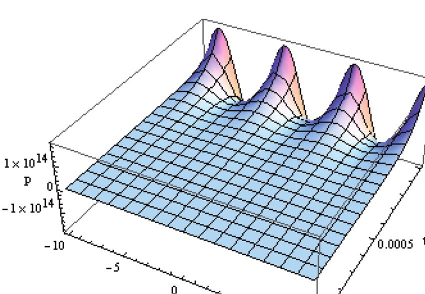
Morad et al.                                 A New Derivation of Exact Solutions for Incompressible Magnetohydrodynamic Plasma Turbulence

in collisional plasma has been the focus of many exper-              equations. Nonlinear dynamical processes assist us in com-
iments over the last few decades. In particular, when                prehending the nature and the structure formation of the
modeling plasma turbulence, the NS equations coupled                 turbulent. By using the complex ansatz method, the solv-
with Maxwell equations are important. However, MHD is                ability condition can be obtained as the model equation,
known to be the appropriate technique in the collisionless           the system can be solved to get the four cases.
case.4–6                                                                The goal of this research is to study the properties
   The aerodynamic and thermal dynamics of a New-                    of   nonlinear turbulent dynamics in incompressible one-
tonian incompressible fluid which has a constant prop-               dimensional       hydrodynamic and MHD turbulence by using
erty turbulent flowing through a high-performance two-               an  approximation       method that gives the ability to save the
dimensional channel of a horizontal heat transfer with               nonlinear     behaviors    of equations and provide the solutions
a rectangular cross-section were studied using computa-              of  small     amplitude     to describe long-range effects in the
                                 7 8
tional fluid dynamics (CFD). A numerical investigation               system.      Through     that,  a framework has been evaluated,
of a fluid’s dynamic and thermal dynamics with a con-                and    results   represented     in the figures, which have shown
stant property turbulent flowing through a two-dimensional           very    good    agreement      of  the governing parameters in the
horizontal rectangular channel was carried out by Menni              problem      within   the  researched    field.
et al. 9 10
              In this study, the upper surface was kept at a            This     work    introduces      an  accurate    analytical solution
constant temperature, while the lower surface was kept               for   analyzing     nonlinear     turbulent   systems   by driving the
warm.   11 12
               The internal structure of the channel’s thermal       MNLS        equation    for   the   model.    The   novel  model solu-
and dynamic analyses has been meticulously examined. In              tions    are  represented      by   assuming    that  the medium    can
                                                                     be treated as an MHD multi-fluid system. In the case of
Refs. [13–18], the authors encompassed diverse domains
                                                                     the MHD equations, to generate a single evolution equa-
of speed and heat, as well as distinct profiles of friction
                                                                     tion, the special assumptions and holding low order terms
and heat exchange coefficients in a channel with chang-
                                                                     must be chosen. The novelty of this study, that for the

                                                                                                                                               ARTICLE
ing walls. Abo-Dahab and Abdelhafez19 investigated the
                                                                     first time we explored the effect of the intrinsic magnetic
effects of magnetic field and thermal radiation on molyb-
                                                                     field on velocity and pressure fluctuations lately. And we
denum disulfide nanofluid combined. Mebarek and others
                                                                     extended that by applying RPM to achieve the examina-
studied an inclined ring filled with molten potassium, the
                                      IP: 192.168.39.151 On: Wed,    tion13ofOctsystem
                                                                                    2021parameters
                                                                                            10:20:36 associated with nonlinear terms
stability of natural convection, under the   influence of
                                           Copyright:       radial Scientific
                                                        American     in  the      Publishers
                                                                               differential    equations of NS turbulence and MHD
magnetism.19–21 The natural convection of MHD flow            of a byturbulence.
                                                       Delivered       Ingenta This technique determining the velocity fluc-
Newtonian nanofluid in a baffled enclosure of U-shaped is            tuation and studying the fluid pressure behavior.
investigated using a homogeneous single-phase nanofluid
model.22 23
   Transport phenomena in viscous and incompressible                 2. INCOMPRESSIBLE NAVIER-STOKES
fluid regimes adjacent to a spinning vertical cone of ther-               EQUATION
mal radiation and transpiration effects are studied using            For the simplest case, the equations reflect the bulk fluid
a mathematical model.24–26 Chamkha et al. studied the                velocity evolution v and the magnetic field B in an
incompressible steady flow properties such as viscosity,             incompressible flow with constant mass density may be
thermal radiation, conductivity, and viscous dissipation in          expressed as:2
order to treat a wide range of scientific and technologi-                      v                                1
cal problems.27–31 They also investigated the mass transfer                        + v · v = −  p +             B · B +  2 v (1)
                                                                               t                              4
of an electrically conducting fluid and simultaneous heat                     B
by combining stagnation convection flow on a flat plate                           + v · B = B · v +  2 B                         (2)
                                                                              t
embedded in the presence of magnetic field effects, fluid
                                                                     these equations are restricted because of the incompress-
wall blowing, and heat generation or absorption effects
                                                                     ibility condition and the magnetic field has solenoidal
which temperature-dependent, and in the presence of a
                                                                     character,
magnetic field, the flow of unsteady mixed convection over
                                                                                                 ·v = ·B = 0                           (3)
a vertical cone moving in a fluid layer with an angu-
lar velocity time-dependent was investigated. Dogonchi               Considering       the  limits   in   Eq. (3).  for  velocity and  mag-
et al.32 33 were the first to use a hybrid approach to inves-       netic field, p can measure easily. Therefore, beyond the
tigate the influence of a magnetic field on natural con-             incompressible limit, p is a passive quantity. Working with
vection in a cavity with an inclined elliptical heater with          a non-dimensional form of the MHD Eqs. set (1), (2) and
a nanoparticle form factor Significant factors’ impact on            (3) is beneficial. If the mean magnetic field assumed t be
flow and heat transfer characteristics are studied.   34 35         zero, all variables depend on two spatial parameter x and
   The “Reductive Perturbation Method” (RPM)        36 37
                                                           that is   time    t, and Eq. (1)–(3) take the following form:

a beneficial approach, that preserving the effects of non-              v                           1                           2
                                                                             + v·           v = − p+                 B·      B +  2 v (4)
linear, dispersive, and dissipative in relevant differential             t           x             x       4        x         x
J. Nanofluids, 10, 98–105, 2021                                                                                                         99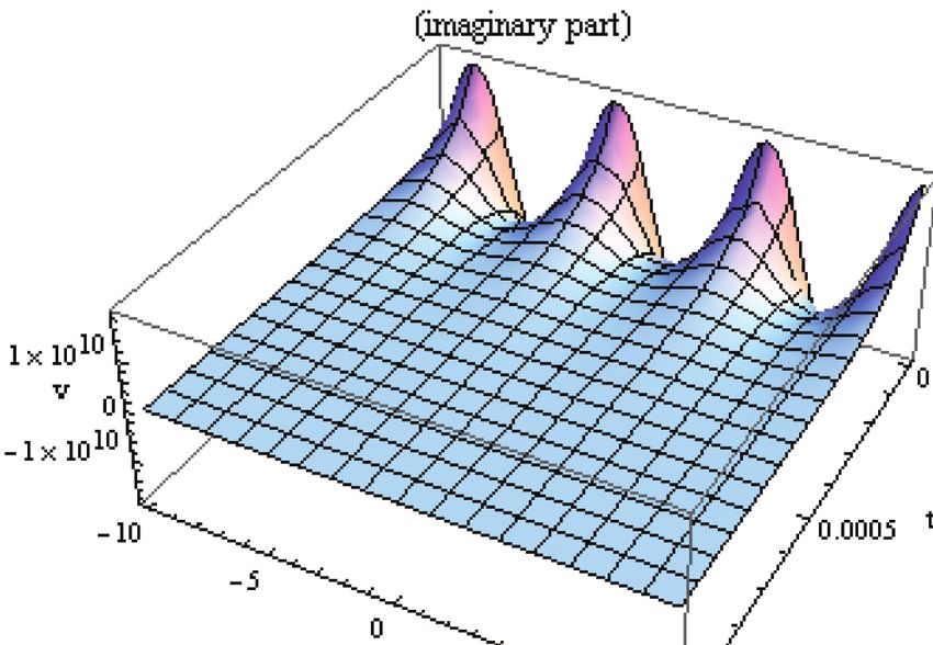
A New Derivation of Exact Solutions for Incompressible Magnetohydrodynamic Plasma Turbulence                                           Morad et al.


           B                       2
                                         2
                                                                                 x t, respectively. It is necessary to apply the following
              + v·     B = B·     v+      B                               (5)   partial relations,37
           t      x         x      x
                                                                                                  t = t − vgr  +            2
                                                                                                                                                       (12)
                ·v =    ·B = 0                                             (6)
             x      x                                                                             x = x +                                          (13)
          In this work, we assumed that the magnetic field acting in                              xx = xx + 2 x +              2
                                                                                                                                                       (14)

          the x direction takes a constant value Bx = constant, so the
          derivative of the magnetic field in this direction is always
                                                                                 3.1. First Order Approximation
          equal to zero, B/x = 0.
                                                                                 Using the RPM method by substituting Eq. (9)–(10) and
                                                                                 (11) into Eqs. (4)–(5) and (6), using the properties (12)–
          3. THE REDUCTIVE                                                       (13) and (14), a set of equations for all values of n and l
             PERTURBATION METHOD                                                 can be obtained. The different powers terms are collected:
          The reductive perturbation theory is presented as a solu-              For a harmonic at l = 1, the following results can be:
          tion method used to reduce a system of general nonlinear                          ik2  + v11
          hyperbolic to a solvable nonlinear single equation which            p11    =                        B11    = 0 (15)
                                                                                                     k
          defines a wide system.36 37 The approach of RPM used
          with more general systems, like dispersion or dissipation,          The importance of a harmonic at l = 1, comes in having
          demonstrates that they can be reduced to the Korteweg-           a basic relation, which is the dispersion relation, which
          de Vries equation (KdV) or the Burgers equation for long         links the wave number with the wave frequency,
          waves. It is also seen that the Schrödinger equation gov-                                    = −ik2                      (16)
          erns a wide field for the slow modulation propagation of an
ARTICLE

          infinitesimal amplitude plane wave and that a general wave       where  and  are unity. Eq. (16) shows that          can be
          system reduced to a nonlinear Schrödinger form equation          positive and this happens with the growth of time to cause
          for small and finite amplitudes, which are known as the          instability of the system while the        can take negative
          generalized nonlinear Schrödinger equation.                      values so that the system becomes stable with the decay
                                             IP: 192.168.39.151 On: Wed,   of 13  Oct 2021 10:20:36
             Now, the F is a state vector that       is implied
                                                   Copyright:
                                                                               time.
                                                                  to be Scientific
                                                               American               Publishers
          ui Bi pi  in space x and time t. The small deviations             The dispersion relation for the waveguide is a plot relat-
                                                              Delivered by Ingenta
          from the condition of equilibrium that are known as F 0 =        ing the characteristic wave vector of each k to the fre-
                   T
          0 1 1 . The state vector F expanded in a power series          quency of that wave. The phase velocity vph =  /k,
          of small parameter and has an expansion as,                      which   used to measure how fast a constant phase point is
                                                                           moving, and the group velocity vgr = −2ik measures how

                                               n n                         fast the wave energy is moving generally. In other words,
                               F =F0+           F                    (7)
                                          n=1
                                                                           the dispersion relation introduces stability properties of the
                                                                           MHD waves from the relation between vph and vgr , which
             And, F  F etc.: are functions of slow variables that
                     0   1                                                 provide   three cases of dispersion character. Moreover, the
          can be defined as:                                               dispersion   relation can be normal at vph /vgr > 1, while it
                                                                           is anomalous at vph /vgr < 1 and finally it is non-dispersive
                             = x − vgr t       = 2t               (8)   at vph = vgr . The dispersion relation shows us a basic per-
                                                                           ception of the system’s behavior if it is stable or not.
          vgr is the group velocity, that used to determine the veloc-        As shown in Figure 1, the dispersion relation represents
          ity along the modulation direction of the wave. The depen-       normal dispersion at vph > vgr , which gives good agree-

          dent variable can be expanded as F n =          n ilkx− t
                                                       l=− Fl e         , ment with the dispersion properties of the famous KdV
          then the problem physical quantities take the form,              equation in nonlinear hydrodynamic dispersive media.


                                 n


                                             n                                 3.2. Second Order Approximation
                      v=                    vl   eilkx−    t
                                                                           (9)
                           n=1       l=−                                        At this point we need four-wave components, for O 2 ,
                                                                                 the long-wave component of the orders l = 0 1 2 3 are


                                       n


                                                    n
                     p = 1+                        pl   eilkx−   t
                                                                          (10)   obtained, in the form:
                                 n=1       l=−                                                          10
                                                                                                   iv11


                                       n


                                                    n                                v12    =
                     B = 1+                        Bl   eilkx−   t
                                                                          (11)                          k
                                 n=1       l=−                                        B12    = 0
                                                                                                                 10  10
          The physical variables are considered real and be func-                                    ivgr v11    2i v11
          tions of the slow and fast independent variables    and                   p12    = −               +
                                                                                                             k            k2
          100                                                                                                            J. Nanofluids, 10, 98–105, 2021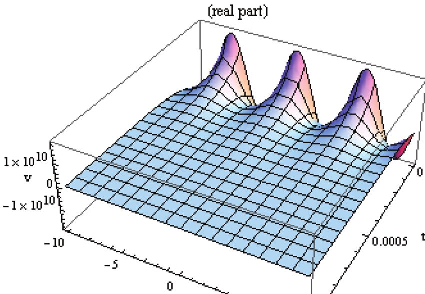
Morad et al.                                                                    A New Derivation of Exact Solutions for Incompressible Magnetohydrodynamic Plasma Turbulence

                                                        Dispersion relation                                 partial differential equations that are being studied and
                          0                                                        ← (KdV) vph
                                                                  KdV vgr →                                 constructed. The articles present a range of interesting
                                                                                                            techniques, including inverse scattering theory, sin-cosine
                                                                                                            method, expanded tanh-function method, and other.38–40
The wave frequency, Ω

                         –5

                                                            ← (MHD) vph
                                                                                                            4. THE EXACT SOLUTIONS OF NLS
                        – 10              (MHD) vgr →
                                                                                                               EQUATION
                                                                                                            In this section, the complex ansatz method is proposed to
                                                                                                            obtain the exact complex traveling wave solutions of NLS
                                                                                                            without converting them into real and imaginary parts. The
                        – 15
                                                                                                            partial differential equation is given by Refs. [37, 38];
                                0             1                   2                 3                 4

                                                                                                                              f v vx  vt  vxx     = 0
                                                          The wavenumber, k
                                                                                                                                                                       (20)
Fig. 1. The relation between v and k of our MHD model in comparison
with the KdV dispersion properties.                                                                         By using the complex transformation,

                               v22    = 0                                                                                           = iK −                      (21)
                                        kv11   2                                                         Equation (21) can convert the partial differential Eq. (20)
                               b22    =
                                       −ik2  − 2                                                           into ordinary differential equation (ODE)
                                        kv11   2
                           p22    =                                                                                  gv iKv  −iv − K 2 v     = 0      (22)
                                       −ik2  − 2

                                                                                                                                                                               ARTICLE
                           v32    = 0 b32    = 0                        p32    = 0          (17)
                                                                                                            The suggested solutions could be;
   The second-order of O  and l = 1; that is an impor-      2

tant step in the solution by the method of reduction per-            v = li=0 ai F i  + li=1 bi F i−1 Gi  (23)
                                  IP: 192.168.39.151 On: Wed, 13 Oct 2021 10:20:36
turbation, as it results in the compatibility condition,
                                        Copyright:        and Scientific Publishers
                                                    American   By making the balance of the highest order linear term,
this is an important role in calculating the group Delivered
                                                   velocity. by Ingenta
                                                               the constants ai  bi , and the integer l can be determined.
                                                              The coupled Riccati equations will be,
                     vgr = −2ik =                       (18)
                                     k
                                                                                   F  = −F G                  (24)
vgr is a characteristic of a dispersive medium, it used to
determine how the medium will affect a wave traveling          And,
through it.                                                                           G  = 1 − G2                (25)

3.3. Third Order Approximation                                                                              The two types of solution are admitted as:
By using derived equations in the order O 3 with
first harmonic mode l = 1, the solvability condition was                                                              F  = ±sech            G = tanh      (26)
obtained by the model equation,
                                                                                                            The relation between F  and G is G2 = 1 − F 2 , and,
 i v11    + P   v11    + Qv11   2 v11    = 0
                                                          (19)                                                        F  = ±csch            G = coth      (27)
which is the well-known envelope MNLS equation with
                                                                                                               The exact solutions for Eq. (20) can be produced by
real coefficients P and Q; it describes the evolution of
                                                                                                            substituting Eq. (23) into Eq. (22), using Eq. (25) repeat-
the envelope of the modulated wave group. The dispersion
                                                                                                            edly with Eqs. (26) or (27) and by setting each coefficient
coefficients P and Q are satisfied by;
                                                                                                            of F i and GF i to zero which results in a set of linear equa-
                                    2kvgr − 3                                 2 k3                        tions for each  K ai  bi , these equations are solved to
                         P=                              Q=
                                         k2                         −k4 2 + ik2        +2      2          give us the ODE form of Eq. (20).

   Equation (19) can be considered as the modified non-                                                                    −iv + P K 2 v + Qv2 v = 0                (28)
linear Schrördinger equation (MNLS), because of its sym-

metry of NLS in quantum mechanics theory which is                                                           The balancing between v and v2 v yields l = 1, as this
nonlinear equation and has great interest. This equation                                                    indicates the following form of the solution
can be used in plasma waves and nonlinear optics. Here,
exact solutions are carried to both linear and nonlinear                                                                         v = a0 + a1 F + b1 G                  (29)

J. Nanofluids, 10, 98–105, 2021                                                                                                                                       101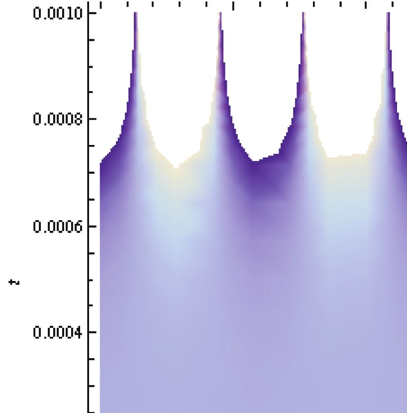
A New Derivation of Exact Solutions for Incompressible Magnetohydrodynamic Plasma Turbulence                                             Morad et al.

             Use Eq. (26) with F ∗ = F and G∗ = −G, substitute                         number and is the ratio of the velocity of system particles
          Eq. (29) into Eq. (28) and evaluate the coefficients of both                 to the speed of sound in the fluid.41
          F i and GF i to zero, we obtain
                                                                                                                           v2 1/2
                Qa30 − Qa0 b12 = 0       −a1 + 2Qa0 a1 b1 = 0                                                   Ms =                                   (30)
                                                                                                                             Cs
                3Qa0 a21 + b1 + Qa0 b12 = 0
                                                                        In incompressible flow,42 we can say that plasma moving at
               −K   2
                        P a1 + 3Qa20 a1 − Qa1 b12
                                             = 0                       low Mach numbers, so the material derivative is qual zero
               2K P a1 + Qa1 + Qa1 b1 = 0 Qa0 b1 − Qb1 = 0
                  2           3        2            2       3           and the plasma density remains constant with the applica-
                                                                        tion of pressure on the system. When it takes values less
               a2K 2 P b1 + Qa21 b1 + Qb13 = 0                          than 1, the bulk particle’s velocity is small in compari-
             The following given cases are produced by solving these    son to the speed of sound. In fluid dynamics, when the
          algebraic equations;                                          divergence of the flow velocity is zero  . v = 0, a flow is
                                     √ √                                considered   incompressible. Solutions involving small per-
                                    i 2K P                              turbation  in density and pressure fields are agreed by the
                case 1      a0 = − √              a1 = 0
                                         Q                              differing density set and may allow pressure stratification
                                     √ √                                in the domain.
                                    i 2K P
                            b1 = − √              = 2K 2 P                As seen in Figure 2, the system appears homogeneous
                                         Q                              horizontally, so that it becomes clear that the velocity is
                                   √ √
                                  i 2K P                                constant in both x and t, so that the velocity is induced to
                case 2      a0 =     √         a1 = 0                   a sudden rise until it reaches a maximum value by increas-
                                       Q
                                     √ √                                ing time and this disturbance is noticeable around the axis
                                    i 2K P                              of space x. This increase in the velocity occurs due to
                            b1 = − √              = −2K P
ARTICLE

                                                           2
                                         Q                              the formation of vortex waves. The velocity in hydrody-
                                     √ √                                namic turbulence consists of both compression and vortex
                                    i 2K P
                case 3      a0 = − √              a1 = 0                motions.
                                         Q IP: 192.168.39.151 On: Wed, 13 Oct 2021 10:20:36       v = v⊥ + v
                                   √ √
                                  i 2K P         Copyright:   American Scientific Publishers
                            b1 =     √          = −2K 2 P Delivered bywhere
                                                                         Ingentav which is longitudinal, curl-free, and leads to
                                       Q                                shocks, v⊥ is rotational, divergence-free, and is associ-
                                   √ √
                                  i 2K P                                ated with vortex structures. A solenoidal flow velocity field
                case 4      a0 =     √         a1 = 0                   defines an incompressible flow. But besides having zero
                                       Q
                                   √ √                                  divergence, a solenoidal field also has the extra connota-
                                  i 2K P                                tions of having a non-zero curl (i.e., rotational component),
                            b1 =     √          = 2K P 2
                                       Q                                meaning that the flow is mainly solenoidal at the subsonic
                                                                        and incompressible limit.
                                                                           Figures 2 and 3 show that the flow quantities v are
          5. MACH NUMBER AND ITS                                        homogeneous, where the upstream and downstream of
              CONSEQUENCES                                              these vortex waves should be considered stationary in sys-
          The magnitude of many of the compressibility effects is       tem reference transition layers. The flow is initialized with
          determined by Mach number which is the dimensionless          a constant mass-density and zero flow velocity. For large

          Fig. 2. Space-time plot of the velocity real and imaginary parts in the case of our mode at K = 01 m, k = 01 m,  = 10−4 m2 /s, and  = 102 m2 /s.

          102                                                                                                               J. Nanofluids, 10, 98–105, 2021
Morad et al.                                      A New Derivation of Exact Solutions for Incompressible Magnetohydrodynamic Plasma Turbulence

                                                                               distinctive feature of incompressible flow. By looking at
                                                                               the behavior of the velocity inside the system, it becomes
                                                                               clear to us that the magnetic field applied to the system
                                                                               is constant, and this led to the homogeneity of the veloc-
                                                                               ity field until an intrinsic magnetic field occurred within
                                                                               the system which lead to sudden fluctuations of the veloc-
                                                                               ity waves. This intrinsic magnetic field is responsible for
                                                                               many changes that occur within the system, including the
                                                                               behavior of pressure as well.

                                                                               6. PRESSURE DETERMINATIONS
                                                                        In nature, there is no incompressible fluid. In nanofluids,
                                                                        this is frequently the case. When the pressure variation
                                                                        is small compared to the absolute pressure, we can con-
                                                                        sider gases incompressible. It is easy to obtain solutions
                                                                        for pressure values, which of course are identical to the
                                                                        boundary solutions for velocity in the same declared sys-
Fig. 3. The graph shows the velocity solution release due to the vortex tem. The total pressure may satisfy either the normal com-
waves in plasma in incompressible case.
                                                                        ponent at the walls, or the tangential component of it, but
                                                                        not both. The thing that is worth pointing out, the incom-
scale, the solenoid force infuses energy and course the                 pressible fluid means that it has a constant density and
turbulent flow after dynamic times and statistically sta-               has a low Mach. The first means that the density does not

                                                                                                                                                         ARTICLE
tionary. The transition to turbulence is taken into account             change at all, but the second means that the field veloc-
and reveals significance in time. This hydrodynamic tur-                ity is small compared to the speed of sound, but it allows
bulence behavior can be explained by the sudden change                  the density to change as a function of temperature and not
in the dissipation of kinetic energy    IP: induced   by the vortex
                                            192.168.39.151              pressure.
                                                                  On: Wed,  13 Oct 2021 10:20:36
waves.                                        Copyright: American Scientific
                                                                           After aPublishers
                                                                                    period of time stage in which the fluid is able to
   The intrinsic magnetic field generated by Delivered        moving byslide
                                                                          Ingenta
                                                                               at the wall, the velocity field presented in Figure 2
nanoparticles is responsible for producing steepen vortex               does not contribute to one that the Navier boundary con-
waves. These vortex waves are fluctuated and have a finite              dition obeys. The relation between the rate of shear at the
amplitude and can steepen into being a jump and be a                    wall and the slip velocity can be measured if the veloc-
layer. This layer is a thin transition and these waves move             ity field is advanced in time with the pressure, after the
faster than the related to the linear group velocity of the             initial time step, change with x sinusoidally. The behav-
underlying waves and showed a local plane. One can con-                 ior of the pressure, as shown in Figure 4, is very similar
sider upstream and downstream of these vortex planes for                to the behavior of the velocity field, and this is due to
the flow quantities v to be homogeneous and can also be                 the pressure being greatly affected by the velocity of the
stationary in transition layers of system reference.                    system particles, where the pressure appears homogeneous
   In the other words, the speed with which the particles               in both time t and direction x until it has clear distur-
move is the Alfvén velocity, and this velocity is a basic and           bances at a certain time that the intrinsic magnetic field

Fig. 4.   Space-time plot of the pressure real and imaginary parts in the case of our mode at K = 01 m, k = 01 m,  = 10−4 m2 /s, and  = 102 m2 /s.

J. Nanofluids, 10, 98–105, 2021                                                                                                                   103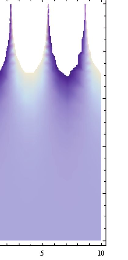
A New Derivation of Exact Solutions for Incompressible Magnetohydrodynamic Plasma Turbulence                              Morad et al.

                                                                                  which the solutions of that model represent rising in the
                                                                                  velocity due to the occurrence of the vortex wave. Initially,
                                                                                  the system remains horizontally homogeneous and occurs
                                                                                  physically sudden rising in the velocity occurs and growth
                                                                                  until it reaches its maximum value with increase in the
                                                                                  time at t > 0  001s and perturbed about the space axis.
                                                                                  There is good agreement of the velocity behavior between
                                                                                  our results and the previous measurements under the effect
                                                                                  of a constant magnetic field. Therefore, one can say that
                                                                                  the velocity field has an identity of great importance and
                                                                                  a clear influence on the characteristics of the studied
                                                                                  system.42
                                                                                  (iii) The disturbances in both velocity and pressure of
                                                                                  the system appeared at t > 0  001 s and 0.5 m < x <
                                                                                  0.5 m, which occur as a result of configuring the intrinsic
                                                                                  magnetic field is generated by moving particles. More-
          Fig. 5. The graph shows the 2D pressure plasma solution in both time
                                                                                  over, this intrinsic magnetic field controls various sys-
          t and space x for incompressible case.
                                                                                  tem properties for spreading i.e., viscosity, pressure, and
                                                                                  nonlinearity.
          controls these disturbances. Figures 4 and 5 clarify that               (iv) In the turbulent incompressible system, their 2D
ARTICLE

          the pressure profile is a process that has the characteristics          plane-like spatial cover all scales of spatial length. There-
          of random homogeneity. It can be assumed that the term                  fore, vortex coupled with velocity fluctuation on all spatial
          for describing pressure fluctuations when using the MNLS                scales. Moreover, the small-amplitude waves propagate in
          equation is small if compared to       IP:the other terms ofOn:
                                                     192.168.39.151               the13cold
                                                                           the Wed,      Oct plasma  are governed by the KdV equation and
                                                                                              2021 10:20:36
          MNLS equation. Using this assumption,        Copyright:
                                                          one can American
                                                                    consider Scientific
                                                                                  waves are  Publishers
                                                                                               vortex waves of the MNLS equation that can
          the quasi-adiabatic evolution of these vortex waves      Delivered
                                                                          and bybehave
                                                                                   Ingentaas KdV solutions. Finally, the drawn figures have
          derive the equation to help us in this evolution description            shown very good agreement within the investigated area of
          which gives a good agreement with the results introduced                the governing parameters in the problem. We recommend
          in Ref. [43].
                                                                                  that there be a lot of studies to clarify the extent of the
             Figure 5 presents the vortex waves of the pressure
                                                                                  stability of this system and the factors affecting its stabil-
          propagation with homogeneous random processes and
          also shows that the distribution of pressure after a short              ity. It is also possible to study the effect of the magnetic
          period of the fluctuations which have steepened into the                Prandtl number and the relationship of this number to the
          vortex.                                                                 stability of the system. And there could be future works
                                                                                  that will focus on the other phenomena in nanofluids
                                                                                  flow.
          7. CONCLUSIONS AND FUTURE WORK
          In the present study, we studied the small-amplitude per-
          turbations behavior in cold plasma. MHD equations, along              Highlights
          with the state equation was developed by using the RPM.               • The governing equations that describe plasma turbu-
          Therefore, we can say that the medium can be thought of               lence term were solved exactly.
          as a system of multifluid MHD. As a consequence, a non-               • The solution can be applied to understand several flow
          linear wave equation with a modified form of the deriva-              systems.
          tive nonlinear Schrödinger equation is obtained. The key              • The average velocity of the turbulent fluctuations is
          remarks of the present work are as follows:                           smaller than the velocity of sound in the medium, which
          (i) Analytical studies of isotropic incompressible tur-
                                                                                leads to disturbances in velocity waves.
          bulence in the non-magnetic case are presented to
                                                                                • The intrinsic magnetic field was generated by moving
          describe the properties of hydrodynamic turbulence such
          as the velocity, pressure, and Mach number of the                     particles while lead to the disturbances.
          flow.                                                                 • The fluctuations produce changes in the properties of
          (ii) In incompressible hydrodynamic turbulence, the rel-              the turbulence to a large extent.
          ative importance of vortex-related motions over shock                 • These properties were studied and presented in the
          motions is likely to depend on the velocity field are present         manuscript.

          104                                                                                                  J. Nanofluids, 10, 98–105, 2021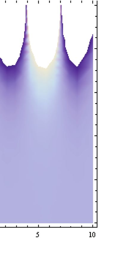
Morad et al.                                   A New Derivation of Exact Solutions for Incompressible Magnetohydrodynamic Plasma Turbulence

NOMENCLATURE                                                             11. Y. Menni, A. Azzi, and A. J. Chamkha, J. Brazil. Soc. Mech. Sci.
      v Velocity component along x axe                    m/s              Eng. 12, 3888 (2018).
                                                                         12. Y. Menni, A. Chamkha, C. Zidani, and B. Benyoucef, Math. Model.
      t Time                                              (s)
                                                                             Eng. Probl. 6, 52 (2019).
     B Applied magnetic field                             (Wb/m2 )       13. Y. Menni, A. J. Chamkha, A. Azzi, and C. Zidani, International
     p Fluid pressure                                     P a              Journal of Fluid Mechanics Research 47, 23 (2020).
    Re Reynolds number                                    –              14. Y. Menni, A. Azzi, and A. J. Chamkha, Heat Transfer Research 50,
    Bx Magnetic field acting in the x direction           (Wb/m2 )           1781 (2019).
                                                                         15. Y. Menni, A. J. Chamkha, A. Azzi, and B. Benyoucef, World J.
      k Wavenumber                                        m                Model Simul. 15, 213 (2019).
     L Length scale                                       m            16. Y. Menni, A. Chamkha, G. Lorenzini, and B. Benyoucef, Mathemat-
    Ms Mach number                                        –                  ical Modelling of Engineering Problems 6, 170 (2019).
    Cs Speed of sound in the fluid                        (m/s)          17. Y. Menni, A. J. Chamkha, and A. Azzi, J. Comput. Appl. Mech. 6,
    vgr Group velocity                                    (m/s)              741 (2020).
                                                                         18. J. Raza, F. Mebarek-Oudina, and A. J. Chamkha, Multidiscipline
     P Dispersion coefficient in NLS                      −                  Modeling in Materials and Structures 15, 737 (2019).
     Q Nonlinearity coefficient in NLS                    −              19. M. Abo-Dahab, M. A. Abdelhafez, F. Mebarek-Oudina, and S. M.
ai , bi Constants are defined in Eq. (23)                 –                  Bilal, Indian Journal of Physics 95, 1 (2021).
     K Wavenumber of the new model equation               (m)            20. F. Mebarek-Oudina, R. Bessaih, B. Mahanthesh, A. J. Chamkha, and
                                                                             J. Raza, Int. J. Numer. Methods Heat Fluid Flow 31, 1172 (2020).
                                                                         21. A. K. Abu-Nab, E. S. Selima, and A. M. Morad, Physica Scripta
Greek Symbols                                                                96, 035222 (2021).
  Magnetic resistivity                                       (m2 /s)    22. A. Zaim, A. Aissa, F. Mebarek-Oudina, B. Mahanthesh, G.
                                                                             Lorenzini, M. Sahnoun, and M. El Ganaoui, Propulsion and Power
  Kinematic viscosity                                        (m2 /s)
                                                                             Research 9, 383 (2020).
    Wave frequency                                            (1/s)      23. R. Slimani, A. Aissa, F. Mebarek-Oudina, U. Khan, M. Sahnoun,
 Angular frequency of the new model equation (rad/s)                        A. J. Chamkha, and M. A. Medebber, Eur. Phys. J. Appl. Phys. 92,

                                                                                                                                                  ARTICLE
                                                                             10904 (2020).
                                                                         24. M. A. Ismael, T. Armaghani, and A. J. Chamkha, J. Taiwan Inst.
ABBREVIATIONS                                                                Chem. Eng. 59, 138 (2016).
RPM—Reductive perturbation method; NS—Navier-                            25. M. Veera Krishna, and A. J. Chamkha, Results in Physics 15, 102652
                                        IP: 192.168.39.151
Stokes equations; MHD—Magnetohydrodynamic;                   KdV—On: Wed, 13    Oct 2021 10:20:36
                                                                             (2019).
                                              Copyright: American Scientific
The Korteweg-de Vries equation; HD—Hydrodynamic;                                     Publishers
                                                                         26. Y. Menni,  A. J. Chamkha, and A. Azzi, Special Topics and Reviews

ODE—Ordinary differential equation; PDF—Partial dif-       Delivered   by Ingenta
                                                                             in Porous Media—An International Journal 10, 49 (2019).
                                                                         27. M. Ghalambaz, A. Doostani, E. Izadpanahi, and A. J. Chamkha, J.
ferential equation; NLS—Nonlinear Schrördinger equa-                         Therm. Anal. Calorim. 139, 2321 (2020).
tion; MNLS—Modified nonlinear Schrördinger equation.                     28. B. Kumar, G. S. Seth, R. Nandkeolyar, and A. J. Chamkha, Int. J.
                                                                             Therm. Sci. 146, 106101 (2019).
Conflicts of Interest                                                    29. A. J. Chamkha, M. A. Mansour, A. M. Rashad, H. Kargarsharifabad,
                                                                             and T. Armaghani, J. Thermophys. Heat Transfer. 34, 836 (2020).
There are no conflicts to declare.
                                                                         30. A. J. Chamkha and A. A. Khaled, Int. J. Numer. Methods Heat Fluid
                                                                             Flow 10, 94 (2000).
Acknowledgments: The authors would like to thank                         31. H. S. Takhar, A. J. Chamkha, and G. Nath, Heat Mass Transfer 39,
the editor and anonymous referees.                                           297 (2003).
                                                                         32. A. S. Dogonchi, T. Armaghani, A. J. Chamkha, and D. D. Ganji,
                                                                             Arab. J. Sci. Eng. 44, 7919 (2019).
References and Notes                                                     33. A. S. Dogonchi and D. D. Ganji, Journal of the Taiwan Institute of
 1. M. Lesieur, Turbulence in Fluids. Kluwer Academic Publishers, Dor-       Chemical Engineers 69, 1 (2016).
    drecht (1997).                                                       34. Y. Menni, A. J. Chamkha, and A. Azzi, J. Nanofluids 8, 893
 2. D. Biskamp, Magnetohydrodynamical Turbulence. Cambridge Uni-             (2018).
    versity Press, Cambridge, (2003).                                    35. Y. Menni, A. Chamkha, G. Lorenzini, N. Kaid, H. Ameur, and M.
 3. G. Belmont, L. Rezeau, C. Riconda, and A. Zaslavsky, Introduction        Bensafi, Mathematical Modelling of Engineering Problems 6, 415
    to Plasma Physics. Elsevier, ISTE Press, United Kingdom (2019).          (2019).
 4. T. Z. Abdel Wahid and A. M. Morad, Applied Advances in Mathe-        36. A. M. Morad, M. Abu-Shady, and G. I. Elsawy, Physica Scripta 95,
    matical Physics, 2020, 1289316 (2020).                                   025205 (2020).
 5. E. M. Elsaid, T. Z. Abdel Wahid, and A. M. Morad, Results in         37. E. S. Selima, Y. Mao, Y. Xiaohua, A. M. Morad, T. Abdelhamid,
    Physics 19, 103554 (2020).                                               and B. I. Selim, Appl. Math. Model 57, 376 (2018).
 6. T. Z. Abdel Wahid and A. M. Morad, IEEE Access 8, 76423 (2020).      38. A. M. Abourabia and A. M. Morad, Physica A. 437, 333 (2015).
 7. Y. Menni, A. Chamkha, C. Zidani, and B. Benyoucef, Int. J. Numer.    39. A. M. Abourabia, T. S. El-Danaf, and A. M. Morad, Chaos, Solitons
    Methods Heat Fluid Flow 30, 3027 (2019).                                 and Fractals 41, 716 (2009).
 8. Y. Menni, A. Chamkha, G. Lorenzini, N. Kaid, H. Ameur, and M.        40. A. M. Morad, E. S. Selima, and A. K. Abu-Nab, European Physical
    Bensafi, Mathematical Modelling of Engineering Problems 6, 15            Journal Plus 136, 306 (2021).
    (2019).                                                              41. G. Gogoberidze, Phys. Plasmas 14, 022304 (2007).
 9. Y. Menni, A. Azzi, A. J. Chamkha, and S. Harmand, Int. J. Numer.     42. F. H. Shu, Physics of Astrophysics, University Science Books, Vol-
    Methods Heat Fluid Flow 29, 3908 (2019).                                 ume II: Gas Dynamics (A Series of Books in Astronomy). Mill
10. Y. Menni, A. Azzi, A. J. Chamkha, and S. Harmand, J. Comput.             Vallye, CA. ISBN: 0935702652 (1992).
    Appl. Mech. 5, 231 (2019).                                           43. B. T. Kress and D. C. Montgomery, J. Plasma Phys. 64, 371 (2000).

J. Nanofluids, 10, 98–105, 2021                                                                                                          105
You can also read