Animating Hair with Loosely Connected Particles
←
→
Page content transcription
If your browser does not render page correctly, please read the page content below
EUROGRAPHICS 2003 / P. Brunet and D. Fellner                                                                                Volume 22 (2003), Number 3
(Guest Editors)

                 Animating Hair with Loosely Connected Particles

                                Yosuke Bando†                                  Bing-Yu Chen‡                  Tomoyuki Nishita

                                                                       The University of Tokyo
                                                            {ybando, robin, nis}@nis-lab.is.s.u-tokyo.ac.jp

         Abstract
         This paper presents a practical approach to the animation of hair at an interactive frame rate. In our approach,
         we model the hair as a set of particles that serve as sampling points for the volume of the hair, which covers the
         whole region where hair is present. The dynamics of the hair, including hair-hair interactions, is simulated using
         the interacting particles. The novelty of this approach is that, as opposed to the traditional way of modeling hair,
         we release the particles from tight structures that are usually used to represent hair strands or clusters. Therefore,
         by making the connections between the particles loose while maintaining their overall stiffness, the hair can be
         dynamically split and merged during lateral motion without losing its lengthwise coherence.
         Categories and Subject Descriptors (according to ACM CCS): I.3.7 [Computer Graphics]: Three-Dimensional
         Graphics and Realism, I.3.3 [Computer Graphics]: Picture/Image Generation

1. Introduction
The ability to represent realistic-looking hair plays a crucial
role in the synthesis of life-like human models. However,
the enormous number (a human scalp typically has 100,000
strands) and thin nature of hair strands complicate and slow
down all of the processes for hair image generation, includ-
ing modeling, rendering and animation. Moreover, when we
want to animate hair based on a physically plausible simu-
lation, the situation is even worse, because we have to take
into account interactions among the hair strands (so-called                                      (a)                  (b)                 (c)
hair-hair interactions) in order to reproduce realistic behav-
ior of the hair, as many researchers have already pointed                               Figure 1: (a) The hair that we wish to represent. (b) The
out4, 10, 13, 16, 20, 22 . The complex behavior of hair results from                    particles are distributed as sampling points for the volume
the characteristics of individual hair strands and the inter-                           of the hair. (c) Traditional methods often represent the hair
actions between them such as collisions, friction, repulsion                            as serial chains of connected particles (the same number of
due to static electricity and cohesion/adhesion due to lipids                           particles as (b)).
or hair-dressings21 . Hair-hair interactions are therefore es-
sential when animating hair. However, computing the inter-
actions among a large number of individual hair strands is                              a reasonable cost. Traditionally, hair is modeled using fixed
still expensive with the computer power currently available.                            structures that represent hair strands or clusters, such as se-
   In this paper, a practical method is proposed for animat-                            rial chains of connected points or particles. In contrast, we
ing hair while taking into account hair-hair interactions at                            use unordered particles that have only loose connections to
                                                                                        those nearby. Thus we call them loosely connected parti-
                                                                                        cles, or LCP. The particles serve as sampling points that
† In Toshiba Corporation since April 2003.                                              track the motion of the volume of the hair, and the dynamics
‡ In National Taiwan University since August 2003.                                      of the hair, including hair-hair interactions, is simulated us-

 c The Eurographics Association and Blackwell Publishers 2006. Published by Blackwell
Publishers, 108 Cowley Road, Oxford OX4 1JF, UK and 350 Main Street, Malden, MA
02148, USA.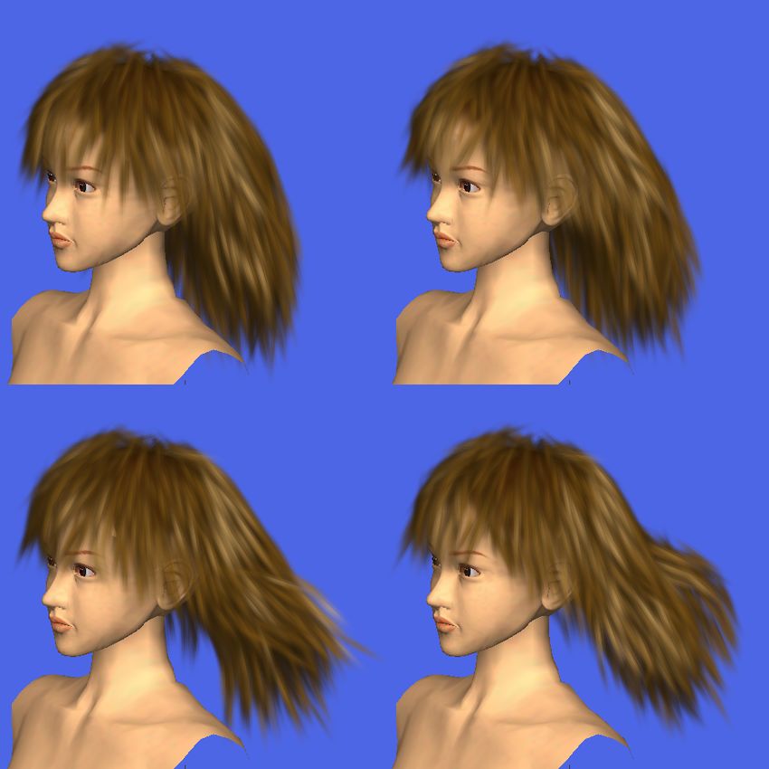
Bando, Chen, and Nishita / Animating Hair with Loosely Connected Particles

ing the interacting particles. Each particle represents a cer-            Hadap and Magnenat-Thalmann10 animated hair with
tain amount of the hair medium around it, and it might be              generalized hair-hair interactions. They assumed that hair
viewed as a volume density. This notion, inspired by Hadap             is a continuum and elegantly handled hair-hair interactions
and Magnenat-Thalmann10 , is illustrated in Figure 1.                  using particle-based fluid dynamics. However, the computa-
                                                                       tional cost was still high because they modeled individual
   Representing hair by using sampling points can be re-
                                                                       hair strands explicitly with serial chains of rigid segments
garded as an approximation or simplification of a collection
                                                                       (10,000 strands with 30 segments each) and glued several
of individual hair strands in order to reduce the high com-
                                                                       particles to each of the segments, so that the amount of com-
putational cost of checking and evaluating hair-hair interac-
                                                                       putation was huge (2 minutes per frame). The results were
tions. From this point of view, one might think of a more typ-
                                                                       excellent, but not to the extent that they captured the discon-
ical approach, i.e., to bring several strands together to form a
                                                                       tinuities of hair. Our LCP approach can be viewed as freeing
cluster or wisp and to then model each cluster as some struc-
                                                                       the particles from these serial chains.
tured element, such as a generalized cylinder. This is justifi-
able because the hair strands tend to clump together, which               Koh and Huang15 modeled hair clusters as strips of
is one of the frequently observed phenomena resulting from             spline surfaces and avoided collisions by introducing springs
hair-hair interactions, and clustering effects are therefore im-       among them. Plante et al.20 simulated interactions among
portant for producing natural-looking hair images. However,            the hair clusters, each of which was modeled as a skele-
as Kim and Neumann14 pointed out, clustering is not a static           ton and its envelope. The skeleton captures the lengthwise
phenomenon. When hair moves, the hair-hair interactions                shape of the cluster, whereas its envelope captures the cross-
cause clusters to split and merge dynamically. To simulate             sectional shape deformation. Chang et al.4 simulated only a
this, we could subdivide the structured elements to construct          small number of hair strands called guide hairs, and interpo-
a hierarchical tree structure of clusters, as in their multi-          lated the rest. They handled hair-hair interactions with auxil-
resolution hairstyle modeling (MHM) system. However, it is             iary triangle strips spanning the nearby strands. These three
unclear how we can split and merge the clusters at different           methods are similar in spirit. They reduce the number of hair
levels in different sub-trees. Although we can animate the             strands to be computed (in the form of strips, skeletons, and
highest resolution clusters individually, this severely limits         guide hairs, respectively) in order to speed up the simulation
the number of clusters available in order to handle hair-hair          and also to capture the discontinuities of hair. Moreover, the
interactions with a reasonable computation time.                       gaps among the sparse hair strands are compensated for by
   For this reason, we do not arrange the particles to form            additional structures such as springs, envelopes and auxiliary
a fixed set of clusters, but distribute them in an unordered           triangle strips, respectively. We also take a similar approach,
manner throughout the hair volume. The hair is rendered                but since the particles are distributed over the hair volume
by placing billboards with hair texture at the positions of            as shown in Figure 1 (b), the gaps between the particles are
the particles, oriented by a hair direction vector maintained          small. Besides, compensation for these gaps, which actually
with each particle. To simulate dynamic clustering effects,            models hair-hair interactions, is performed through particle
the neighboring particles should have coherence and move               dynamics rather than by introducing additional structures.
together to some extent. Moreover, the neighboring particles           The method by Koh and Huang15 achieved real-time ani-
should also be able to draw apart, since they do not represent         mation, but the springs accounting for hair-hair interactions
portions of the hair volume that are occupied by exactly the           were simplistic and imposed strong restrictions on free lat-
same set of hair strands. Therefore, some looseness in the             eral motion of the hair. The methods proposed by Plante et
connections between the particles is essential. Results show           al.20 and Chang et al.4 took up to tens of seconds to obtain
that our LCP approach can successfully reduce the compu-               the final rendered image.
tational cost of animating hair without losing most of the
characteristics resulting from hair-hair interactions.
                                                                       3. Modeling Hair with LCP
2. Related Work                                                        3.1. Overview
In this section, we limit our review to previous work on
                                                                       Hair is modeled as a set of particles that serve as sampling
the animation of hair that takes into account hair-hair in-
                                                                       points for the volume of the hair. Particle i has mass mi , po-
teractions. Interested readers may refer to the survey by
                                                                       sition xi and velocity vi , just like a standard particle system.
Magnenat-Thalmann et al.17 and Kim’s dissertation12 .
                                                                       The mass indicates the amount of hair medium that the par-
   Several works have modeled specific aspects of hair-hair            ticle represents and the distribution of the particle mass in
interactions. Kim and Neumann13 added some constraints to              space determines the density of the hair. The density here
hair strands by enclosing a hair surface within a thin bound-          indicates the amount of hair medium in a unit volume, as
ing volume. Lee and Ko16 gave hair body by prohibiting                 distinguished from the density of the hair material. As de-
hair strands from penetrating inside layers defined around             scribed by Hadap and Magnenat-Thalmann10 , we borrow an
the head.                                                              idea from smoothed particle hydrodynamics (SPH)18, 6 , and

                                                                                        c The Eurographics Association and Blackwell Publishers 2006.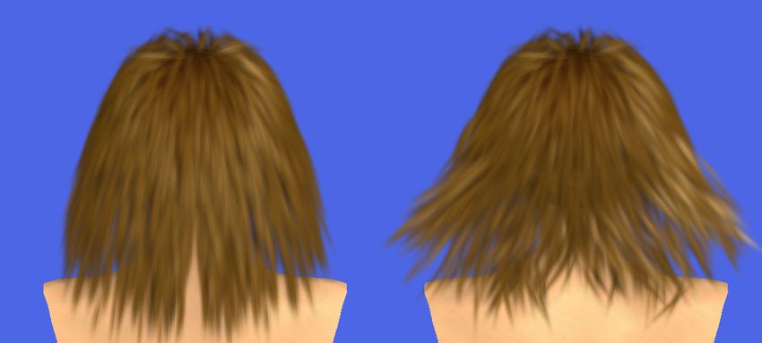
Bando, Chen, and Nishita / Animating Hair with Loosely Connected Particles

the density ρi at position xi is computed as follows:                          from the head model with four Catmull-Rom spline curves3
                                                                               by specifying their control points interactively. Then we em-
                     ρi = ∑ m jW (||x j − xi ||, h),                  (1)
                              j
                                                                               bed the scalp surface in a unit square domain D : [0, 1]×[0, 1]
                                                                               with axes u and v as shown in Figure 2 (b), using a piece-
where j runs through all of the particle indices and W repre-                  wise linear approximation of harmonic mapping8 . If we de-
sents an interpolating kernel called a smoothing kernel. We                    note this mapping from world space to the parameter do-
assume that the particles are smeared out in space so that                     main by φ :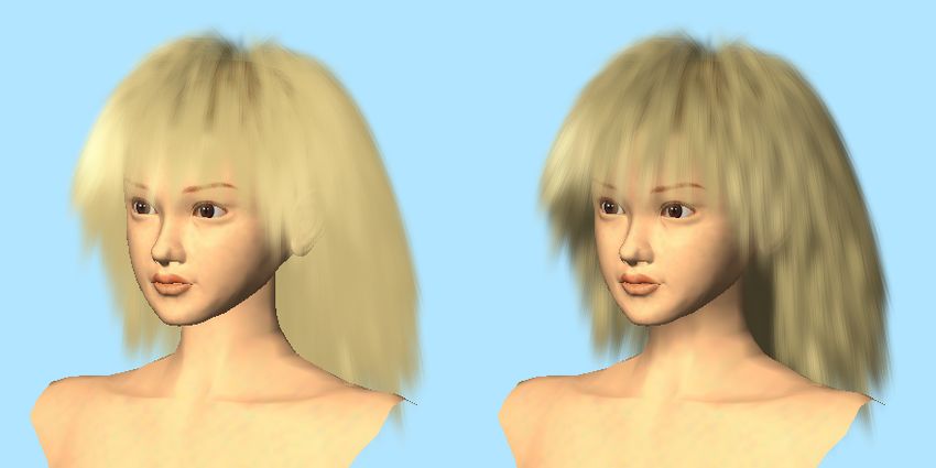
Bando, Chen, and Nishita / Animating Hair with Loosely Connected Particles

                                              v                                                                              xi

                                          1
                                                                                                                lij          θij                                   ti
                                                                                                                                   ti
                                                                                                  2h1                  xij              xi                         t ij
                                                                                          i
                                                                                                                                                                   θij

                                                                                                                                             rotatio
                                                                                           ti                                                                xij
                                                                      u                                   xj          θji
                                          0                     1                                                                                                         xj

                                                                                                                                                    n axis
                                                                                                               tj
                    (a)                                (b)
                                                                                         (a)                        (b)                                 (c)
        s

                   L(u, v)
                                                                                Figure 3: (a) The neighbor search is performed with a
                                                                                smoothing length h1 (so the radius is set as 2h1 ), and the
                                                                                particles connected with the center particle i are divided
                    v                                                           into two groups: Nr (i) (the blue nodes) and Nt (i) (the green
                                                                                nodes). (b) The initial state of a particle pair. (c) A diagram
             1
                                                                                for updating the hair direction.
   0
                                   u
                          1
  -sr
            lower bound
                                                                                computational efficiency, we first omit the pairs which have
                    (c)                                (d)                      ai j smaller than a threshold a0 . Then, from the pairs which
Figure 2: Initializing particles over the scalp. (a) A trimmed                  have smaller values for ci jW (li j , h1 ), which is the initial
scalp surface. (b) The scalp surface embedded in a unit                         spring coefficient between the two particles as will be de-
square. (c) The volume of the parameter domain (u, v, s). (d)                   scribed in Equation (7) in the next subsection, we omit them
The particles mapped back to the world space. The line seg-                     recursively until the number of connections for each parti-
ments indicate the hair directions.                                             cle is around the specified value Nn . Experimentally we use
                                                                                a0 = 0.5 and Nn = 12. In Figure 3 (a), Nn = 6.

above procedure, where h1 is a little larger than the initial                   3.3. Dynamics of Hair
average inter-particle distance. Moreover, we store the initial                 In this subsection, we focus on the dynamics of hair that is
state of each particle pair (i, j) by computing the distance li j               due to the characteristics of hair strands, and hair-hair inter-
between the two particles, and the angle θi j between the hair                  actions are explained in the next subsection.
direction ti and the direction of the particle pair xi j = x j −xi ,
as shown in Figure 3 (b).                                                          The hair volume can be considered as a deformable body,
                                                                                which can be animated by connecting the neighboring parti-
   We assign a strength of connection ci j to the particle pair                 cles with damped springs. The particle pairs are established
using the following equation, which is used for the spring                      using smoothing length h1 in the initialization process de-
coefficients described in the next subsection:                                  scribed in the previous subsection and this set of pairs is
                              c i j = a i j li j ,                        (5)   fixed during the animation phase. Since the hair volume
                                                                                deforms anisotropically, i.e., it is hard to stretch but free
where ai j indicates the degree               to which two particles are        to move laterally as Chang et al.4 pointed out, we model
aligned in a row and thus how                 strong their lengthwise co-       large tensile stiffness and small bending stiffness of the hair,
herence is. This is defined as:                                                 though we do not consider the twist of hair and neglect the
           | cos θi j − cos θ ji |/2           cos θi j · cos θ ji < 0          torsional stiffness. To realize free lateral motion of the hair,

  ai j =                                                               , (6)
           0                                   otherwise                        we make the connections between the particles loose by us-
                                                                                ing the following spring coefficient, which is a function of
which has the maximum value of 1 when the three vectors
                                                                                the current distance between a pair of particles:
ti , t j and xi j are oriented in the same direction. Even when
ti and t j are colinear, the two particles are not considered                                       ki j = ci jW (||xi j ||, h1 ),                                        (7)
to be well aligned if xi j is perpendicular to them. Because
                                                                                which gradually decreases as the two particles draw apart
we activate the spring forces that account for the stiffness
                                                                                until they become free from each other at a distance of 2h1 .
of the hair strands, connecting particles in close proximity
with stiff springs makes the system unstable. Therefore, the                       However, these loose connections also allow the hair to
second factor li j in Equation (5) is used for stability. For                   stretch. Therefore, in order to prevent the tensile stiffness of

                                                                                                 c The Eurographics Association and Blackwell Publishers 2006.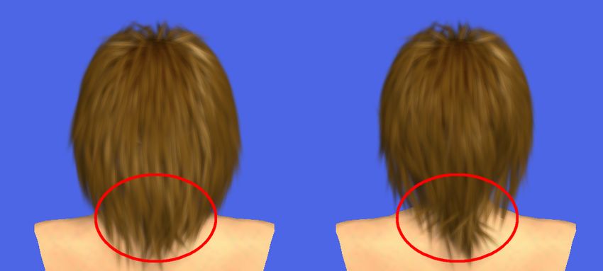
Bando, Chen, and Nishita / Animating Hair with Loosely Connected Particles

hair from changing, we keep the tensile elastic modulus of                        In summary, at each time step, we first compute the raw
each particle constant during animation. The elastic modulus                   spring coefficients ki j using Equation (7), then we com-
(also known as Young’s modulus) E is unique to a material,                     pute the scaling factors αi j using Equations (13) and (14),
and we can relate it to the rest length L and a cross-sectional                and finally we activate spring forces with spring coefficients
area A of the material by the following equation:                              αi j ki j . As the particles draw apart and several connections
                                L                                              between them become weak or have no effect, the remaining
                                  E=
                                   K,                       (8)                connections become strong to maintain the tensile stiffness.
                                A
                                                                               Even though the particles have no direct connections to the
where K corresponds to the spring coefficient when we view
                                                                               scalp, the hair neither stretches nor comes apart.
the material as the lengthwise spring. In the following, we
express E in terms of the parameters of the particles and the                     Based on the current spring coefficient αi j ki j , we update
springs connected between them. The cross-sectional area Ai                    the hair direction ti of particle i. As described in Section 3.2,
of the hair which particle i represents (not of individual hair                particle i has the initial angle θi j between the hair direction
strands) can be written as the following equation using the                    ti and the direction of the connection xi j . Thus, we can com-
density δ of the hair material:                                                                                     j
                                                                               pute the updated hair direction ti by rotating the normalized
                              m 2
                                  i 3                                          vector of xi j by angle θi j around the axis normal to both ti
                        Ai =          .                     (9)                and xi j , as shown in Figure 3 (c). Taking the weighted sum,
                                 δ
                                                                               the final updated hair direction is:
   Since we are concerned with the tensile stiffness of the
                                                                                                         t∗i = ∑ αi j ki j ti ,
                                                                                                                             j
hair, we divide the neighboring particles of particle i into two                                                                                  (15)
groups, as shown in Figure 3 (a): one includes those closer to                                                    j
the root of the hair, and the other includes those closer to the               where t∗i is subsequently normalized.
tip of the hair. They are denoted by Nr (i) and Nt (i), respec-
tively. For each group, we sum up all of the contributions of
the springs to the elastic modulus of particle i, which is kept                3.4. Hair-hair Interactions
constant by solving the following equations with unknown
scaling factors αi j for the spring coefficients ki j :                        We model attraction/repulsion, collision, and friction to ac-
                                                                               count for hair-hair interactions. The forces due to these inter-
                                 1
                       E =
                                 Ai     ∑        li j α i j k i j     (10)     actions act upon current nearby particles, and can be mod-
                                                                               eled by using a smoothing length h2 that is a little smaller
                                      j∈Nr (i)
                                 1                                             than the initial average inter-particle distance.
                       E =
                                 Ai     ∑        li j α i j k i j ,   (11)
                                                                                  Attraction/repulsion forces can be caused by lipids, hair-
                                      j∈Nt (i)
                                                                               dressings or static electricity. Macroscopically, the effect of
where li j is the rest length of the spring between particles i
                                                                               these interactions is to preserve the average density of hair.
and j, which is their initial distance as described in Section
                                                                               The force on particle i due to particle j is given by the fol-
3.2. The number of unknowns αi j is the number of particle
                                                                               lowing equation, which is the pressure force in SPH18 :
pairs, and it is much larger than the number of equations,
which is twice the number of particles. Thus, Equations (10)
                                                                                                                !
                                                                                                       Pi    Pj    ∂
and (11) form an underdetermined sparse linear system. To                           fa, ji = −mi m j      + 2        W (||xi j ||, h2 ), (16)
                                                                                                      ρ2i    ρ j ∂xi
keep the computational cost as low as possible, we directly
(non-iteratively) obtain an approximate solution to this sys-                  where the pressure P is modeled as P = ka (ρ − ρ0 ) and ka
tem in linear time in the number of particles, which cannot                    and ρ0 control the magnitude of the force and the average
be accomplished by the least square methods for underde-                       density, respectively6 . A small value for ρ0 makes the hair
termined linear systems5 . Since the spring coefficients ki j                  repulsive, whereas a large value makes it cohesive.
already include weighting factors through Equation (7), we
                                                                                    To model inelastic collisions of hair, we simply reduce
make αi j independent of j as:
                                                                               the relative velocity vi j = v j − vi of two particles if they are
                      αi j = αr,i for ∀ j ∈ Nr (i),                   (12)     approaching. The direction of the collision, dn , is normal to
and we solve Equation (10) for each i individually:                            the hair directions ti and t j of both particles. Thus, dn = ti ×
                                                                               t j . If ||dn ||  1, the two hair directions are almost colinear,
                                         EAi                                   and in this case we can compute the direction of the collision
                           αr,i =                    .                (13)
                                        ∑ li j k i j                           as dn = xi j − (xi j · ti )ti . After normalizing dn , we check the
                                      j∈Nr (i)
                                                                               sign of (xi j · dn )(vi j · dn ). If this is negative, the two particles
Similarly Equation (11) is solved to obtain αt,i , and we take                 are approaching, and we apply the following force:
the average of the two solutions as follows:
                                                                                             fc, ji = dc W (||xi j ||, h2 ) (vi j · dn )dn ,      (17)
            (αr,i + αt, j )/2 i ∈ Nt ( j) ∧ j ∈ Nr (i)

   αi j =                                              . (14)
            (αr, j + αt,i )/2 i ∈ Nr ( j) ∧ j ∈ Nt (i)                         where dc is the collision damping constant.

c The Eurographics Association and Blackwell Publishers 2006.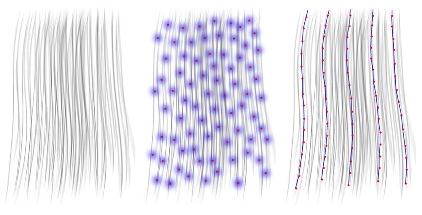
Bando, Chen, and Nishita / Animating Hair with Loosely Connected Particles

   Friction is modeled similarly. The direction dt of the fric-
tional force is defined as vi j − (vi j · dn )dn , which is normal
to the direction of the collision dn . After normalizing it, the
force is computed as:
             f f , ji = d f W (||xi j ||, h2 ) (vi j · dt )dt ,   (18)
where d f is the frictional damping constant.

3.5. Other Forces
We model gravity, air friction, wind, inertia due to head                                  (a)                                    (b)
movement, and collisions against the body (the head and the                  Figure 4: The hair rendered (a) without (b) with shadows.
torso). Gravity is a downward force whose magnitude is pro-
portional to the particle mass, and air friction is modeled as
a damping force whose magnitude is proportional to the par-
                                                                               To simulate the highly anisotropic phase function of hair
ticle velocity.
                                                                            we use the Goldman model9 , which adds a directionality fac-
   The wind is also represented by a set of particles, and is               tor to the Kajiya-Kay model11 that controls the reflection
simulated using SPH18 . The interactions between the hair                   and transmission ratios of light. However, as the number of
particles and the air particles are modeled as drag forces be-              particles is relatively small for computational efficiency, the
tween them10 , and thus the wind is also affected by move-                  phase function alone is not sufficient to produce the appear-
ment of the hair. Though these interactions include the effect              ance of hair strands. We compensate this loss by mapping
of air friction, the damping force described above is still nec-            hair texture to the billboards instead of the simple texture of
essary to prevent abrupt motion of the hair. Since our LCP                  a Gaussian distribution. Figure 5 (a) shows an example of
approach models hair solely with particles, other particle-                 hair texture. We match the hair direction of the texture (usu-
based methods are easily incorporated with a slight modifi-                 ally the vertical axis) to the particle direction ti as shown
cation to the programming code.                                             in Figure 5 (b). As opposed to the standard billboard, we
   The reason to model inertia is that it is numerically more               can only place it so that its horizontal axis is parallel to
stable to modify the particle accelerations than their posi-                the screen. Hence, we scale the opacity of the billboard by
tions. We describe the equations of motion of the particles                 1/ sin θ, where cos θ = ti · d p and d p is the direction of pro-
with respect to the local coordinate system attached to the                 jection. We can further augment the directionality by scaling
head, and we exert inertial forces on the particles, avoiding               the size of the billboards as shown in Figure 5 (c).
directly altering their positions relative to the head.
                                                                                                    standard billboard
   After applying all of the forces described so far, collisions
between the particles and the body are detected efficiently by                                                            our billboard
again utilizing the voxel grid structure. And each particle in                                                                   ti              ti
contact with the body suffers a repulsive force that dissipates
its relative velocity normal to the body, and a frictional force
                                                                                                   scr
is also exerted according to Coulomb’s model2 .                                                       een                  dp

4. Rendering Hair                                                                   (a)                      (b)                           (c)

Since the particles represent the volume density of hair, we                Figure 5: (a) An example of hair texture. (b) The hair direc-
can render hair by using volume rendering techniques, just                  tion of the texture is matched to the particle direction. This
as Kajiya and Kay did for their furry teddy bear11 . Unlike the             figure shows the case of orthogonal projection. The case of
standard voxel grid structure, the density field in our model               perspective projection is similar. (c) The size of the billboard
is represented by the distribution of particles, and in this case           is scaled.
we can benefit greatly from the splatting method with bill-
boards by using the hardware accelerated method presented
by Dobashi et al.7 . We assume a parallel light source, and in
                                                                            5. Results
the first pass, we project the particles in the direction of the
light source in order to ascertain how much of the light in-                We successfully animated the hair with a head and torso
tensity is attenuated. In the second pass, we can then render               model at an interactive frame rate. Figures 6 (a) – (c) show a
the hair with complex self-shadows that enhance the volu-                   few frames from an animation of back hair. The hair is forced
metric appearance of the hair. Figure 4 shows the rendered                  to split into two, and then merges again because of grav-
images of our hair model without and with shadows.                          ity. Hair-hair interactions prevent the hairs from penetrating

                                                                                             c The Eurographics Association and Blackwell Publishers 2006.
Bando, Chen, and Nishita / Animating Hair with Loosely Connected Particles
each other as shown in Figure 6 (c), which is a contrast to
Figure 6 (d) where hair-hair interactions are not considered.
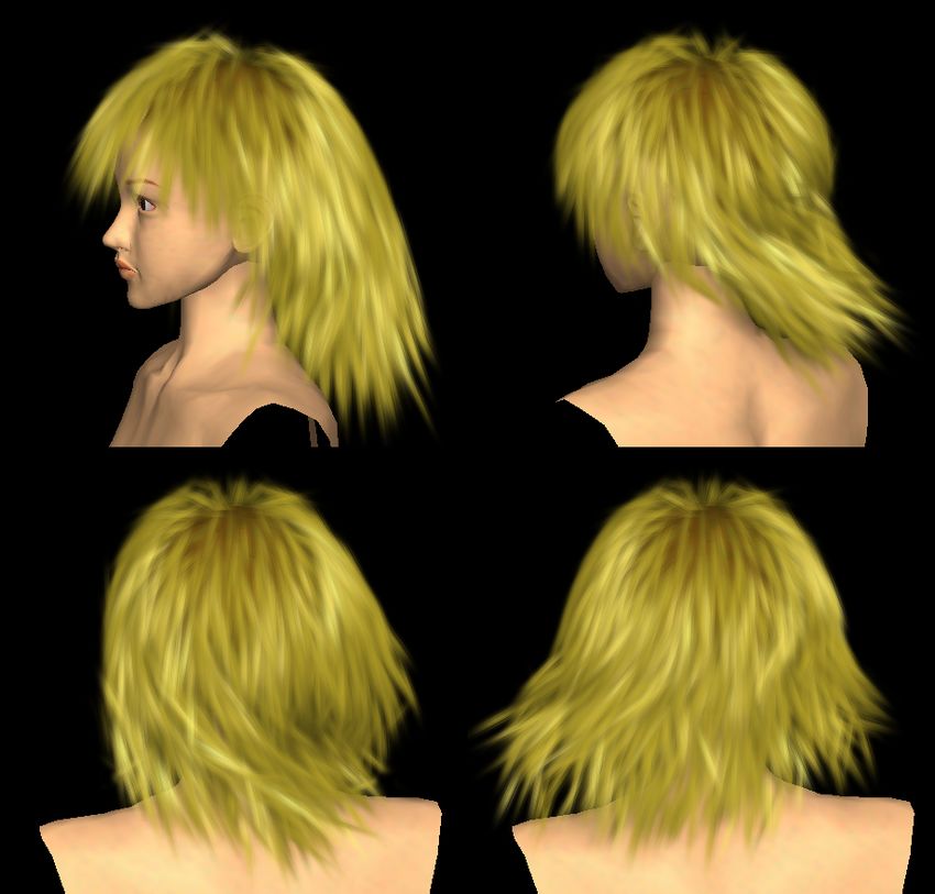
Figure 7 shows an animation of hair when the head is shaken.
The head turns around and the hair follows this motion with
delay because of inertia. Dynamic clustering effects are vis-
ible. Figure 8 shows an animation of hair blowing in wind.
Interactions between the hair and the air are also simulated.
(a) (b)
Figure 8: Animation of hair blowing in wind. Left to right,
top to bottom.
We used about 2,000 particles to represent the hair for
all of the animations presented above. The number of parti-
(c) (d) cles is determined by a compromise between accuracy and
efficiency, and we chose the number so that the animation,
Figure 6: (a) – (c) A few frames from an animation of back including both simulation and rendering with shadows, can
hair. (d) The hairs penetrate each other when hair-hair in- be performed at an interactive frame rate. The hair was ani-
teractions are not considered, which is a contrast to (c). The mated at 6.7 fps on a PC with an Intel Pentium 4 2.8 GHz
difference is clearly seen in the red circles. CPU and an NVIDIA Quadro4 900 XGL GPU. The simu-
lation took 33% of the total computation time, and the ren-
dering took the rest. The size of the image and the buffer for
computing shadows is 512 × 512.
6. Conclusions and Future Work
This paper has presented a practical method for animating
hair with a new model called loosely connected particles
(LCP). The hair is modeled as a set of unordered particles
that serve as sampling points for the volume of the hair. The
loose connections between the particles make the hair free to
move laterally, nevertheless providing lengthwise coherence
by maintaining their tensile stiffness. The hair is rendered
by placing billboards with hair texture at the positions of the
particles, utilizing graphics hardware accelerations.
Our LCP approach has the following advantages:
• It reduces the high computational cost of simulating the
dynamics of the hair including hair-hair interactions, and
realizes interactive hair animation.
• The simulation is solely based on the particle dynamics,
Figure 7: Animation of hair when the head is shaken. Left to which simplifies the implementation. Other particle-based
right, top to bottom. methods can be easily incorporated.
On the other hand, there are limitations to our method:
c The Eurographics Association and Blackwell Publishers 2006.Bando, Chen, and Nishita / Animating Hair with Loosely Connected Particles
• It is applicable to only a simple hairstyle, and extension to 8. M. Eck, T. DeRose, T. Duchamp, H. Hoppe, M. Louns-
various hairstyles is a major remaining task. bery, and W. Stuetzle. Multiresolution analysis of ar-
• The simulation is not physically rigorous. The nonlinear bitrary meshes. Proceedings of ACM SIGGRAPH ’95,
spring forces accounting for the stiffness of the hair are 173–182, 1995. 3
designed to obtain the desirable motion of the hair, and
9. D. Goldman. Fake fur rendering. Proceedings of ACM
the bending stiffness is not modeled explicitly.
SIGGRAPH ’97, 127–134, 1997. 6
• The hair is still rendered coarsely. Interpolating between
the particles to place many smaller billboards would pro- 10. S. Hadap and N. Magnenat-Thalmann. Modeling dy-
duce finer images, but this will slow down the system be- namic hair as a continuum. Computer Graphics Forum
low an interactive frame rate on current computers. (Eurographics 2001 Proc.), 20(3):329–338, 2001. 1,
2, 6
In addition to addressing the above limitations, the future
direction of this work would be to take further advantage of 11. J. Kajiya and T. Kay. Rendering fur with three di-
the particle representation, for example, adaptive sampling mensional textures. ACM Computer Graphics (Proc.
of the hair volume and incorporating the simulation level of of SIGGRAPH ’89), 23(4):271–280, 1989. 6
detail technique19 . 12. T.-Y. Kim. Modeling, Rendering and Animating Hu-
man Hair. Ph.D dissertation, University of Southern
Acknowledgments California, 2002. 2
We thank Prof. Nelson Max (University of California) and 13. T.-Y. Kim and U. Neumann. A thin shell volume for
Dr. Yoshinori Dobashi (Hokkaido University) for many use- modeling human hair. Proceedings of Computer Ani-
ful suggestions, and Ryoichi Mizuno for naming our hair mation 2000, 121–128, 2000. 1, 2
model “loosely connected particles.” This project is partially 14. T.-Y. Kim and U. Neumann. Interactive multiresolu-
supported by Toshiba Corporation. tion hair modeling and editing. ACM Transactions on
Graphics (Proc. of SIGGRAPH 2002), 21(3):620–629,
References 2002. 2
1. K. Anjyo, Y. Usami, and T. Kurihara. A simple method 15. C. K. Koh and Z. Huang. A simple physics model to
for extracting the natural beauty of hair. ACM Com- animate human hair modeled in 2D strips in real time.
puter Graphics (Proc. of SIGGRAPH ’92), 26(2):111– Proceedings of Eurographics Workshop on Computer
120, 1992. 3 Animation and Simulation 2001, 127–138, 2001. 2
2. R. Bridson, R. Fedkiw, and J. Anderson. Robust treat- 16. D.-W. Lee and H.-S. Ko. Natural hairstyle modeling
ment of collisions, contact and friction for cloth ani- and animation. Graphical Models, 63(2):67–85, 2001.
mation. ACM Transactions on Graphics (Proc. of SIG- 1, 2
GRAPH 2002), 21(3):594–603, 2002. 6 17. N. Magnenat-Thalmann, S. Hadap, and P. Kalra. State
3. E. Catmull and R. Rom. A class of local interpolating of the art in hair simulation. Proceedings of Interna-
splines. Computer Aided Geometric Design (Proc. of tional Workshop on Human Modeling and Animation
International Conference on Computer Aided Geomet- 2000, 3–9, 2000. 2
ric Design ’74), 317–326, 1974. 3 18. J. J. Monaghan. Smoothed particle hydrodynamics. An-
4. J. T. Chang, J. Jin, and Y. Yu. A practical model for nual Review of Astronomy and Astrophysics, 30:543–
hair mutual interactions. Proceedings of ACM SIG- 574, 1992. 2, 3, 5, 6
GRAPH Symposium on Computer Animation 2002, 73– 19. D. O’Brien, S. Fisher, and M. C. Lin. Automatic sim-
80, 2002. 1, 2, 4 plification of particle system dynamics. Proceedings of
Computer Animation 2001, 210–219, 2001. 8
5. R. E. Cline and R. J. Plemmons. l2 -solutions to un-
derdetermined linear systems. SIAM Review, 18(1):92– 20. E. Plante, M.-P. Cani, and P. Poulin. A layered wisp
106, 1976. 5 model for simulating interactions inside long hair. Pro-
ceedings of Eurographics Workshop on Computer Ani-
6. M. Desbrun and M.-P. Gascuel. Smoothed particles: a
mation and Simulation 2001, 139–148, 2001. 1, 2
new paradigm for animating highly deformable bodies.
Proceedings of Eurographics Workshop on Computer 21. C. R. Robbins. Chemical and Physical Behavior of Hu-
Animation and Simulation ’96, 61–76, 1996. 2, 3, 5 man Hair (4th ed.). Springer-Verlag, 2002. 1
7. Y. Dobashi, K. Kaneda, H. Yamashita, T. Okita, and T. 22. R. Rosenblum, W. Carlson, and E. Tripp. Simulating
Nishita. A simple, efficient method for realistic anima- the structure and dynamics of human hair: modeling,
tion of clouds. Proceedings of ACM SIGGRAPH 2000, rendering and animation. The Journal of Visualization
19–28, 2000. 6 and Computer Animation, 2(4):141–148, 1991. 1
c The Eurographics Association and Blackwell Publishers 2006.You can also read