Contemporary wildfire hazard across California - PREPARED FOR: PREPARED BY: Pyrologix

contemporary
wildfire hazard
across California

PREPARED FOR:
Pacific Southwest Region, USDA Forest Service

PREPARED BY:
Kevin C. Vogler, April Brough,
Chris J. Moran, Joe H. Scott,
Julie W. Gilbertson-Day

June 30, 2021

Last updated: July 13, 2021

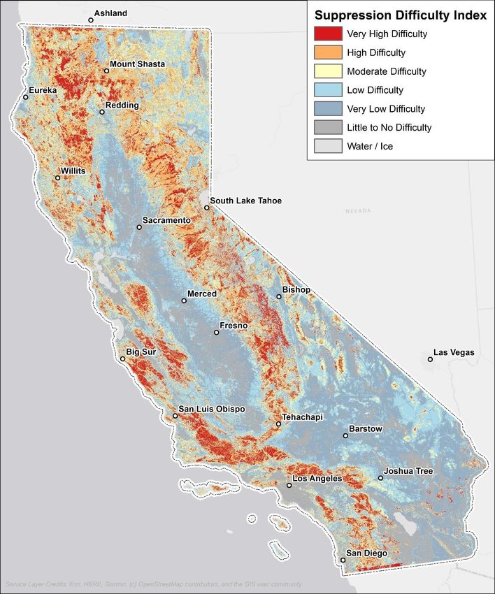
TABLE OF CONTENTS

1 Executive Summary ....................................................................................................................... 6
 1.1 Purpose of the Assessment .......................................................................................................................7
 1.2 Quantitative Risk Modeling Framework ..............................................................................................7

2 Wildfire Likelihood ........................................................................................................................ 8
 2.1 Overview of Methods ..................................................................................................................................8
 FSim ........................................................................................................................................................................ 8
 2.2 Landscape Zones ...........................................................................................................................................9
 Analysis Area ...................................................................................................................................................... 9
 Fire Occurrence Areas .................................................................................................................................. 9
 Fuelscape Extent ........................................................................................................................................... 10
 2.3 Analysis Methods and Input Data ........................................................................................................ 10
 Fuelscape .......................................................................................................................................................... 11
 Historical Wildfire Occurrence ............................................................................................................. 12
 Historical Weather....................................................................................................................................... 17
 Suppression Modeling ................................................................................................................................ 19
 2.4 Wildfire Simulation ................................................................................................................................... 19
 Model Calibration......................................................................................................................................... 20
 Integrating FOAs .......................................................................................................................................... 20
 2.5 Wildfire Modeling Results ...................................................................................................................... 20
 Upsampling FSim Results ......................................................................................................................... 21

3 Wildfire Behavior Characteristics .......................................................................................... 23
 3.1 Overview of methods ............................................................................................................................... 23
 FSim versus WildEST .................................................................................................................................. 23
 Weather Type Probability rasters ........................................................................................................ 25
 3.2 Flame front characteristics..................................................................................................................... 26
 Rate of Spread (ROS) .................................................................................................................................. 26
 Flame Length (FL) ......................................................................................................................................... 27
 Fire-Type probability (FTP) ..................................................................................................................... 27
 Probability of Operational Control ...................................................................................................... 28

 1

Headfire flame-length probabilities (Ops FLPs)............................................................................ 28
 “Fire-effects” flame-length probabilities ........................................................................................... 29
 3.3 Ember characteristics............................................................................................................................... 37
 Ember Production Index ........................................................................................................................... 37
 Ember Load Index ......................................................................................................................................... 37

4 Integrated Hazard ........................................................................................................................ 39
 4.1 Risk to Potential Structures (RPS) ....................................................................................................... 39
 4.2 Wildfire Hazard Potential (WHP) ........................................................................................................ 42
 4.3 Suppression Difficulty Index (SDI) ....................................................................................................... 44

5 Discussion ....................................................................................................................................... 46

6 References...................................................................................................................................... 47

7 Data Products................................................................................................................................ 49

8 Change Log ..................................................................................................................................... 52

 2

LIST OF TABLES
Table 1. Historical large-fire occurrence, 1992-2017, in the California FSim project FOAs............. 12

Table 2. Adjustments to calibration targets to account for trends in wildfire occurrence. ................ 16

Table 3. Fuel Moisture values used in wildfire simulation for the 80th/90th/97th percentile ERCs.. 18

Table 4. Burn minutes table for calculating area burned index (ABI). .................................................... 25

Table 5. The WildEST Type of Fire classification. ......................................................................................... 28

Table 6. Risk to Potential Structures response function by flame length class ...................................... 39

 3

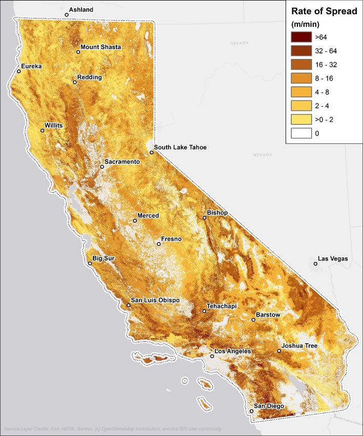
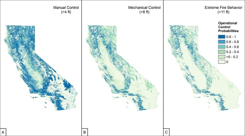
LIST OF FIGURES
Figure 1. The components of a Quantitative Wildfire Risk Assessment Framework..............................7

Figure 2 Overview of landscape zones for California State FSim project. ..................................................9

Figure 3. Diagram showing the primary elements used to derive burn probability.............................. 10

Figure 4. Map of fuel model groups across the California State LCP extent ........................................... 11

Figure 5. Shows the Ignition Density Grid for the California State Fire Occurrence Area. ............... 13

Figure 6. Historical Analysis Groups used in 2020 Trend Analysis. ........................................................... 14

Figure 7. Historical Wildfire Occurrence (1992 – 2017) in analysis Group 1. ........................................ 15

Figure 8. Historical Wildfire Occurrence (1992 – 2017) in analysis Group 2. ........................................ 15

Figure 9. Historical Wildfire Occurrence (1992 – 2017) in analysis Group 3 ......................................... 16

Figure 10. Sample points from the 2-km gridded hourly WRF dataset generated by DRI. ................ 17

Figure 11. Map of Direct Protection Area (DPA) for the California State analysis area. .................... 19

Figure 12. Map of integrated FSim burn probability results for the California study area at 30-m
 resolution. .............................................................................................................................................................. 22

Figure 13. Headfire flame-length probabilities (top) and non-heading (or “fire effects”) flame-length
 probabilities (bottom)........................................................................................................................................ 30

Figure 14. Map of WildEST 30-m Rate of Spread (m/min) for the CAL analysis area........................... 31

Figure 15. Map of WildEST 30-m Mean Flame Length (ft) for the CAL analysis area. ......................... 32

Figure 16. Map of WildEST 30-m Fire Type Probabilities for the CAL analysis area. These include
 (A) non-fuel, (B) surface, (C) underburn, (D) low-grade passive crown fire, (E) mid-grade passive
 crown fire, (F) high-grade passive crown fire, and (G) active crown fire. Probabilities range in
 value from 0 to 1, with (A) and (B) being binary rasters of only values 0 and 1. ............................ 33

Figure 17. Map of WildEST 30-m Operation Control Probabilities for the CAL analysis area. ........ 34

Figure 18. Map of WildEST 30-m heading FLPs for the CAL analysis area. Panels A-F show the FLP
 for the heading flame-length bin specified. The sum of A-F for any given pixel equals 1. ......... 35

Figure 19. Map of WildEST 30-m fire-effects FLPs for the CAL analysis area. A-F show the FLP for
 the fire-effects flame-length bin specified. The sum of A-F for any given pixel equals 1. .......... 36

Figure 20. Map of WildEST 30-m ember indices for the CAL analysis area. These include (A)
 conditional Ember Production Index, (B) Ember Production Index, (C) conditional Ember Load
 Index, and (D) Ember Load Index. Probabilities range in value from 0 to 1. ................................... 38

 4

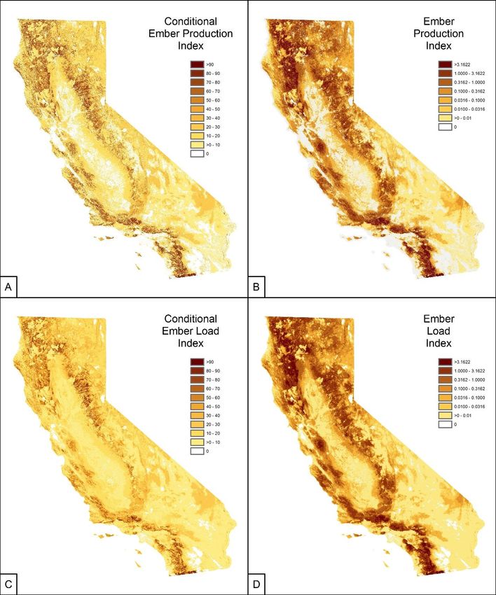
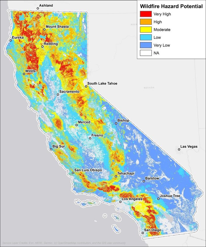
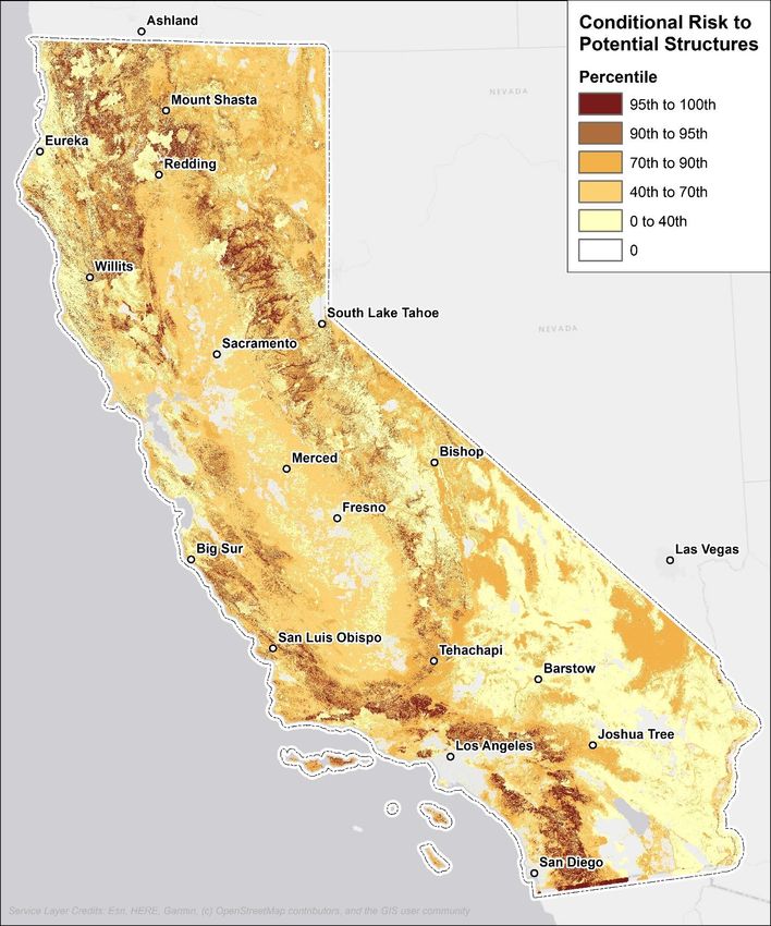
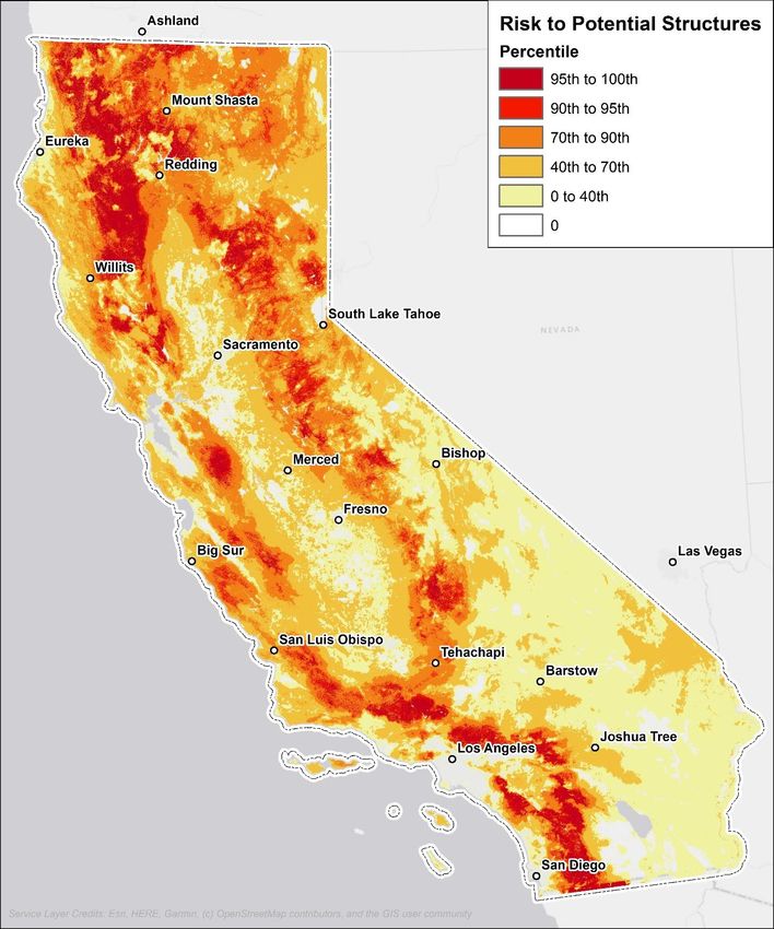
Figure 21. Map of 30-m conditional Risk to Potential Structures for the CAL analysis area. ........... 40

Figure 22. Map of 30-m Risk to Potential Structures for the CAL analysis area. ................................... 41

Figure 23. Map of 30-m Wildfire Hazard Potential for CAL analysis area. .............................................. 43

Figure 24. Map of 30-m Suppression Difficulty Index for CAL analysis area. ......................................... 45

 5

1 Executive Summary
 In July 2019, the Pacific Southwest Region of the U.S. Forest Service contracted with Pyrologix to
 conduct a spatial wildfire hazard assessment across all land ownerships across the state of
 California. The project consisted of three parts: fuelscape calibration, wildfire hazard assessment,
 and summary of wildfire risk to California communities.
 In early March 2020, just days before nationwide shutdowns due to Covid-19, Pyrologix led two in-
 person fuel calibration workshops hosted by the Region and attended by a wide array of local, state,
 and federal specialists in the fields of fuel characterization, fire ecology, and fire behavior modeling.
 By mid-summer 2020 Pyrologix produced a 2020 fuelscape. A report describing the methods used
 to produce the fuelscape is available for download here1.
 In the summer and fall of 2020, Pyrologix used spatial datasets of historical weather and fire
 occurrence to parameterize and calibrate a comprehensive USFS fire modeling system called FSim
 to estimate annual burn probability across California. FSim also produced an “event set” that was
 later used to estimate transmission of fire damage to homes—from the origin locations of simulated
 wildfires to where their damage occurred. During this time, Pyrologix also applied a comprehensive
 simulation of potential wildfire behavior characteristics based on FlamMap, another US Forest
 Service fire modeling system.
 These simulations of wildfire hazard (likelihood and intensity) were used to calculate indices of
 integrated hazard, including Risk to Potential Structures, Suppression Difficulty Index, and Wildfire
 Hazard Potential. Pyrologix used several of the assessment results, in conjunction with a housing-
 unit density dataset (called HUDen2), to summarize wildfire risk to homes across California. Risk to
 homes was summarized for counties, county divisions, ZIP codes, and Census Populated Places and
 presented in a separate report entitled “Wildfire Risk to California Communities”3.
 This report documents the wildfire hazard simulation portion of the project and represents the best
 available science across a range of disciplines. While this report was generated by Pyrologix LLC,
 the overall analysis was developed as a collaborative effort with numerous agencies and partners
 providing data and feedback.
 The results produced in this analysis provide a snapshot of wildfire hazard conditions before the
 2020 fire season. Following the historic 2020 fire season in California, an update to these results is
 needed and is already underway. Additionally, a separate expanded effort to assess wildfire risk to
 homes, critical infrastructure, and surface drinking water is also underway.

 1
 CAL Fuelscape report: http://pyrologix.com/wp-content/uploads/2021/06/CAL_FuelscapeReport.pdf
 2
 HuDEN was produced for the Wildfire Risk to Communities project (wildfirerisk.org) and is available for
 download here: https://www.fs.usda.gov/rds/archive/catalog/RDS-2020-0060
 3
 http://pyrologix.com/reports/Wildfire-Risk-to-California-Communities.pdf

 6

1.1 PURPOSE OF THE ASSESSMENT
The purpose of the California State Quantitative Wildfire Hazard Assessment report is to provide
foundational information about wildfire hazard across the geographic area. Such information
supports wildfire response, regional fuel management planning decisions, and revisions to land and
resource management plans. The California State analysis considers:
 • likelihood of a fire burning

 • the intensity of a fire if one should occur.

To manage wildfire in California, it is essential that accurate wildfire hazard data, to the greatest
degree possible, is available to drive fire management strategies. These hazard outputs can be used
to inform the planning, prioritization, and implementation of prevention and mitigation activities,
such as prescribed fire and mechanical fuel treatments. In addition, the hazard data can be used to
support fire operations and aid in decision-making for the allocation and positioning of firefighting
resources.

1.2 QUANTITATIVE RISK MODELING FRAMEWORK
The basis for a quantitative framework for assessing wildfire risk to highly valued resources and
assets (HVRAs) has been established for many years (Finney, 2005; Scott, 2006). The framework
has been implemented across a range of scales, from an individual county (Ager, 2017), a portion of
a national forest (Thompson et al., 2013a), individual states (Buckley et al., 2014), to the entire
continental United States (Calkin et al., 2010). In this framework, wildfire risk is a function of two
main factors: 1) wildfire hazard and 2) HVRA vulnerability (Figure 1).

Figure 1. The components of a Quantitative Wildfire Risk Assessment Framework.

 7

Wildfire hazard is a physical situation with the potential for causing damage to vulnerable
 resources or assets. Quantitatively, wildfire hazard is measured by two main factors: 1) burn
 probability (or likelihood of burning), and 2) fire intensity (measured as flame length, fireline
 intensity, or other similar measures).
 HVRA vulnerability is also composed of two factors: 1) exposure and 2) susceptibility. Exposure is
 the placement (or coincidental location) of an HVRA in a hazardous environment—for example,
 building a home within a flammable landscape. Some HVRAs, like wildlife habitat or vegetation
 types, are not movable; they are not "placed" in hazardous locations. Still, their exposure to wildfire
 is the wildfire hazard where the habitat exists. Finally, the susceptibility of an HVRA to wildfire is
 how easily it is damaged by wildfire of different types and intensities. Some assets are fire-hardened
 and can withstand very intense fires without damage, whereas others are easily damaged by even
 low-intensity fire.
 This report will describe the data and methods used in developing estimates of wildfire probability
 and intensity for the California State analysis area.

2 Wildfire Likelihood

 2.1 OVERVIEW OF METHODS

 FSIM
 The FSim large-fire simulator was used to quantify wildfire likelihood across the Analysis Area at a
 pixel size of 120 meters. FSim is a comprehensive fire occurrence, growth, behavior, and
 suppression simulation system that uses locally relevant fuel, weather, topography, and historical
 fire occurrence information to make a spatially resolved estimate of the contemporary likelihood
 and intensity of wildfire across the landscape (Finney et al., 2011).
 FSim focuses on the relatively small fraction of wildfires that escape initial attack and become
 "large" (>247.1 acres). Since the occurrence of large fires is relatively rare, FSim generates many
 thousands of years of simulations, to capture a sample size large enough to generate burn
 probabilities for the entire landscape. An FSim iteration spans one entire year. All Fire Occurrence
 Areas (FOAs) within the California project area were run with 10,000 iterations.
 There is no temporal component to FSim beyond a single wildfire season, consisting of up to 365
 days. FSim performs independent (and varying) iterations of one year, defined by the fuel, weather,
 topography, and wildfire occurrence inputs provided. FSim does not account for how a simulated
 wildfire might influence the likelihood or intensity of future wildfires (even within the same
 simulation year). Each year represents an independent realization of how fires might burn given the
 current fuelscape and historical weather conditions. FSim integrates all simulated iterations into a
 probabilistic result of wildfire likelihood.
 In addition to estimates of wildfire likelihood, FSim produces measurements of predicted wildfire
 intensities. There are however inherent challenges of estimating intensity with a stochastic
 simulator. Estimates of wildfire intensity were instead developed using a custom Pyrologix utility

 8

called WildEST (Scott, 2020). WildEST is a deterministic wildfire modeling tool that integrates
variable weather input variables and weights them based on how they will likely be realized on the
landscape. WildEST is more robust than the stochastic intensity values developed with FSim. This
is especially true in low wildfire occurrence areas where predicted intensity values from FSim are
reliant on a very small sample size of potential weather variables. The WildEST methodology is
further described in Section 3.

2.2 LANDSCAPE ZONES
Project boundaries for the California State wildfire hazard assessment were developed to not
introduce artificial seamlines during simulation modeling. The developed project boundaries that
were used in the FSim modeling are described below in sections 2.2.1- 2.2.3 and can be seen in
Figure 2.

 ANALYSIS AREA
The Analysis Area is the area for
which valid burn probability results
are produced. The Analysis Area for
the California project was defined
as the California state boundary
with a 10-kilometer buffer of
adjacent lands within the United
States.

 FIRE OCCURRENCE
AREAS
To ensure valid BP results in the
Analysis Area and prevent edge
effects, it is necessary to allow FSim
to start fires outside of the Analysis
Area and burn into it. This larger
area where simulated fires are
started is called the Fire Occurrence
Area (FOA). We established the
FOA extent as a 30-km buffer on the
Analysis Area including a 30-km
buffer beyond the U.S. border and
 Figure 2 Overview of landscape zones for California State FSim project.
into Mexico. The buffer provides
sufficient area to ensure all fires that could reach the Analysis Area are simulated. The Fire
Occurrence Area covers roughly 124.1 million acres and is characterized by diverse topographic
and vegetation conditions. We divided the overall fire occurrence area into fourteen FOAs to model
this large area where historical fire occurrence and fire weather are highly variable. Individual FOA
boundaries were developed to group geographic areas that experience similar wildfire occurrence.

 9

These boundaries were generated using a variety of inputs including larger fire occurrence
boundaries developed for national-level work (Short, 2020), aggregated level IV EPA Ecoregions,
and local fire staff input. For consistency with other FSim projects, we numbered these FOAs 510
through 523.

 FUELSCAPE EXTENT
The available fuelscape extent was determined by adding a 30-km buffer to the FOA extent. This
buffer allows fires starting within the FOA to grow unhindered by the edge of the fuelscape, which
would otherwise truncate fire growth and affect the simulated fire-size distribution and potentially
introduce errors in the calibration process. A map of the Analysis Area, FOA boundaries, and
fuelscape extent are presented in Figure 2.

2.3 ANALYSIS METHODS AND INPUT DATA
FSim is a comprehensive fire occurrence, growth, behavior, and suppression simulation system that
uses locally relevant fuel, weather, topography, and historical fire occurrence information to make
a spatially resolved estimate of the contemporary likelihood of wildfire across the landscape. Figure
3 below provides a graphical description of the various FSim inputs that are further discussed in
Sections 2.3.1 - 2.3.4.

Figure 3. Diagram showing the primary elements used to derive burn probability

 10

FUELSCAPE
The Pacific Southwest Region of the
USDA Forest Service contracted
Pyrologix to complete an
assessment of wildfire hazard
across all land ownerships in the
state of California. The foundation
of any wildfire hazard assessment is
a current-condition fuelscape,
updated for recent disturbances
and calibrated to reflect the fire
behavior potential realized in
recent historical wildfire events.
LANDFIRE 2016 Remap 2.0.0 (LF
Remap) data was leveraged to
generate a calibrated fuelscape for
use in this statewide assessment.
The fuelscape consists of geospatial
datasets representing surface fuel
model (FM40), canopy cover (CC),
canopy height (CH), canopy bulk
density (CBD), canopy base height
(CBH), and topography
characteristics (slope, aspect,
elevation). The FM40 dataset can be Figure 4. Map of fuel model groups across the California State LCP extent.
seen in Figure 4. The fuelscape datasets can be combined into a single landscape (LCP) file and used
as a fuelscape input in fire modeling programs.
The LANDFIRE 2016 Remap 2.0.0 base data was edited to remove mapping zone seamlines,
calibrated based on expert opinion at two fuel calibration workshops, and updated to represent the
most recent fuel disturbances through the end of 2019. Further details about the methods and base
data used to generate the calibrated California all lands fuelscape are available in the fuelscape
report1.

 11

HISTORICAL WILDFIRE OCCURRENCE
The Fire Occurrence Database (FOD) that spans the 26 years from 1992-2017 was used to quantify
historical large-fire occurrence (Short, 2017). Historical wildfire occurrence data were used to
develop model inputs (the fire-day distribution file [FDist] and ignition density grid [IDG]) as well as
model calibration targets. Table 1 summarizes the annual number of large fires per million acres,
mean large-fire size, and annual area burned by large fires per million acres for each FOA. For this
analysis, we defined a large fire as one greater than 247.1 acres (100 hectares).

Table 1. Historical large-fire occurrence, 1992-2017, in the California FSim project FOAs.
 Mean annual Mean annual
 Mean annual number of large-fire FOA-mean
 number of FOA area large fires Mean large- area burned burn
 FOA large fires (M ac) per M ac fire size (ac) (ac) probability
 510 2.96 5.39 0.55 3,513 10,403 0.0019
 511 9.58 7.78 1.23 11,249 107,731 0.0138

 512 7.08 9.25 0.76 5,971 42,253 0.0046

 513 2.12 3.43 0.62 4,214 8,915 0.0026
 514 5.58 4.91 1.14 5,432 30,296 0.0062

 515 6.62 2.88 2.30 3,548 23,472 0.0082

 516 12.31 9.32 1.32 5,827 71,713 0.0077
 517 10.04 10.97 0.92 1,173 11,776 0.0011

 519 13.50 11.51 1.17 5,263 71,056 0.0062

 520 5.54 1.87 2.96 1,536 8,507 0.0045

 521 9.77 6.57 1.49 4,321 42,208 0.0064
 522 7.35 27.64 0.27 2,769 20,338 0.0007

 523 3.27 11.45 0.32 1,419 4,640 0.0005

Historical wildfire occurrence varied substantially by FOA (Table 1), with FOA 519 experiencing
the highest annual average of 2.96 large wildfires per million acres. FOA 521 had the least frequent
rate of occurrence with an annual average of 0.27 large wildfires per million acres. FOA 511 has the
largest mean large-fire size of 11,249 acres while FOA 517 had the smallest with 1,173 acres.

 12

IGNITION DENSITY GRID
To account for the spatial variability
in historical wildfire occurrence
across the landscape, FSim uses a
geospatial layer representing the
relative, large-fire ignition density.
FSim stochastically places wildfires
according to this density grid during
simulation. The entire landscape is
saturated with wildfire over the
10,000 simulated iterations, but
more ignitions are simulated in
areas that have previously allowed
for large-fire development.
The Ignition Density Grid (IDG) was
generated using a mixed-methods
approach by averaging the two grids
resulting from the Kernel Density
tool and the Point Density tool
within ArcGIS for a 120-m cell size
and 75-km search radius. All fires
equal to or larger than 247.1 acres
(100 ha) reported in the FOD were
used as inputs to the IDG. A map of
the developed IDG input can be
seen in Figure 5. The IDG was Figure 5. Shows the Ignition Density Grid for the California State Fire
divided up for each FOA by setting Occurrence Area.
to zero all areas outside of the fire occurrence boundary of that FOA. This allows for a natural
blending of results across adjacent FOA boundaries by allowing fires to start only within a single
FOA but burn onto adjacent FOAs. Additionally, all burnable urban and small burnable areas less
than 500 acres within other non-burnable or urban areas were masked out of the IDG layer. The
IDG enables FSim to produce a spatial pattern of large-fire occurrence consistent with what was
observed historically.

 13

TRENDS IN WILDFIRE OCCURRENCE
Calibration targets for the FSim
model were developed using the
USFS Fire Occurrence Database
(FOD; 1992-2017). Wildfire
occurrence within the California
State analysis area was observed to
be non-stationary and therefore not
accurately represented by the 26-
year FOD mean.
To more accurately account for the
observed upwards trend in wildfire
occurrence across California, the
fourteen Fire Occurrence Areas
were first grouped into five larger
calibration groups of similar
historical wildfire occurrence.
These five calibration groups can be
seen in Figure 6.
These five historical analysis groups
were used to limit variability in
occurrence so that the overall
historical trends could be analyzed.
A linear model was fit to wildfire
size and frequency with time as the
 Figure 6. Historical Analysis Groups used in 2020 Trend Analysis.
dependent variable for each of the
five historical analysis groups (Figure 7 - Figure 9). The grey line in each graph represents an
estimate of the total area burned per year. Rather than “hindcasting” to the midpoint of the Fire
Occurrence Database, we extrapolated the statistical trend to the year 2020, for which we
expected roughly twice the annual area burned compared to the center of the reference period. The
ultimate root cause of the observed trends is not fully understood at this time and is actively being
studied and debated in the scientific literature.

 14

Figure 7. Historical Wildfire Occurrence (1992 – 2017) in analysis Group 1.

Figure 8. Historical Wildfire Occurrence (1992 – 2017) in analysis Group 2.

 15

Figure 9. Historical Wildfire Occurrence (1992 – 2017) in analysis Group 3

The difference in the mean number and size of wildfires per FOA as compared to the Fire
Occurrence Database mean (1992-2017) is represented in Table 2. There was no trend found in the
historical occurrence groups 4 and 5. There was, however, a strong upward trend in total overall
occurrence in groups 1, 2, and 3 as seen in Figure 7 - Figure 9. Calibrating to the 2020 FOD trend
resulted in an increase of 1.68-2.14X in the area burned in Groups 1-3. The FSim model was
calibrated to the 2020 FOD trend to prevent “hindcasting” to the midpoint of the Fire Occurrence
Database and to generate the most accurate estimate possible of wildfire likelihood.

Table 2. Adjustments to calibration targets to account for trends in wildfire occurrence.
 Δ Mean annual
 2020 Historical Δ Mean number of large Δ Acres
 Occurrence Large-Fire fires per million Burned /
 Analysis Groups Description of Group Size acres YR
 1 North Coast, Klamath Mountains, and Modoc 2.02 1.35 2.14
 2 South Coast and Transverse Ranges 2.47 0.55 1.25

 3 Sierra Nevada 1.65 0.98 1.68

 4 Mojave Desert 1.00 1.00 1.00

 5 Central Valley 1.00 1.00 1.00

 16

HISTORICAL WEATHER
Weather information was sampled
from the California 2-km gridded
hourly weather data product
generated by the Desert Research
Institute using the Weather
Research and Forecasting weather
model (version 3.5.1; Skamarock et
al. 2008). From the original gridded
raster data set, 168 sample points
were extracted and assigned to
individual Sub-FOAs. FSim requires
three weather-related inputs:
monthly distribution of wind speed
and direction, live and dead fuel
moisture content by year-round
percentile of the Energy Release
Component (ERC) variable of the
National Fire Danger Rating System
(NFDRS, 2002) for fuel model G
(ERC-G) class, and seasonal trend
(daily) in the mean and standard
deviation of ERC-G.
For the wind speed and direction
distributions, we used the hourly
(1200 to 2000 hours), 10-minute Figure 10. Sample points from the 2-km gridded hourly WRF dataset
average values (2 mph calm wind) generated by DRI.
from each weather sample point. The values from an individual sample point were averaged equally
for mean wind speed and direction with all extracted sample points within a FOA. This method
prevented seamlines between Sub-FOAs while also allowing for additional spatial resolution of
weather data not before implemented in the FSim model. Additionally, ERCs values were extracted
from a representative sample point within a Fire Occurrence Area and used for each Sub-FOA
within that FOA. The Wind and ERC sample points are shown in Figure 10, and the FSim inputs
developed from the gridded base data are discussed further in the following sections (2.3.3.1 -
2.3.3.4).

 FIRE-DAY DISTRIBUTION FILE ( FDIST)
Fire-day Distribution files are used by FSim to generate stochastic fire ignitions as a function of
ERC. The FDist files were generated using an R script that summarizes historical ERC and wildfire
occurrence data, performs logistic regression, and then formats the results into the required FDist
format.

 17

The FDist file provides FSim with logistic regression coefficients that predict the likelihood of a
large fire occurrence based on the historical relationship between large fires and ERC and tabulates
the distribution of large fires by large-fire day. A large-fire day is a day when at least one large fire
occurred historically. The logistic regression coefficients together describe large-fire day likelihood
P(LFD) at a given ERC(G) as follows:
 1
 ( ) =
 1 + − ∗− ∗ ( )

Coefficient a describes the likelihood of a large fire at the lowest ERCs, and coefficient b determines
the relative difference in the likelihood of a large fire at lower versus higher ERC values.

 FIRE RISK FILE (FRISK)
Fire risk files were generated for each extracted sample point using FireFamilyPlus version 4.1 and
updated to incorporate extracted ERC percentiles (as described in section 2.3.3.4). These files
summarize the historical ERC stream for the FOA, along with wind speed and direction data.

 FUEL M OISTURE FILE (FMS)
Modeled fire behavior is robust to minor changes in dead fuel moisture, so a standardized set of
stylized FMS input files (representing the 80th, 90th, and 97th percentile conditions) for 1-,10-,
100-hour, live herbaceous, and live woody fuels was developed (Table 3).

Table 3. Fuel Moisture values used in wildfire simulation for the 80th/90th/97th percentile ERCs
 Fuel Model Group 1-hr 10-hr 100-hr Live-Herb Live-Woody
 Grass / Shrub 5/4/3 6/5/4 7/6/5 90 / 65 / 45 110 / 100 / 90
 Timber / Slash 7/6/5 8/7/6 9/8/7 90 / 65 / 45 110 / 100 / 90

 Burnable Urban 45 / 45 / 6 45 / 45 / 7 45 / 45 / 8 120 / 120 / 65 110 / 100 / 100

Fuel moistures in the custom Burnable Urban (FM 251 & 252) fuel models were set above the
moisture of extinction for the 80th and 90th percentile ERC bins. This was done to only allow a
simulated wildfire to burn within these fuel groups under the most extreme weather conditions
(97th percentile). This method maintains the potential for high modeled fire intensity while not
vastly over-predicting burn probability.

 EN ERGY RELEASE COMPON ENT FILE (ERC)
We sampled historical ERC-G values from the California 2-km gridded hourly weather data product
generated by the Desert Research Institute using the Weather Research and Forecasting weather
model (version 3.5.1; Skamarock et al. 2008). These values were used to generate a FRISK file. A
1,000 iteration FSim run was then simulated with each FRISK file to generate a sample of 365,000
days of ERCs for each FOA. The generated ERC stream was used in each Sub-FOA within a FOA to
provide a “coordinated” ERC stream across the Fire Occurrence Area. The simulated ERC values

 18

are “coordinated” so a given year and day for one Sub-FOA corresponds to the same year and day
in all SubFOAs within a given FOA. It should be noted that this method does not allow for the
coordination of ERCs between Fire Occurrence Areas.

 SUPPRESSION MODELING
FSim contains a suppression or
containment module that simulates
the likelihood that, on any given day
of a simulation, the modeled wildfire
will be contained and therefore no
longer grow on subsequent days.
The suppression module also
includes a perimeter trimming
algorithm that simulates
progressive containment of a fire
perimeter over time. The
suppression module, therefore,
shortens the duration of a wildfire
and keeps the overall size smaller
for a given duration. To represent
suppression efforts more accurately
across the state, the trimming
algorithm or suppression factor (SF)
was adjusted spatially by Direct
Protection Area (DPA). Each Sub-
FOA was assigned a SF based on a
weighted average of the relative
coverage of various DPAs where:
Federal-USFS received a SF of 3.0,
Federal-Other (BLM, NPS, USFW,
etc.) 2.0, Local 1.5, and State 2.0. The Figure 11. Map of Direct Protection Area (DPA) for the California State
 analysis area.
FSim model was ultimately
calibrated to the number and size (adjusted to account for the 2020 trend analysis) of wildfires
within the historical occurrence record. However, accounting for the spatial variability in SF by DPA
improves the accuracy of modeled wildfire perimeters as well as the distribution of burn probability
with a Fire Occurrence Area. A map of Direct Protection Areas within California can be seen in
Figure 11.

2.4 WILDFIRE SIMULATION
The FSim large-fire simulator was used to quantify wildfire hazard across the landscape at a pixel
size of 120m (4 acres per pixel). FSim is a comprehensive fire occurrence, growth, behavior, and
suppression simulation system that uses locally relevant fuel, weather, topography, and historical

 19

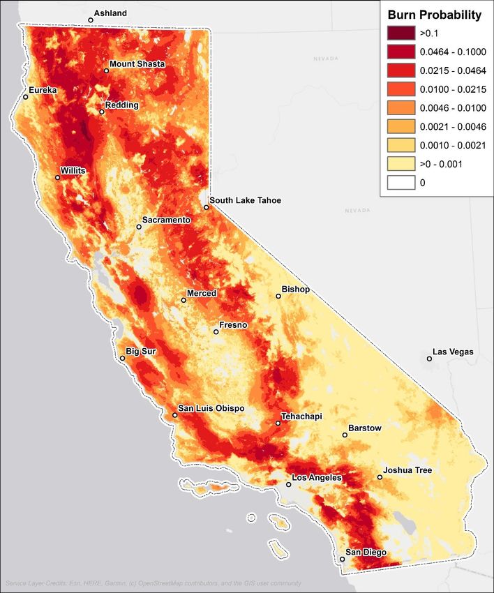
fire occurrence information to make a spatially resolved estimate of the contemporary likelihood
and intensity of wildfire across the landscape (Finney et al., 2011).
Due to the highly varied nature of weather and fire occurrence across the large landscape, we ran
FSim for each of the fourteen FOAs independently and then compiled the fourteen runs into a single
data product. For each FOA, we parameterized and calibrated FSim based on the location of
historical fire ignitions within the FOA, which is consistent with how the historical record is
compiled. We then used FSim to start fires only within each FOA but allowed those fires to spread
outside of the FOA. This, too, is consistent with how the historical record is compiled.

 MODEL CALIBRATION
FSim simulations for each FOA were calibrated to a 2020 trend analysis of historical large fire
occurrence including mean historical large-fire size, and mean annual area burned per million acres.
Calibration targets were adjusted upward from the mean values over the historical record based on
methods outlined in section 2.3.2.2. Additionally, care was taken to match simulated wildfire size
distributions to the historical record and allow for the occurrence of simulated fires larger than any
observed historically. While only large-fire sizes (>247.1 acres) were considered in calibration,
numerous small fires were also simulated. However, the impact of small fires on landscape-level
burn probability is negligible.
To calibrate each FOA, we started with baseline inputs and a starting rate-of-spread adjustment
(ADJ) factor file informed by experience on previous projects. All runs were completed at 120-m
resolution. Each FOA was calibrated separately, and final simulations were run with 10,000
iterations. The fourteen FOAs were then integrated into an overall result for the analysis area.

 INTEGRATING FOAS
We used the natural-weighting method of integrating adjacent FOAs that we developed on an
earlier project (Thompson et al., 2013b). With this method, well within the boundary of a FOA
(roughly 30 km from any boundary), the results are influenced only by that FOA. Near the border
with another FOA, the results will be influenced by that adjacent FOA. The weighting of each FOA
is in proportion to its contribution to the overall burn probability at each pixel.

2.5 WILDFIRE MODELING RESULTS
The FSim model produces estimates of burn probability as well as measures of fire intensity
including flame length exceedance probability, conditional flame length, and mean fireline intensity.
While FSim does generate measures of wildfire intensity, the WildEST derived intensity estimates
(described below in section 3) are more reliable than those generated stochastically within FSim.
The WildEST intensity values were used in all developed effects analyses. FSim generated 120-m
resolution estimates of burn probability. These results were further downscaled to 30-m resolution
using a methodology described in section 2.5.1 and presented in Figure 12.

 20

UPSAMPLING FSIM RESULTS
FSim’s stochastic simulation approach can be computationally intensive and therefore, time
constraining on large landscapes. A challenge, therefore, is to determine a resolution sufficiently
fine to retain detail in fuel and terrain features yet produce calibrated results in a reasonable
timeframe. Moreover, HVRA are often mapped at the same resolution as the final BP produced by
FSim. To enable greater resolution on HVRA mapping, we chose to upsample the FSim burn
probability (BP) rasters to 30 m.
The FSim fire modeling included custom burnable-urban fuel models. Without accounting for any
potential burnability in developed areas, simulated wildfires would stop at the edge of burnable
fuel. To address this issue, we allow fires to spread through burnable-urban pixels, which produces
simulated fire perimeters that can continue spreading through developed areas. However, because
of the many unknowns and challenges in modeling the potential for home-to-home spread in
landscape-scale fire modeling, we ultimately minimize the influence of burn probability values
associated with burnable-urban pixels and instead prefer to smooth probabilities from adjacent
wildlands within a specified distance as described below.
We upsampled the FSim BP raster using a multi-step process. First, we used the ESRI ArcGIS Focal
Statistics tool to perform two rectangular, low-pass filters at the 120-m resolution, calculating the
mean value of burnable pixels only (including burn probability values on burnable-urban pixels),
within a 3-pixel by 3-pixel moving window. These steps allowed us to “backfill” burnable pixels at 30
m that were coincident with non-burnable fuel at 120 m. We subsequently resampled the 120-m
FSim BP raster to 30 m using bilinear resampling. If, after running two low-pass filters, burnable
pixels had BP values of zero, we set a threshold value of 1-in-10,000 (0.001, the lowest BP value
resulting from our FSim simulations) to avoid assigning zero probability values on burnable pixels
with some burning potential.
We then smoothed burn probability values from nearby burnable fuel onto adjacent non-burnable
pixels to capture the low likelihood, but high consequence event of an urban conflagration. Before
running the smoothing steps, we masked the 30-m resampled raster to burnable pixels only,
removing BP values from burnable-urban pixels. Additionally, we removed BP values from small,
burnable islands less than 500 ha. The purpose of removing burnable urban, non-burnable fuel, and
small burnable islands is to prevent smoothing from these pixels, and in particular, to prevent golf
courses and urban parks from spreading wildfires to nearby homes.
The resulting resampled raster was then smoothed again using the ESRI ArcGIS Focal Statistics tool
to perform three low-pass filters at a 300 m resolution, allowing for spread from burnable pixels to
nearby non-burnable pixels. Each focal smoothing operation incrementally reduces burn
probability by including zero values on non-burnable pixels (other than water and ice) in the focal
mean calculation. This reduces burn probability on non-burnable fuel relative to the burnable fuel
nearby. The 900 m smoothing distance is consistent with work by Caggiano et al. (2020) showing
that all home losses to wildfire from 2000 to 2018 were within 850 m of wildland vegetation. By
removing the modeled BP on burnable-urban pixels, and in its place smoothing burn probability
onto those pixels, we reduce wildfire likelihood and control the distance those values are spread. If
small burnable islands were not populated through BP smoothing, they were assigned a threshold
value of 1-in-100,000 (0.00001).

 21

Figure 12. Map of integrated FSim burn probability results for the California study area at 30-m resolution.

 22

3 Wildfire Behavior Characteristics

 3.1 OVERVIEW OF METHODS
 To estimate wildfire characteristics across California we used a scripted geospatial modeling
 process called WildEST (for Wildfire Exposure Simulation Tool). WildEST uses the command-line
 version of FlamMap to perform 216 basic deterministic simulations of fire behavior characteristics
 for a range of weather types (combinations of wind speed, wind direction, fuel moisture content).
 Additionally, we integrate the dead fuel moisture conditioning feature of FlamMap, so dead fuel
 moisture content is sensitive to canopy cover and topography (slope, aspect, and elevation). We
 also use pre-calculated Wind Ninja grids representing terrain-adapted wind speed and direction.
 These grids were generated at 120-m resolution then upsampled to 30-m resolution before use in
 FlamMap.
 Rather than weighting the 216 results solely according to the temporal relative frequencies (TRFs)
 of the weather types, the WildEST process integrates results by weighting them according to their
 weather type probabilities (WTP), which gives higher weight to high-spread conditions into the
 calculations. The process of developing the WTP rasters is described in Section 3.1.2 below.
 The majority of WildEST results apply to the head of the fire. However, for use in fire-effects
 calculations, WildEST also generates Flame-Length Probability rasters (FLPs) that incorporate non-
 heading spread directions (Scott 2020), for which fire intensity is considerably lower than at the
 head of the fire. These "fire-effects FLPs" or “NVC FLPs" are analogous to FLP rasters produced by
 FSim.
 We use this weather type probability (WTP) weighting process in WildEST to produce headfire
 characteristics rasters (e.g., mean flame length), fire-type probability rasters, ember characteristics
 rasters, and non-heading characteristics rasters (for use in an effects analysis). Together, these
 rasters are useful for mapping the fire behavior that characterizes each pixel on the landscape. Each
 output is described in the respective following sections 3.2.1 - 3.3.2.

 FSIM VERSUS WILDEST
 Our use of command-line FlamMap in WildEST for this landscape-scale hazard assessment is a
 departure from what has been standard practice for USFS wildfire risk assessments that use FSim.
 Typically, such hazard assessments have used FSim for both the wildfire likelihood (burn
 probability) and wildfire intensity (flame-length probability) components of the assessment.
 Pyrologix developed the WildEST process to address a few shortcomings present when using FSim
 for fire intensity results.

 SP ATIAL RESOLUTION
 The spatial resolution (grid cell size) is limited to the resolution run for the main FSim fire
 occurrence modeling. For national-scale projects the resolution is 270 m; for CAL the resolution
 was 120 m. Even though fuelscape information is available from LANDFIRE at 30-m resolution,

 23

FSim cannot use that resolution due to excessive run time. In contrast, WildEST can run on large
landscapes at 30-m resolution.

 MODEL TYP E
FSim is a Monte Carlo simulator, so the fire intensity results it can produce are limited to 1) the
mean fireline intensity of simulated fires that burned each grid cell, and 2) the conditional
probability that flame length will be in each of six flame-length classes, called Fire Intensity Levels
(FILs). In FSim, flame length always accounts for the effect of relative spread direction (heading,
flanking, backing). Because the flame-length probabilities (FLPs) are determined by tallying the
relative fraction of times a grid cell burned in each FIL, they suffer from a problem of low sample
size, especially in places where BP is low. For example, where BP is 1-in-500 (0.002), a pixel would
burn 20 times over 10,000 iterations. The flame length of those 20 fires is tallied into six flame-
length bins. That is a small sample size to provide a stable estimate of the true flame-length
probabilities. Running FSim a second time could generate different FLPs for the same pixel.
WildEST is deterministic, so it does not suffer from a Monte Carlo simulator's sample-size problem.
And WildEST can be used to generate both headfire and non-heading fire intensity results.

 FIRE CHARACTERISTICS PRODUCED
FSim produces only two measures of fire intensity for each simulation: mean fireline intensity (MFI)
and flame-length probability (FLP) for six Fire Intensity Levels.
In contrast, we use WildEST to generate a wide array of fire characteristics, including the rate of
spread, heat per unit area, type of fire, crown fraction burned, and maximum ember travel distance.
These additional fire characteristics allow the calculation of additional measures of wildfire hazard,
including ember production and ember load, and Suppression Difficulty Index.

 SP ATIAL PRECISION OF WEATHER DATA
FSim is limited to using just one stream of weather for a large area (millions of acres). FSim does not
support dead fuel moisture conditioning, which accounts for the effects of elevation, canopy cover,
slope steepness, and aspect on dead fuel moisture content. FSim has limited support for applying
terrain-adapted winds using WindNinja.
WildEST uses gridded historical weather data at a spatial resolution of 2 km for CAL (coarser for
areas outside of California). We use both fuel moisture conditioning and WindNinja at 30-m
resolution to produce continuously variable fire characteristics results free of seamlines due to
weather inputs.

 TOP OLOGY EFF ECTS
One advantage of FSim is that it inherently accounts for any effects of fire spread topology4 on fire
intensity. For example, the land on the lee side of a large nonburnable feature (such as a lake, for

4
 Fire spread topology is the network of possible fire spread pathways given the fire environment.

 24

example) is less likely than other land to experience a headfire, because a headfire cannot spread
across the lake; instead, a fire must flank past this location, resulting in lower fire intensity. This
topology effect is pronounced for short-duration fires or when there is a single fire-carrying wind
direction. If fire can be carried across the landscape in multiple directions, the topology effect is
smaller.
WildEST cannot address such topological effects. Each location is evaluated using only the fuel,
weather, and topography at the location, with no consideration for adjacent nonburnable features
that could potentially reduce intensity by reducing the potential for heading spread.

 WEATHER TYPE PROBABILITY RASTERS
We used a bias-corrected, 2-km gridded, hourly weather data produced by the Desert Research
Institute using the Weather Research and Forecasting (WRF) weather model (version 3.5.1;
Skamarock et al. 2008), covering the period 2003-2018, to generate 30-m resolution Weather-
Type Probability (WTP) rasters seamlessly covering the state. For each hour in the 2003-2018
timeframe, we first calculated an area burned index (ABI) as follows:
 = ∗ 2 ∗ 
where SPI is the Schroeder Probability of Ignition (Schroeder 1969), a function of temperature and
fine fuel moisture content, WS is the open wind speed in MPH, and burn minutes is defined from a
lookup table (Table 4) as a function of wind speed and daily Energy Release Component percentiles.

Table 4. Burn minutes table for calculating area burned index (ABI).

 Wind Speed Bin ERC < 80th ERC 80-90th ERC 90-97th ERC >= 97th
 (MPH) percentile percentile percentile percentile
 0-3 30 30 30 30

 3-8 30 30 60 120

 8-13 30 60 120 180
 13-18 60 120 180 240

 18-23 120 180 240 300

 23-28 180 240 300 450
 28-33 240 300 450 600

 33-38 300 450 600 600

 >= 38 450 600 600 600

 25

The hourly ABI values were then summed across the timeframe within specific weather scenarios,
which are defined by wind speed, wind direction, and moisture condition bins.
There are nine wind speed bins:
 0-3, 3-8, 8-13, 13-18, 18-23, 23-28, 28-33, 33-38, and >= 38 MPH

There are eight wind direction bins:
 337.5-22.5, 22.5-67.5, 67.5-112.5, 112.5-157.5, 157.5-202.5, 202.5-247.5, 247.5-292.5, 292.5-337.50

And there are three 1-hr timelag moisture content bins:

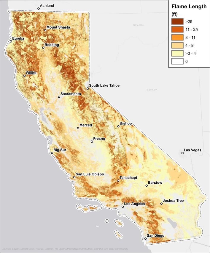
FLAME LENGTH (FL)
Flame length is the weighted-average flame length in feet for a given pixel in the fuelscape, including
any contribution of crown fire under a given weather type (Figure 15). Weighted FL is calculated as
the sum-product of 216 FL rasters and their corresponding WTPs.

 FIRE-TYPE PROBABILITY (FTP)
Fire-type probability rasters indicate the conditional probability that a given pixel will experience a
certain type of fire. At a given pixel, the sum of fire-type probabilities equals 1 (100%). The FTPs
indicate the range of fire types that can be produced by the fire environment and their relative
prevalence.
We define seven fire types (Table 5):
 1. Non-fuel
 2. Surface fire
 3. Underburn5
 4. Low-grade passive crown fire
 5. Mid-grade passive crown fire
 6. High-grade passive crown fire
 7. Active crown fire

The non-fuel “fire type” is assigned to pixels that do not have burnable fuel in the fuelscape and
therefore do not experience any type of fire. The possible raster values for non-fuel probability are
either 0 (burnable fuel is present) or 1 (the pixel is nonburnable).
Similarly, the surface fire type is assigned to pixels with burnable fuel but without forest canopy
present. In these cases, surface fire is the only possibility. We distinguish this type from an
underburn because the latter indicates that crowning was possible, but not achieved. The raster
value for this fire-type probability is 1 if the pixel is burnable but does not have a canopy or 0 for all
other cases.
The remaining five fire types require a pixel to have 1) a burnable surface fuel model and 2) a tree
canopy present, representing the possibility of a crown fire under some conditions. Raster
probability values range from 0 to 1. Crown fire types are commonly classified as either passive or
active. But passive crown fire represents a large range of crowning behavior from a single tree
torching up to nearly continuous large-group torching. We, therefore, divided passive crown fire
into three sub-classes based on the crown fraction burned (CFB) estimated for the fire
environment. Crown fraction burned represents the fraction of the canopy fuel contributing to
overall rate of spread and intensity.

5
 The term underburn is used rather than surface fire to distinguish from the situation where there is no forest
canopy present.

 27

Table 5. The WildEST Type of Fire classification.

 Burnable land Forest canopy Crown Fraction
 Type of fire
 cover? present? Burned (%)
 Non-fuel No
 Surface Yes No

 Underburn Yes Yes 0

 Low-grade passive Yes Yes 0

“FIRE-EFFECTS” FLAME-LENGTH PROBABILITIES
All the WildEST results described thus far above apply to the head of a fire, but a free-burning
wildfire spreads in all directions and therefore exhibits a range of flanking and backing behavior in
addition to heading behavior. Flanking and backing fires exhibit a lower spread rate and intensity
than at the head of a fire (Catchpole et al., 1982; Catchpole et al., 1992) FSim and other stochastic
wildfire simulators inherently capture non-heading fire spread and intensity. The deterministic
approach we use in WildEST inherently captures only headfire spread and intensity, so we apply
adjustments to headfire intensity based on the geometry of an assumed fire spread ellipse (Scott
2020).
The FLP differences between heading and non-heading FLPs are illustrated in Figure 13, which is
an example fuel complex consisting of surface fire behavior fuel model TU5, with a canopy base
height of 0.3 m and a canopy bulk density of 0.11 kg/m3. For that fuel complex (and for the
climatology of that location), we estimate that headfire flame length will exceed 12 feet 66% of the
time the pixel burns, and never produce flame lengths less than 4 feet. After accounting for flanking
and backing behavior, we estimate flame length will exceed 12 feet only 42% of the time and will be
lower than four feet 5% of the time.
The WildEST non-heading characteristics include non-heading flame-length probabilities, which we
call “fire-effects” FLPs because they are designed for use in an Effects Analysis in a landscape
wildfire risk assessment as described in USFS GTR-315 (Scott and others 2013). These fire-effects
FLPs are a close analog to FSim’s FLPs and are used for the same purpose.
Like the headfire FLPs described above, we produce non-heading FLPs for the same six standard
flame-length classes (also called Fire Intensity Levels). Fire-effects flame-length probabilities are
shown in Figure 19.

 29

Figure 13. Headfire flame-length probabilities (top) and non-heading (or “fire effects”) flame-length probabilities (bottom).

 30

Figure 14. Map of WildEST 30-m Rate of Spread (m/min) for the CAL analysis area.

 31

Figure 15. Map of WildEST 30-m Mean Flame Length (ft) for the CAL analysis area.

 32