Copernicus Atmosphere Monitoring Service TEMPOral profiles (CAMS-TEMPO): global and European emission temporal profile maps for atmospheric ...
←
→
Page content transcription
If your browser does not render page correctly, please read the page content below

Earth Syst. Sci. Data, 13, 367–404, 2021
https://doi.org/10.5194/essd-13-367-2021
© Author(s) 2021. This work is distributed under
the Creative Commons Attribution 4.0 License.

        Copernicus Atmosphere Monitoring Service TEMPOral
        profiles (CAMS-TEMPO): global and European emission
                  temporal profile maps for atmospheric
                          chemistry modelling
              Marc Guevara1 , Oriol Jorba1 , Carles Tena1 , Hugo Denier van der Gon2 , Jeroen Kuenen2 ,
              Nellie Elguindi3 , Sabine Darras4 , Claire Granier3,5,6 , and Carlos Pérez García-Pando1,7
                                1 BarcelonaSupercomputing Center, 08034 Barcelona, Spain
                       2 Department of Climate, Air and Sustainability, TNO, Utrecht, the Netherlands
                     3 Laboratoire d’Aérologie, Université de Toulouse, CNRS, UPS, Toulouse, France
                                      4 Observatoire Midi-Pyrénées, Toulouse, France
                             5 NOAA Chemical Sciences Laboratory, Boulder, Colorado, USA
                            6 CIRES, University of Colorado Boulder, Boulder, Colorado, USA
                 7 ICREA, Catalan Institution for Research and Advanced Studies, 08010 Barcelona, Spain

                                  Correspondence: Marc Guevara (marc.guevara@bsc.es)

                                    Received: 1 July 2020 – Discussion started: 4 August 2020
                     Revised: 20 December 2020 – Accepted: 26 December 2020 – Published: 12 February 2021

      Abstract. We present the Copernicus Atmosphere Monitoring Service TEMPOral profiles (CAMS-TEMPO),
      a dataset of global and European emission temporal profiles that provides gridded monthly, daily, weekly and
      hourly weight factors for atmospheric chemistry modelling. CAMS-TEMPO includes temporal profiles for the
      priority air pollutants (NOx ; SOx ; NMVOC, non-methane volatile organic compound; NH3 ; CO; PM10 ; and
      PM2.5 ) and the greenhouse gases (CO2 and CH4 ) for each of the following anthropogenic source categories:
      energy industry (power plants), residential combustion, manufacturing industry, transport (road traffic and air
      traffic in airports) and agricultural activities (fertilizer use and livestock). The profiles are computed on a global
      0.1 × 0.1◦ and regional European 0.1 × 0.05◦ grid following the domain and sector classification descriptions of
      the global and regional emission inventories developed under the CAMS programme. The profiles account for
      the variability of the main emission drivers of each sector. Statistical information linked to emission variability
      (e.g. electricity production and traffic counts) at national and local levels were collected and combined with
      existing meteorology-dependent parametrizations to account for the influences of sociodemographic factors and
      climatological conditions. Depending on the sector and the temporal resolution (i.e. monthly, weekly, daily and
      hourly) the resulting profiles are pollutant-dependent, year-dependent (i.e. time series from 2010 to 2017) and/or
      spatially dependent (i.e. the temporal weights vary per country or region). We provide a complete description of
      the data and methods used to build the CAMS-TEMPO profiles, and whenever possible, we evaluate the repre-
      sentativeness of the proxies used to compute the temporal weights against existing observational data. We find
      important discrepancies when comparing the obtained temporal weights with other currently used datasets. The
      CAMS-TEMPO data product including the global (CAMS-GLOB-TEMPOv2.1, https://doi.org/10.24380/ks45-
      9147, Guevara et al., 2020a) and regional European (CAMS-REG-TEMPOv2.1, https://doi.org/10.24380/1cx4-
      zy68, Guevara et al., 2020b) temporal profiles are distributed from the Emissions of atmospheric Compounds
      and Compilation of Ancillary Data (ECCAD) system (https://eccad.aeris-data.fr/, last access: February 2021).

Published by Copernicus Publications.
368                                                                                          M. Guevara et al.: CAMS-TEMPO

1   Introduction                                                   European Emission Data for Episodes (GENEMIS) project
                                                                   are still considered as the main reference (Ebel et al., 1997;
Spatially and temporally resolved atmospheric emission in-         Friedrich and Reis, 2004). The original GENEMIS profiles
ventories are key to investigate and predict the transport and     were later used as a basis to derive two independent datasets:
chemical transformation of pollutants, as well as to develop       (i) the EMEP temporal profiles, which provide monthly,
effective mitigation strategies (e.g. Pouliot et al., 2015; Gal-   weekly and hourly weight factors that vary per emission
marini et al., 2017). During the last decade, global and re-       sector, country and pollutant (Simpson et al., 2012), and
gional inventories have substantially increased spatial resolu-    (ii) the Netherlands Organisation for Applied Scientific Re-
tion from ∼ 50 × 50 km (e.g. MACCity; Granier et al., 2011;        search (TNO) temporal profiles, which provide monthly,
EMEP-50 km; Mareckova et al., 2013) to ∼ 10 × 10 km or             weekly and hourly weight factors that vary per emission sec-
less (e.g. EMEP-0.1deg, Mareckova et al., 2017; TNO-               tor (Denier van der Gon et al., 2011). These two sets of pro-
MACC; Kuenen et al., 2014). Several datasets even pro-             files have become over time the reference datasets under the
vide emission maps for selected pollutants or study re-            framework of several European air quality modelling activ-
gions with resolutions as fine as 1 × 1 km (e.g. ODIAC2016,        ities, including the earlier Monitoring Atmospheric Compo-
Open-source Data Inventory for Anthropogenic CO2 , ver-            sition and Climate (MACC) project and the current Coperni-
sion 2016, Oda et al., 2018; Hestia-LA, Hestia fossil fuel         cus Atmosphere Monitoring Service (CAMS), among others.
CO2 emissions data product for the Los Angeles megacity;           Other widely used regional temporal profile datasets include
Gurney et al., 2019; Super et al., 2020). This improvement         the North American profiles provided by the Environmen-
is largely due to the emergence of new detailed, satellite-        tal Protection Agency (EPA) Clearinghouse for Inventories
based and open-access spatial proxies such as the population       and Emissions Factors (CHIEF) (US EPA, 2019a) and the
maps at 1 × 1 km proposed by the Global Human Settlement           monthly profiles provided by the Multi-resolution Emission
Layer (GHSL) project (Florczyk et al., 2019), the global           Inventory for China (MEIC; Li et al., 2017).
land cover maps at 300 × 300 m provided by the European               Our goal is to provide a new set of global and European
Space Agency Climate Change Initiative (ESA CCI, https:            temporal profiles. Current datasets typically use the same
//www.esa-landcover-cci.org/, last access: February 2021)          temporal profiles for certain sectors and/or regions. For ex-
or the georeferenced road traffic network distributed by           ample, ECLIPSE and EMEP share the same monthly profiles
OpenStreetMap (OSM, http://www.openstreetmap.org, last             for the energy sector in Europe and Russia. Similarly, TNO
access: February 2021). While a clear evolution is observed        and EDGAR share the same monthly profiles for residential
in terms of spatial resolution, the improvement of the tempo-      combustion and road transport (Friedrich and Reis, 2004),
ral representation in current state-of-the-art emission datasets   as well as for the energy industry (Veldt, 1992) and agricul-
has not been addressed much (Reis et al., 2011).                   ture (Asman, 1992). In these two datasets, temporal profiles
   Using global and regional emission inventories in atmo-         are mostly assumed to be both country- and meteorology-
spheric chemistry models requires the original aggregated          independent. The only exceptions are, in the case of EDGAR,
annual emissions to be broken down into fine temporal reso-        for the residential and agricultural sectors, which are approx-
lutions (ideally hourly) using emission temporal profiles (e.g.    imated as a function of the geographical zone: the seasonality
Borge et al., 2008; Bieser et al., 2011; Mues et al., 2014).       assumed in the Northern Hemisphere is shifted by 6 months
In practice, temporal profiles are normalized weight factors       in the Southern Hemisphere, and a flat profile is assumed
for each hour of the day, day of the week and month of the         along the Equator. In the case of EMEP, the reported monthly
year. At the global scale, the most commonly used emission         and weekly profiles do consider differences across countries
temporal profiles are the monthly factors provided by the air      but are primarily based on old sources of information from
pollutant and greenhouse gas Emission Database for Global          the 1990s and beginning of the 2000s and subsequently ne-
Atmospheric Research inventory (EDGARv4.3.2; Janssens-             glect behavioural changes that may have happened over the
Maenhout et al., 2019) and the Evaluating the Climate and          last years. Similarly, road transport weekly and hourly fac-
Air Quality Impacts of Short-Lived Pollutants inventory            tors reported by TNO are based on long time series of Dutch
(ECLIPSEv5.a; Klimont et al., 2017). Also at the global            data registering the traffic intensity between 1985 and 1998.
level, the Temporal Improvements for Modeling Emissions            Moreover, variable climate conditions and changes in meteo-
by Scaling (TIMES) dataset was produced to represent the           rology that may cause differences in the temporal weight fac-
weekly and hourly variability for global CO2 emission in-          tors within a country are not accounted for. In order to over-
ventories (Nassar et al., 2013). More recently, Crippa et          come this limitation, the ECLIPSE monthly profiles for the
al. (2020) developed a new set of high-resolution temporal         residential combustion sector were computed using global
profiles for the EDGAR inventory which allows for produc-          gridded temperature data and provided as monthly shares for
ing monthly and hourly emission time series and grid maps.         each grid cell (Klimont et al., 2017).
   At the European level, the temporal factors provided by            This work presents the Copernicus Atmosphere Monitor-
the University of Stuttgart (Institute of Energy Economics         ing Service TEMPOral profiles (CAMS-TEMPO), a new
and Rational Energy Use, IER) as part of the Generation of         dataset of global and European emission temporal profiles

Earth Syst. Sci. Data, 13, 367–404, 2021                                            https://doi.org/10.5194/essd-13-367-2021
M. Guevara et al.: CAMS-TEMPO                                                                                                  369

for atmospheric chemistry modelling. The development of           based on Huang et al. (2017). A comparison of CAMS-
CAMPS-TEMPO comes from the need to overcome the                   GLOB-ANT emissions to the other inventories is presented
aforementioned limitations of current profiles (i.e. use of an    in Elguindi et al. (2020b).
outdated source of information and neglection of the tem-            The CAMS regional emissions are being prepared for air
poral variation of emissions across species and countries         pollutants and greenhouse gases (CAMS-REG_AP/GHG), in
or regions) and to improve the representation of the emis-        support of the CAMS regional production systems and policy
sion temporal variations, which was defined as a priority         tools. The inventory is built up largely using the official re-
task within the Copernicus global and regional emissions          ported emission data from individual countries in Europe for
service (CAMS_81) directly supporting the CAMS produc-            each source category, which has the main advantage that it
tion chains (https://atmosphere.copernicus.eu/, last access:      takes into account country-specific information on technolo-
February 2021). Multiple socio-economic, statistical and me-      gies, practices and associated emissions. Where these data
teorological data were collected and processed to create          were either unavailable or not fit for purpose, these were re-
the profiles. The CAMS-TEMPO dataset includes monthly,            placed with other estimates. Then, a consistent spatial distri-
weekly, daily and hourly temporal profiles for the priority       bution is applied across Europe at a resolution of 0.1 × 0.05◦
air pollutants (NOx ; SOx ; NMVOC, non-methane volatile           by means of using proxies for each source category of emis-
organic compound; NH3 ; CO; PM10 ; and PM2.5 ) and the            sions. These proxies include among others point source emis-
greenhouse gases (CO2 and CH4 ) and each of the follow-           sions from E-PRTR (European Pollutant Release and Trans-
ing anthropogenic source categories: energy industry, resi-       fer Register), road networks, land use and population density
dential combustion, manufacturing industry, transport (road       information. Shipping emissions are taken from the STEAM
traffic and air traffic in airports) and agriculture. Depending   (Ship Traffic Emission Assessment Model) model (Johans-
on the sector and temporal resolution, the profiles are either    son et al., 2017). By also providing speciation profiles for PM
fixed (spatially constant) or vary spatially by country or re-    (particulate matter) and VOCs (volatile organic compounds),
gion and can be pollutant-dependent and/or year-dependent.        as well as default height profiles, the dataset is fit for purpose
The CAMS-TEMPO profiles introduce multiple novel as-              for air quality modelling at the European scale. Different ver-
pects when compared to the current profiles used for air qual-    sions of the CAMS regional emissions are available, with the
ity modelling, including (i) pollutant dependency, (ii) spatial   latest version (v4.2) covering the years 2000–2017 having
variability and (iii) meteorological influence. Table 1 sum-      been produced in early 2020. The methodology used for an
marizes and compares the main characteristics of the CAMS-        earlier version of this inventory is available (Kuenen et al.,
TEMPO profiles with the ones reported in other datasets           2014), and a new publication is currently in preparation for
including TNO (Denier van det Gon et al., 2011), EMEP             the latest version (Kuenen et al., 2021).
(Simpson et al., 2012), EDGARv4.3.2 (Janssens-Maenhout               The paper is organized as follows. Section 2 describes,
et al., 2019) and EDGARv5 (Crippa et al., 2020) regarding         for each sector, the approaches and sources of information
spatial coverage, temporal and spatial resolution, and year or    used to develop the CAMS-TEMPO profiles. Section 3 dis-
meteorology dependency.                                           cusses the obtained temporal profiles and compares them to
   The CAMS-TEMPO profiles were created following the             currently available datasets. Section 4 provides a description
domain descriptions (resolution and geographical area cov-        of the data availability, and finally Sect. 5 presents the main
ered) and emission sector classification system defined in        conclusions of this work.
the CAMS global anthropogenic inventory (CAMS-GLOB-
ANT) and CAMS regional inventory for air pollutants and
                                                                  2     Methodology
greenhouse gases (CAMS-REG_AP/GHG), also developed
under CAMS_81 (Granier et al., 2019).                             2.1    Overview
   The CAMS-GLOB-ANT dataset (Elguindi et al., 2020a)
is a global emission inventory developed for the years 2000–      The following subsections describe the input data and
2020 at a spatial resolution of 0.1 × 0.1◦ in support of          methodologies used to compute the CAMS-TEMPO emis-
the CAMS global simulations. The data are based on the            sion temporal profiles for each targeted sector: (i) energy in-
EDGARv4.3.2 annual emissions developed by the European            dustry (Sect. 2.2), (ii) residential and commercial combustion
Commission Joint Research Centre (JRC, Crippa et al., 2018)       (Sect. 2.3), (iii) manufacturing industry (Sect. 2.4), (iv) road
for the years 2000–2012. After 2012, the emissions are ex-        transport (Sect. 2.5), (v) aviation (Sect. 2.6), and (vi) agricul-
trapolated to the current year using linear trend fits to the     ture (Sect. 2.7).
years 2011–2014 from the CEDS (Community Emissions                   The CAMS-TEMPO dataset consists of a collection of
Data System) global inventory (Hoesly et al., 2018), which        global and regional temporal factors that follow the do-
provides historical emissions for the Sixth Assessment Re-        main description and sector classification reported by the
port (AR6) of the IPCC (Intergovernmental Panel on Climate        CAMS-GLOB-ANT and CAMS-REG_AP/GHG emission
Change). Emissions are provided for the main pollutants and       inventories. In order to better distinguish between the
greenhouse gases, together with a speciation of NMVOCs            two sets of profiles, we refer to them as CAMS-GLOB-

https://doi.org/10.5194/essd-13-367-2021                                            Earth Syst. Sci. Data, 13, 367–404, 2021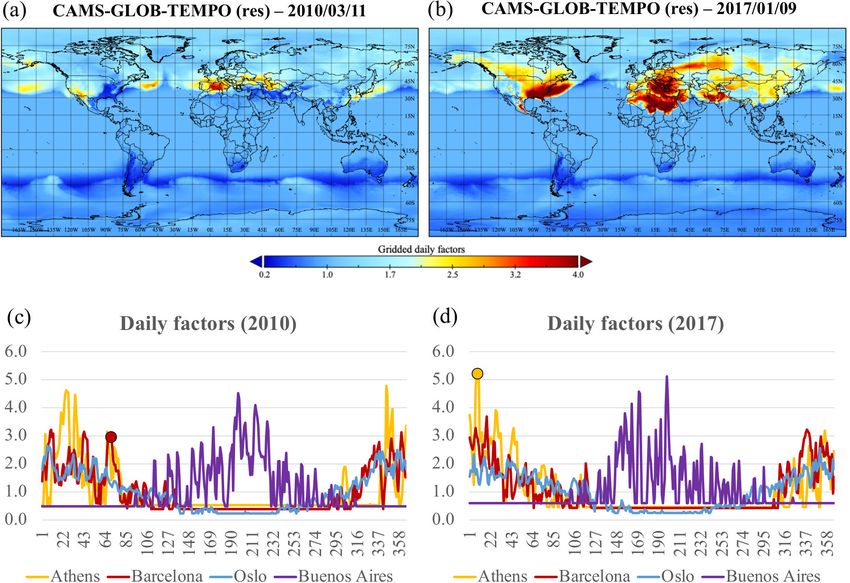
370                                                                                                                   M. Guevara et al.: CAMS-TEMPO

Table 1. Main characteristics of the temporal profiles developed in this work compared to those reported in other datasets including TNO
(Denier van det Gon et al., 2011), EMEP (Simpson et al., 2012), EDGARv4.3.2 (Janssens-Maenhout et al., 2019) and EDGARv5 (Crippa et
al., 2020) regarding spatial coverage, temporal and spatial resolution, and year or meteorology dependency.

  Sector            Dataset       Spatial coverage   Temporal resolution              Spatial resolution                          Year or meteorology dependency
  Energy industry   This work     Global, EU         Monthly, weekly, hourly          Country-dependent                           No
                    TNO           EU                 Monthly, weekly, hourly          Fixed                                       No
                    EMEP          EU                 Monthly, weekly, hourly          Country-dependent                           No
                    EDGARv4.3.2   Global             Monthly                          3 geo-regions                               No
                    EDGARv5       Global             Monthly, weekly, hourly          Country-dependent                           Yes (monthly profiles)
  Residential       This work     Global, EU         Monthly, weekly, daily, hourly   Grid cell level (monthly, daily profiles)   Yes (monthly, daily profiles)
  combustion        TNO           EU                 Monthly, weekly, hourly          Fixed                                       No
                    EMEP          EU                 Monthly, weekly, hourly          Country-dependent                           No
                    EDGARv4.3.2   Global             Monthly                          3 geo-regions                               No
                    EDGARv5       Global             Monthly, weekly, hourly          Country-dependent                           Yes (monthly profiles)
  Manufacturing     This work     Global, EU         Monthly, weekly, hourly          Country-dependent (monthly profiles)        No
  industry          TNO           EU                 Monthly, weekly, hourly          Fixed                                       No
                    EMEP          EU                 Monthly, weekly, hourly          Country-dependent                           No
                    EDGARv4.3.2   Global             Monthly                          Fixed                                       No
                    EDGARv5       Global             Monthly, weekly, hourly          23 world regions                            No
  Road              This work     Global, EU         Monthly, weekly, hourly          Grid cell level                             Yes (EU monthly profiles)
  transport         TNO           EU                 Monthly, weekly, hourly          Fixed                                       No
                    EMEP          EU                 Monthly, weekly, hourly          Country-dependent                           No
                    EDGARv4.3.2   Global             Monthly                          Fixed                                       No
                    EDGARv5       Global             Monthly, weekly, hourly          23 world regions                            No
  Aviation          This work     EU                 Monthly, weekly, hourly          Country-dependent (monthly profiles)        No
                    TNO           EU                 Monthly, weekly, hourly          Fixed                                       No
                    EMEP          EU                 Monthly, weekly, hourly          Country-dependent                           No
                    EDGARv4.3.2   Global             Monthly                          Fixed                                       No
                    EDGARv5       Global             Monthly, weekly, hourly          Fixed                                       No
  Agriculture       This work     Global, EU         Monthly, weekly, daily, hourly   Grid cell level (monthly, daily profiles)   Yes (monthly, daily profiles)
  (livestock)       TNO           EU                 Monthly, weekly, hourly          Fixed                                       No
                    EMEP          EU                 Monthly, weekly, hourly          Country-dependent                           No
                    EDGARv4.3.2   Global             Monthly                          3 geo-regions                               No
                    EDGARv5       Global             Monthly, weekly, hourly          Fixed                                       No
  Agriculture       This work     Global, EU         Monthly, weekly, daily, hourly   Grid cell level (monthly, daily profiles)   Yes (monthly, daily profiles)
  (fertilizers)     TNO           EU                 Monthly, weekly, hourly          Fixed                                       No
                    EMEP          EU                 Monthly, weekly, hourly          Country-dependent                           No
                    EDGARv4.3.2   Global             Monthly                          3 geo-regions                               No
                    EDGARv5       Global             Monthly, weekly, hourly          Fixed                                       No
  Agriculture       This work     Global, EU         Monthly, weekly, hourly          Grid cell level (monthly profiles)          No
  (agricultural-    TNO           EU                 Monthly, weekly, hourly          Fixed                                       No
  waste burning)    EMEP          EU                 Monthly, weekly, hourly          Country-dependent                           No
                    EDGARv4.3.2   Global             Monthly                          3 geo-regions                               No
                    EDGARv5       Global             Monthly, weekly, hourly          23 world regions                            No

TEMPO (https://doi.org/10.24380/ks45-9147, Guevara et                             TEMPO and 0.1 × 0.05◦ for CAMS-REG-TEMPO. In the
al., 2020a, global temporal profiles associated with the                          case of CAMS-REG-TEMPO, the domain covered by the
CAMS-GLOB-ANT inventory) and CAMS-REG-TEMPO                                       dataset is 30◦ W–60◦ E and 30–72◦ N.
(https://doi.org/10.24380/1cx4-zy68, Guevara et al., 2020b,                          Tables 2 and 3 summarize the characteristics of each tem-
regional European temporal profiles associated with the                           poral profile included in the CAMS-GLOB-TEMPO and
CAMS-REG_AP/GHG inventory). Depending on the pollu-                               CAMS-REG-TEMPO datasets, respectively. The sector clas-
tant source and temporal resolution (i.e. monthly, weekly,                        sification for each case corresponds to those used in CAMS-
daily and hourly), the resulting profiles are reported as spa-                    GLOB-ANT and CAMS-REG_AP/GHG. The specificity of
tially invariant (i.e. a unique set of temporal weights for the                   the computed profiles depends upon the degree of sectoral
entire domain, Tables A1 to A4 in Appendix A of this work)                        disaggregation used in the original CAMS inventories. For
or gridded values (i.e. temporal weights vary per grid cell).                     example, the CAMS-GLOB-ANT dataset reports emissions
Similarly, depending on the characteristics of the input data                     from power and heat plants and refineries under the same
used and approaches to compute the profiles, these can be                         sector (“ene”, see Table 2), and therefore a common set of
year-dependent and/or pollutant-dependent. The spatial reso-                      temporal profiles had to be assumed for the two types of fa-
lution of the gridded profiles is 0.1 × 0.1◦ for CAMS-GLOB-                       cilities. In contrast, the CAMS-REG_AP/GHG inventory re-

Earth Syst. Sci. Data, 13, 367–404, 2021                                                                   https://doi.org/10.5194/essd-13-367-2021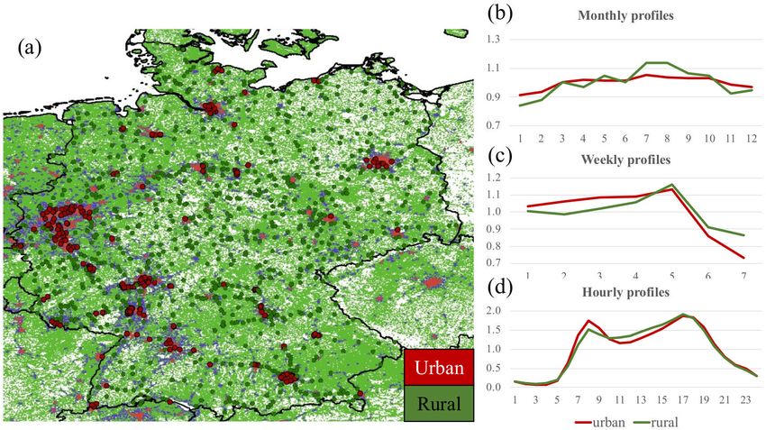
M. Guevara et al.: CAMS-TEMPO                                                                                                  371

ports power and heat plants under the GNFR_A (Gridding                 continuous emission monitoring system (CEMS). The
Nomenclature for Reporting) category (public power) and                information collected includes hourly NOx , SOx and
refineries under sector GNFR_B (industry), together with               heat input data for individual power plants in the years
all manufacturing industries (Table 3). All the assumptions            2011 and 2014.
made regarding this topic are clearly stated in each subsec-
tion.                                                               – The IEA electricity statistics. The International Energy
   For both CAMS-GLOB-TEMPO and CAMS-                                 Agency (IEA; IEA, 2021) provides consistent electric-
REG_AP/GHG, the sum of all temporal weight factors                    ity statistics split by generation type (i.e. total fossil fu-
is equal to 12 for monthly profiles, 7 for weekly profiles, 365       els, nuclear, hydro, and geothermal or other) and coun-
or 366 (in the case of a leap year) for daily profiles, and 24        try. The information collected included monthly data for
for hourly profiles. Note that the hourly temporal profiles in        the years 2010 to 2017 for each member country of the
CAMS-TEMPO are provided in local standard time (LST).                 Organisation for Economic Co-operation and Develop-
The conversion from LST to coordinated universal time                 ment (OECD).
(UTC) as a function of time zones is a process that needs
                                                                    – The MBS Online. The Monthly Bulletin of Statistics
to be performed by the final user. Time zone adjustments is
                                                                      (MBS; MBS, 2018) is a database of the United Nations
a process typically performed by the emission processing
                                                                      with a focus on national economic and social statistics.
systems or tools designed to adapt emission data to the air
                                                                      It provides monthly data of the total electricity gross
quality modelling requirements (e.g. Guevara et al., 2019).
                                                                      production per country. The information collected in-
                                                                      cluded data for the year 2015.
2.2   Energy industry
                                                                     Figure 1a illustrates the spatial coverage of the com-
The temporal profiles computed for the energy industry are        piled dataset by source of information (i.e. ENTSO-E, US
reported under the ene sector in CAMS-GLOB-TEMPO and              EPA, IEA and MBS). Overall, main emission producers (e.g.
the GNFR_A category in CAMS-REG-TEMPO. The tempo-                 China, India, Europe and North America) are covered, while
ral variability of emissions from this sector was estimated       most of the countries with no information available are lo-
from electricity production statistics under the assumption       cated in South America and Africa. For those countries with
that it largely depends upon the combustion of fossil fuels       no data, the TNO profiles reported under the energy sector
in power and heat plants. This approximation is consistent        (Denier van der Gon et al., 2011) are used.
with the definition of the GNFR_A sector in the CAMS-                The compiled data were first analysed to assess whether
REG_AP/GHG dataset. The representativeness of the com-            interannual variability is important for this sector. Seasonal
puted profiles is likely lower in CAMS-GLOB_TEMPO be-             cycles were computed for different years (2010–2017) and
cause the ene sector also includes other facilities such as re-   countries using the IEA statistics. In the majority of the coun-
fineries.                                                         tries analysed, the monthly profiles were found to be con-
   As shown in Tables 2 and 3, the profiles reported for this     sistent through the different years and to present small in-
sector include pollutant- and country-dependent monthly,          terannual variations (Fig. S1 in the Supplement). Although
weekly and hourly factors. The electricity production dataset     some studies have pointed out a temperature dependence of
compiled to derive profiles for this sector were as follows:      the monthly electricity generation in power plants (Thiruchit-
  – The ENTSO-E Transparency Platform. The European               tampalam, 2014), we neglected it at present. Consequently,
    Network of Transmission System Operators for Elec-            we assume the monthly temporal profiles for this sector to be
    tricity (ENTSO-E; Hirth et al., 2018; ENTSO-E, 2018)          the average over all the available years of data.
    centralizes the collection and publication of the elec-
    tricity generation per production type for each Euro-         2.2.1   Monthly profiles
    pean member state. The information published by the
    Transparency Platform is collected from data providers        For European countries, monthly profiles were derived using
    such as transmission system operators (TSOs), power           the ENTSO-E dataset. The analysis of the data showed that
    exchanges or other qualified third parties. The informa-      the seasonality of electricity production varies significantly
    tion collected included production data (in MW) per           by fuel type (Fig. S1). The different use of energy sources
    country and fuel type (i.e. lignite, hard coal, natural       (i.e. lignite, hard coal, natural gas, biomass and oil) implies
    gas, oil and biomass) at monthly (years 2010–2014) and        that temporal patterns will also vary from one pollutant to
    hourly (years 2015–2017) levels.                              another. For each month, country and pollutant, profiles were
                                                                  calculated following Eq. (1):
  – The US EPA emission modelling platform. The Environ-
    mental Protection Agency (EPA; US EPA, 2019a) main-
                                                                             Xn                   FSc,f · EFf,p
                                                                  Mm,c,p =      f =1
                                                                                       Mm,c,f   n                      ,        (1)
    tains an emission modelling platform that includes pro-                                     P
                                                                                                       FSc,f · EFf,p
    cessed and clean hourly emission data derived from a                                        f =1

https://doi.org/10.5194/essd-13-367-2021                                               Earth Syst. Sci. Data, 13, 367–404, 2021
372                                                                                                                           M. Guevara et al.: CAMS-TEMPO

Table 2. Main characteristics of the CAMS global temporal profiles (CAMS-GLOB-TEMPO) reported by sector and temporal resolution
(monthly, daily, weekly and hourly). The text between brackets gives information on the spatial resolution and pollutant and year dependency
of each profile. Gridded indicates that the profile varies per grid cell within a country; per country indicates that the profile varies only per
country; fixed indicates that the profile is spatially invariant; year-independent indicates that the profiles does not vary per year; year-
dependent indicates that the profile varies per year; pollutant-independent indicates that the same profile is proposed for all pollutants (NOx ,
SOx , NMVOC, NH3 , CO, PM10 , PM2.5 , CO2 and CH4 ); pollutant-dependent indicates that the profile varies per pollutant; per day type
indicates that the profile varies as a function of the day (weekday, Saturday and Sunday). The symbol “–” denotes that no profile is proposed.

                                                                                            = 365 or 366)a
                                                    P                                   P                                P                              P
  Sector     Description                   Monthly ( = 12)                    Daily (                            Weekly ( = 7)               Hourly (       = 24)
  ene        Power generation              (Per country, year-                –                                  (Per country, year-         (Per country, year-
             (power and heat plants,       independent, pollutant-                                               independent, pollutant-     independent, pollutant-
             refineries, others)           dependent)                                                            dependent)                  dependent)
  ind        Industrial process            (Per country, year-                –                                  (Fixed, year-independent,   (Fixed, year-independent,
                                           independent, pollutant-                                               pollutant-independent)b     pollutant-independent)b
                                           independent)
  res        Other stationary              (Gridded, year-dependent,          (Gridded, year-dependent,          (Fixed, year-independent,   (Gridded, year-
             combustion                    pollutant-independent)             pollutant-independent)             pollutant-independent)b     independent, pollutant
                                                                                                                                             -dependent)
  fef        Fugitives                     (Fixed, year-independent,          –                                  (Fixed, year-independent,   (Fixed, year-independent,
                                           pollutant-independent)b                                               pollutant-independent)b     pollutant-independent)b
  slv        Solvents                      (Fixed, year-independent,          –                                  (Fixed, year-independent,   (Fixed, year-independent,
                                           pollutant-independent)b                                               pollutant-independent)b     pollutant-independent)b
  tro        Road transportation           (Gridded, year-                    –                                  (Gridded, year-             (Year-independent,
                                           independent, pollutant-                                               independent, pollutant-     pollutant-independent,
                                           independent)                                                          independent)                per day type)
  shp        Ships                         (Fixed, year-independent,          –                                  (Fixed, year-independent,   (Fixed, year-independent,
                                           pollutant-independent)b                                               pollutant-independent)b     pollutant-independent)b
  tnr        Off-road transportation       (Fixed, year-independent,          –                                  (Fixed, year-independent,   (Fixed, year-independent,
                                           pollutant-independent)b                                               pollutant-independent)b     pollutant-independent)b
  swd        Solid waste and waste         (Fixed, year-independent,          –                                  (Fixed, year-independent,   (Fixed, year-independent,
             water                         pollutant-independent)b                                               pollutant-independent)b     pollutant-independent)b
  mma        Agriculture (livestock)       NH3 and NOx                        NH3 and NOx                        (Fixed, year-independent,   (Fixed, year-independent,
                                           (gridded, year-dependent)          (gridded, year-dependent)          pollutant-independent)b     pollutant-independent)b
                                           Others
                                           (fixed, year-independent)
  agr        Agriculture (fertilizers      NH3                                NH3                                (Fixed, year-independent,   (Fixed, year-independent,
             and agricultural-waste        (gridded, year-dependent)          (gridded, year-dependent)          pollutant-independent)b     pollutant-dependent)
             burning)                      Others
                                           (gridded, year-
                                           independent)

a Leap or non-leap years. b Same profiles as the ones reported by the TNO dataset (Denier van der Gon et al., 2011).

where Mm,c,p is the monthly factor for month m, country                                       shares larger than 10 % were considered. For instance, in the
c and pollutant p; Mm,c,f is the is the monthly factor for                                    case of Austria, only hard coal (25 %) and natural gas (65 %)
month m, country c and fuel f; FSc,f is the fuel share fac-                                   were used, and the original shares were normalized so that
tor for country c and fuel f; and EFf,p is the emission fac-                                  their sum equalled 100 %. This was done to avoid introduc-
tor for fuel f and pollutant p. Fuel share factors were ob-                                   ing errors due to residual fuels, which may be related to few
tained by averaging the ENTSO-E production data for the                                       (or even just one) power plants.
years 2010 to 2017 per country, and the emission factors                                         For other countries, monthly factors by pollutant could
were taken from the EMEP/EEA (European Environmental                                          not be developed, as both the IEA and the MBS datasets do
Agency) 2016 emission inventory guidebook for the priority                                    not report electricity production split by fuel type. Hence,
air pollutants (EMEP/EEA, 2016; 1.A.1 “Energy industries”,                                    monthly factors were derived by averaging the available pro-
Tables 3-2, 3-3, 3-4, 3-5 and 3-7) and from the IPCC guide-                                   duction data per month and relating them to the total pro-
lines (IPCC, 2006; Volume 2: “Energy”, Table 2.2) for GHGs                                    duction in the year. For the US, NOx and SOx monthly pro-
(greenhouse gases) (Table 4). We note that only fuels with                                    files were derived from the corresponding hourly measured

Earth Syst. Sci. Data, 13, 367–404, 2021                                                                               https://doi.org/10.5194/essd-13-367-2021
M. Guevara et al.: CAMS-TEMPO                                                                                                                                              373

Table 3. Main characteristics of the CAMS regional temporal profiles (CAMS-REG-TEMPO) reported by sector and temporal resolution
(monthly, daily, weekly and hourly). The text between brackets gives information on the spatial resolution and pollutant and year dependency
of each profile. Gridded indicates that the profile varies per grid cell within a country; per country indicates that the profile varies only per
country; fixed indicates that the profile is spatially invariant; year-independent indicates that the profiles does not vary per year; year-
dependent indicates that the profile varies per year; pollutant-independent indicates that the same profile is proposed for all pollutants (NOx ,
SOx , NMVOC, NH3 , CO, PM10 , PM2.5 , CO2 and CH4 ); pollutant-dependent indicates that the profile varies per pollutant; per day type
indicates that the profile varies as a function of the day (weekday, Saturday and Sunday). The symbol “–” denotes that no profile is proposed.

  Sector        Description                 Monthly                         Daily                          Weekly                            Hourly
                                                                            ( = 365 or 366) a
                                             P                               P                              P                                 P
                                            ( = 12)                                                        ( = 7)                            ( = 24)
  GNFR_A        Public power (power         (Per country, year-             –                              (Per country, year-independent,   (Per country, year-independent,
                and heat plants)            independent, pollutant-                                        pollutant-dependent)              pollutant-dependent)
                                            dependent)
  GNFR_B        Industry                    (Per country, year-             –                              (Fixed, year-independent,         (Fixed, year-independent,
                                            independent, pollutant-                                        pollutant-independent)b           pollutant-independent)b
                                            independent)
  GNFR_C        Other stationary com-       (Gridded, year-dependent,       (Gridded, year-dependent,      (Fixed, year-independent,         (Gridded, year-independent,
                bustion                     pollutant-independent)          pollutant-independent)         pollutant-independent)b           pollutant-dependent)
  GNFR_D        Fugitive                    (Fixed, year-independent,       –                              (Fixed, year-independent,         (Fixed, year-independent,
                                            pollutant-independent)b                                        pollutant-independent)b           pollutant-independent)b
  GNFR_E        Solvents                    (Fixed, year-independent,       –                              (Fixed, year-independent,         (Fixed, year-independent,
                                            pollutant-independent)b                                        pollutant-independent)b           pollutant-independent)b
  GNFR_F1       Road transport exhaust      CO and NMVOC (gridded,          –                              (Gridded, year-independent,       (Gridded, year-independent,
                gasoline                    year-dependent)                                                pollutant-independent)            pollutant-independent,
                                            Others                                                                                           per day type)
                                            (gridded, year-
                                            independent)
  GNFR_2        Road transport exhaust      NOx                             –                              (Gridded, year-independent,       (Gridded, year-independent,
                diesel                      (gridded, year-                                                pollutant-independent)            pollutant-independent,
                                            dependent)                                                                                       per day type)
                                            Others
                                            (gridded, year-
                                            independent)
  GNFR_F3       Road transport exhaust      (Gridded, year-                 –                              (Gridded, year-independent,       (Gridded, year-independent,
                liquefied petroleum gas     independent, pollutant-                                        pollutant-independent)            pollutant-independent,
                (LPG)                       independent)                                                                                     per day type)
  GNFR_F4       Road transport non-         PM                              –                              PM                                PM
                exhaust (wear and           (gridded, year-                                                (gridded, year-independent)       (gridded, year-independent)
                evaporative)                independent)                                                   NMVOC                             NMVOC
                                            NMVOC                                                          (fixed, year-independent)         (fixed, year-independent)
                                            (fixed, year-independent)
  GNFR_G        Shipping                    (Fixed, year-independent,       –                              (Fixed, year-independent,         (Fixed, year-independent,
                                            pollutant-independent)b                                        pollutant-independent)b           pollutant-independent)b
  GNFR_H        Aviation                    (Per country, year-             –                              (Fixed, year-independent,         (Fixed, year-independent,
                                            independent, pollutant-                                        pollutant-independent)b           pollutant-independent)
                                            independent)
  GNFR_I        Off-road transport          (Fixed, year-independent,       –                              (Fixed, year-independent,         (Fixed, year-independent,
                                            pollutant-independent)b                                        pollutant-independent)b           pollutant-independent)b
  GNFR_I        Waste management            (Fixed, year-independent,       –                              (Fixed, year-independent,         (Fixed, year-independent,
                                            pollutant-independent)b                                        pollutant-independent)b           pollutant-independent)b
  GNFR_K        Agriculture (livestock)     NH3 and NOx                     NH3 and NOx                    (Fixed, year-independent,         (Fixed, year-independent,
                                            (gridded, year-dependent)       (gridded, year-dependent)      pollutant-independent)b           pollutant-independent)b
                                            Others
                                            (fixed, year-independent)
  GNFR_L        Agriculture (fertilizers,   NH3                             NH3                            (Fixed, year-independent,         (Fixed, year-independent,
                agricultural-waste          (gridded, year-dependent)       (gridded, year-dependent)      pollutant-independent)b           pollutant-dependent)
                burning)                    Others
                                            (gridded, year-
                                            independent)

a Leap or non-leap years. b Same profiles as the ones reported by the TNO dataset (Denier van der Gon et al., 2011).

https://doi.org/10.5194/essd-13-367-2021                                                                               Earth Syst. Sci. Data, 13, 367–404, 2021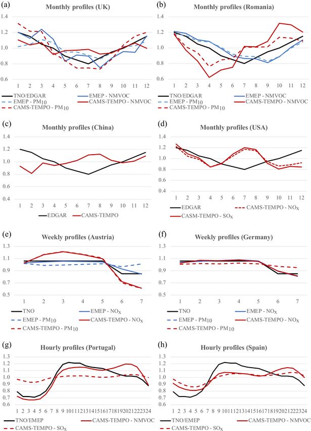
374                                                                                                     M. Guevara et al.: CAMS-TEMPO

Figure 1. Representation of the spatial coverage of the datasets used to derive temporal profiles for the energy industry (a), the manu-
facturing industry (b), road transport (c) and agriculture (use of fertilizers) (d). For the energy industry, the legend indicates the different
sources of information used: the European Network of Transmission System Operators for Electricity (ENTSO-E), the United States En-
vironmental Protection Agency (US EPA), the International Energy Agency (IEA) and the Monthly Bulletin of Statistics (MBS). For the
manufacturing industry, the legend indicates the sources of information used: the MBS and the MIX inventory (mosaic Asian anthropogenic
emission inventory, Li et al., 2017). For agriculture, sources of information are also highlighted: Backes et al. (2016), Zhang et al. (2018), the
MASAGE_NH3 (Magnitude And Seasonality of Agricultural Emissions model for NH3 ) inventory (Paulot et al., 2014), US EPA (2019b),
Skjøth et al. (2011) and Werner et al. (2015). Administrative boundaries are derived from GADM (2020).

Table 4. Emission factors [kg TJ−1 ] related to the energy industry per fuel type and pollutant. Values obtained from the EMEP/EEA 2016
emission inventory guidebook for the priority air pollutants (1.A.1 “Energy industries”, Tables 3-2, 3-3, 3-4, 3-5 and 3-7) and from the IPCC
guidelines (Volume 2: “Energy”, Table 2.2) for greenhouse gases.

                   Fuel and EF [kg TJ−1 ]          NOx      SOx       CO     NMVOC         PM10    PM2.5         CO2     CH4
                   Hard coal                        209      820      8.7            1.0     7.7      3.4      98 300        1
                   Brown coal (lignite)             247    1680       8.7            1.4     7.9      3.2     101 000        1
                   Gaseous fuels (natural gas)       89    0.281       39            2.6    0.89     0.89      56 100        1
                   Heavy fuel oil                   142      495     15.1            2.3    25.2     19.3      77 400        1
                   Biomass                           81     10.8      90            7.31    155      133      112 000       30

emissions reported by the EPA’s CEMS data. Measurements                     type of power plant. Pollutant-related weekly profiles were
from all individual plants were averaged at the monthly level               developed following the same methodology applied for ob-
and then normalized to sum 12. The seasonality for the other                taining the monthly weight factors (Eq. 1).
pollutants (i.e. NMVOC, NH3 , CO, PM10 , PM2.5 , CO2 and                       For the US, the CEMS data were used to compute
CH4 ) was linked to the measured heat input, following Stella               pollutant-dependent profiles following the same procedure
(2005).                                                                     as described in Sect. 2.2.1. Measurements from all individ-
                                                                            ual plants were averaged per day of the week and then nor-
2.2.2   Weekly profiles                                                     malized to sum 7. For countries with no information on daily
                                                                            electricity production data, we used the weekly profile re-
Weekly profiles were developed for Europe using the hourly                  ported in the TNO dataset for the energy sector.
electricity production data reported by ENTSO-E. As in
the case of the monthly profiles, weekly scale factors were                 2.2.3     Hourly profiles
found to significantly vary according to the type of fuel
(Fig. S1). These results are in line with the conclusions of                Hourly profiles were developed for Europe and the US using
Adolph (1997), which identified three generic weekly pro-                   the hourly electricity production data reported by ENTSO-E
files – base, medium and peak load – as a function of the                   and the measured emissions reported by CEMS, respectively.

Earth Syst. Sci. Data, 13, 367–404, 2021                                                       https://doi.org/10.5194/essd-13-367-2021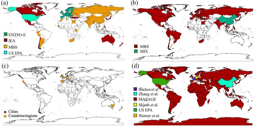
M. Guevara et al.: CAMS-TEMPO                                                                                                  375

As previously seen, large differences are observed between         (C3S, 2017). As shown in Eq. (2), HDD (x, d) increases with
fuels. Profiles related to the so-called base peak load power      the difference between the threshold and actual outdoor tem-
plants (i.e. annual useful life of more than 4000 h) present a     peratures. A minimum value of 1 is assumed instead of 0 to
rather flat distribution, whereas in other cases the change in     avoid numerical problems when used in Eq. (3).
energy production between day and night is relatively high            A challenge when using this method is to set the thresh-
(Fig. S1).                                                         old or comfort temperature (Tb ). The choice of Tb depends
   Pollutant-related hourly profiles were developed follow-        on local climate and building characteristics, among others.
ing the same procedure shown in Eq. (1). For countries with        When dealing with an extended area like Europe or even
no information on hourly electricity production data, we as-       the whole world, it is difficult to choose a unique Tb . This
sumed the hourly profile reported in the TNO dataset. Some         value is usually set to 18 ◦ C (e.g. Mues et al., 2014), 15.5 ◦ C
studies have suggested that the hourly variation of power          (e.g. Spinoni et al., 2015) or even 15 ◦ C (e.g. Stohl et al.,
plant activities may vary according to the season of the year      2013). Following the work by Spinoni et al. (2015), which
(Thiruchittampalam, 2014). This feature is not considered in       developed gridded European degree-day climatologies, we
the present version of the CAMS-TEMPO profiles and will            assumed that Tb = 15.5 ◦ C, a value also suggested by the
be addressed in future releases.                                   UK Met Office. A first guess of the daily temporal factor
                                                                   (FD (x, d)) for grid cell x and day d is (Eq. 3)
2.3     Residential and commercial combustion
                                                                                 HDD (x, d)
                                                                   FD (x, d) =              ,                                   (3)
The temporal profiles computed for the residential and com-                       HDD (x)
mercial sector are reported under the res sector in CAMS-
GLOB-TEMPO and the GNFR_C category in CAMS-REG-                    where HDD (x) is the yearly average of the heating-degree-
TEMPO. The temporal variability of emissions for this sec-         day factor per grid cell x (Eq. 4),
tor is assumed to be dominated by the stationary combustion                      PN
of fossil fuels in households and commercial and public ser-                       1   HDD (x, d)
                                                                   HDD (x) =                      ,                             (4)
vice buildings. These categories are also assumed to be the                             N
main contributors to the total emissions reported by CAMS-
                                                                   where N = 365 or 366 d (leap or non-leap year). Consider-
GLOB-ANT and CAMS-REG_AP/GHG. Other combustion
                                                                   ing that residential combustion processes are related not only
installations activities included under this sector (i.e. plants
                                                                   to space heating but also to other activities that remain con-
in agriculture, forestry and aquaculture and other stationary
                                                                   stant throughout the year such as water heating or cooking, a
facilities including military) are assumed to follow the same
                                                                   second term is introduced to Eq. (5) by means of a constant
temporal profile.
                                                                   offset (f ) (Eq. 5):
   The temporal weight factors developed for this sector in-
clude monthly, daily and hourly profiles. The monthly and                        HDD (x, d) + f · HDD (x)
daily profiles depend upon year and region and were de-            FD (x, d) =                            ,                     (5)
rived using meteorological parametrizations (Sect. 2.3.1).                         (1 + f ) · HDD (x)
The hourly profiles depend upon pollutant and region               where f = 0.2 based on the European household energy
(Sect. 2.3.2).                                                     statistics reported by Eurostat (2018) (Table 5). As observed,
                                                                   this share may vary depending on fuel. In the case of biofuels
2.3.1    Monthly and daily profiles                                or coal products, which dominate the contribution to total PM
                                                                   emissions, space heating represents 89.1 % of the residential
Gridded daily temporal profiles were derived according to
                                                                   combustion processes (f ∼ 0.1), whereas in the case of nat-
the heating-degree-day (HDD) concept, which is an indicator
                                                                   ural gas, which is the main contributor to NOx , the share is
used as a proxy variable to reflect the daily energy demand
                                                                   77.7 % (f ∼ 0.2). Significant differences between countries
for heating a building (Quayle and Diaz, 1980). This method
                                                                   are also observed for specific fuels. For instance, in Nor-
has been proven to be successful in previous emission mod-
                                                                   way 100 % of solid fuels are used for space heating (f ∼ 0),
elling work (e.g. Mues et al., 2014; Terrenoire et al., 2015).
                                                                   whereas in Greece this share is only 65 % (f ∼ 0.35), with
   The heating-degree-day factor (HDD (x, d)) for grid cell
                                                                   the remainder being attributed to water heating (27 %) and
x and day d is defined relative to a threshold temperature
                                                                   cooking (8 %) (Eurostat, 2018). More significant differences
(Tb ), above which a building needs no heating (i.e. heating
                                                                   can be found in developing regions (e.g. Tibetan Plateau),
appliances will be switched off), following Eq. (2):
                                                                   where the share of solid biofuels used for cooking can go up
HDD (x, d) = max(Tb − T2 m (x, d) , 1),                     (2)    to 80 %. Despite these variations, a generic value of f = 0.2
                                                                   is assumed for all regions. To illustrate how current assump-
where T2 m (x, d) is the daily mean 2 m outdoor temperature        tions may impact the derived profiles in non-European re-
for grid cell x and day d [◦ C]. This information was obtained     gions, we computed daily factors for the residential sector
from the ERA5 reanalysis dataset for the period 2010–2017          over India and China for 2015 using a range of f (0, 0.2

https://doi.org/10.5194/essd-13-367-2021                                               Earth Syst. Sci. Data, 13, 367–404, 2021
376                                                                                          M. Guevara et al.: CAMS-TEMPO

and 0.5) and Tb (15.5 and 18 ◦ C) values (Fig. S2). We se-
lected these two countries, as they produce a large share of
the global residential emissions (Hoesly et al., 2018). Differ-
ences between the daily factors of up to 55 % were found dur-
ing wintertime when comparing the results computed with
f = 0.0 and 0.5, indicating that daily factors are sensitive to
these parameters. The investigation and proposal of different
f values (as well as different Tb values) for different regions
of the world will be addressed in future work.
   Gridded daily temporal profiles were developed for 8 years
(2010 to 2017). A climatological daily profile based on the
average of each day over all the available years was also
produced. Monthly gridded factors were derived from the
daily profiles for all the years available. We interpolated
the estimated gridded daily factors from the ERA5 work-
ing domain (approx. 0.3×0.3◦ ) onto the CAMS-GLOB-ANT
(0.1 × 0.1◦ ) and CAMS-REG_AP/GHG (0.05 × 0.1◦ ) grids,
applying a nearest-neighbour approach.

2.3.2   Hourly profiles

The hourly distribution of residential and commercial com-
bustion activities has typically been described following
the profile A presented in Fig. 2a, used in both EMEP
                                                                  Figure 2. (a) Proposed hourly temporal profiles for the residential
and TNO datasets. This hourly distribution presents one
                                                                  and commercial combustion sector where profile A refers to NOx,
peak in the morning and another one in the afternoon,             SOx and CH4 emissions in urban and rural areas of developed and
when energy consumption is supposedly higher due to               developing countries; profile B refers to PM10 , PM2.5 , CO, CO2 ,
increased space heating or cooking activities. We eval-           NMVOC and NH3 in urban and rural areas of developed countries;
uated this profile with real-world measurements of nat-           and profile C refers to all pollutants in rural areas of developing
ural gas consumption for residential houses in the UK             countries. (b) Comparison between the hourly temporal profile pro-
(Retrofit for the Future project, https://www.ukgbc.org/          posed by TNO for agricultural emissions (Denier van der Gon et
ukgbc-work/retrofit-for-the-future-innovate-uk/, last access:     al., 2011) and the three measurement-based temporal profiles re-
February 2021) and the US state of Texas (Data Port – Pecan       ported by Walker et al. (2013) derived from NH3 flux measurements
Street dataset, https://dataport.cloud/, last access: Febru-      performed in a fertilized corn canopy in North Carolina, James et
ary 2021) and a house in Canada (Makonin et al., 2016).           al. (2012) based on direct NH3 measurements performed in a me-
                                                                  chanically ventilated swine barn and Mu et al. (2011) derived from
The measurements show the two peaks in all the profiles,
                                                                  active fire satellite observations.
although their occurrence and intensity vary due to the spe-
cific energy consumption behaviour of each house (Fig. S2).
This comparison suggests that profile A is representative of
emissions related to natural gas combustion.                      2013). We created a third profile that represents these activ-
   We created a second hourly profile (Fig. 2a, profile B)        ities (Fig. 2a, profile C) based on information derived from
linked to the combustion of residential wood for space-           continuous indoor PM2.5 measurements performed in house-
heating purposes using as a basis information derived from        holds in the eastern Tibetan Plateau (Carter et al., 2016).
citizen interviews performed in Norway and Finland (Finstad       The profile is influenced by heating and cooking practices
et al., 2004 and Gröndahl et al., 2010) as well as from long-     and therefore presents three peaks that correspond to typical
term measurements of the wood-burning fraction of black           morning, midday and evening mealtimes.
carbon in Athens (Athanasopoulou et al., 2017). As shown in          The results summarized in Fig. 2a indicate that the hourly
Fig. 2a, the resulting profile B presents an intense peak dur-    behaviour of residential combustion emissions varies accord-
ing the evening hours, but not during the morning, in contrast    ing not only to the fuel type but also to the type of end use
to profile A. It is actually a common practice in developed       (i.e. space heating or cooking). Both CAMS-GLOB-ANT
countries to use fireplaces and other types of wood-burning       and CAMS-REG_AP/GHG report total residential and com-
appliances mainly in the evening.                                 mercial emission as a unique sector, without discriminating
   As reported by the World Health Organization (WHO),            by type of fuel or end use. Therefore, several decisions were
most developing countries use wood not only for heating           made in order to assign the three proposed profiles to differ-
space purposes but also for cooking activities (Bonjour et al.,   ent pollutants and regions:

Earth Syst. Sci. Data, 13, 367–404, 2021                                            https://doi.org/10.5194/essd-13-367-2021
M. Guevara et al.: CAMS-TEMPO 377
– profile A: NOx , SOx and CH4 emissions in urban and monthly evolution of the productive activity of different in-
rural areas of developed and developing countries; dustrial branches, including manufacturing activities. The IPI
as a monthly surrogate for industrial emissions has been used
– profile B: PM10 , PM2.5 , CO, CO2 , NMVOC and NH3 in previous studies (e.g. Pham et al., 2008; Markakis et al.,
in urban and rural areas of developed countries; and 2010).
The IPI data were obtained from the MBS database (MBS,
– profile C: all pollutants in rural areas of developing
2018), which provides monthly information per country and
countries.
general industrial branch (i.e. mining, manufacturing, elec-
The assumptions made behind this assignment are the fol- tricity, gas and steam, and water supply) for the year 2015.
lowing: The manufacturing branch, which includes several divisions
such as iron and steel industries, chemical industries, and
– Natural gas and diesel heating combustion is the main food and beverage products, was used to derive country-
contributor to total NOx , SOx and CH4 emissions. specific monthly profiles. Figure 1b shows the spatial cov-
erage of the compiled dataset. As in the case of the energy
– Wood combustion is the main contributor to total PM10 ,
industry sector (Fig. 1a), the lack of information mostly af-
PM2.5 , CO, CO2 , NMVOC and NH3 emissions.
fects Africa and South America. For those countries with-
– In the urban and rural areas of developed countries out available information, the monthly profile reported in the
wood is mainly used for heating purposes. TNO dataset under the industry sector was used (Denier van
der Gon et al., 2011). In the case of China, the monthly pro-
– In the urban areas of developing countries wood is file reported in the MIX inventory under the industry sector
mainly used for heating purposes. was used (Li et al., 2017).
The time profiles are based on IPI information from 2015
– In the rural areas of developing countries all fuels are and are assumed to be representative for other years. Our as-
used both for heating and/or cooking purposes (i.e. the sumption is supported by the low interannual variability ob-
two activities occur at the same time). served in the IPI values collected from different national sta-
The list of developing countries was obtained from the World tistical offices including Italy (ISTAT, 2018), Norway (SSB,
Bank country classifications (World Bank, 2014). The dis- 2018), Spain (INE, 2018) and the UK (ONS, 2018) (Fig. S3).
crimination of human settlements between urban and ru- Another implicit assumption made is that the constructed
ral areas was derived from the Global Human Settlement monthly profiles can be equally applied to all the different
Layer (GHSL) project (Florczyk et al., 2019; Pesaresi et industrial activities reported under the ind and GNFR_B sec-
al., 2019). The GHSL provides a global classification of tors. The national IPI values collected for Italy and the US
human settlements on the basis of the built-up settlement (Board, 2020) were used to compare the seasonality of indi-
and population density at a resolution of 1 km × 1 km cor- vidual industrial divisions to the general manufacturing IPI
responding to four epochs (2015, 2000, 1990 and 1975). monthly profile. For both countries, as well as up to a certain
The 2015 epoch was selected, and the original raster was extent, it was found that all the industrial divisions (except
remapped onto the CAMS-GLOB-ANT (0.1 × 0.1◦ ) and food and beverages and the petrochemical industry in the
CAMS-REG_AP/GHG (0.1 × 0.05◦ ) grids. case of Italy) follow the seasonality of the general manufac-
turing profile (Fig. S4), which allows for concluding that the
assumption made is reasonable. A similar result is reported
2.4 Manufacturing industry
for Thailand in Pham et al. (2008).
The temporal variability of industrial emissions is re-
ported under the sectors indu (CAMS-GLOB-TEMPO) 2.4.2 Weekly and hourly profiles
and GNFR_B (CAMS-REG-TEMPO). Both in the CAMS-
GLOB-ANT and the CAMS-REG_AP/GHG inventories, all Due to the lack of country-specific data, the fixed weekly
industrial manufacturing emissions are reported under these and hourly temporal profiles provided in the TNO dataset for
single categories. Hence, the same temporal pattern has to be industry sector are used. The weekly profile assumes a flat
assumed for all types of facilities (e.g. cement plants, iron distribution during the working days and a slight decrease
and steel plants, and food and beverage). For this sector, only during weekends (Table A2). On the other hand, the hourly
country-dependent monthly profiles were developed due to profile includes an increase of the activity during the central
the lack of more detailed data. hours of the day (Tables A3 and A4).
2.4.1 Monthly profiles 2.5 Road transport
Country-specific monthly profiles were estimated using Temporal profiles for road transport emissions are reported
the Industrial Production Index (IPI), which measures the under the tro sector in CAMS-GLOB-TEMPO and the
https://doi.org/10.5194/essd-13-367-2021 Earth Syst. Sci. Data, 13, 367–404, 2021378 M. Guevara et al.: CAMS-TEMPO
Table 5. Share of final energy consumption in the residential sector by fuel and type of end use in Europe (Eurostat, 2018).
Fuel Space heating Water heating Cooking Other end uses
Gas 77.7 % 17.2 % 5.1 % –
Solid fuels (coal products) 90.7 % 8.2 % 1.1 % –
Petroleum products (LPG and fuel oil) 81.1 % 12.9 % 6.0 % 0.1 %
Renewables and wastes (solid biofuels) 89.1 % 8.8 % 1.7 % 0.4 %
All 81.8 % 13.9 % 4.2 % 0.1 %
GNFR_F1 (exhaust gasoline), GNFR_F2 (exhaust diesel), urday) profiles were constructed (Fig. S5). The results sug-
GNFR_F3 (exhaust LPG gas) and GNFR_F4 (non-exhaust) gest that temporal patterns in vehicle activity do not change
categories in CAMS-REG-TEMPO. The fact that CAMS- much over long timescales. Consequently and following the
REG_AP/GHG traffic-related emissions are classified into assumptions made for the energy and manufacturing indus-
four different categories (discriminated by fuel and type of try sectors, we assumed that the interannual variability can
process) allows for considering specific temporal features as- be negligible. Hence, all profiles developed only as a func-
sociated with each one of them, including temperature de- tion of traffic count data were constructed by averaging the
pendence of CO and NMVOC gasoline exhaust emissions values (per month, day of the week or hour of the day) over
(GNFR_F1), of NOx diesel exhaust emissions (GNFR_F2) all the available years.
and of NMVOC non-exhaust emissions (GNFR_F4). On the Some of the compiled datasets (e.g. Germany and Cal-
other hand, in CAMS-GLOB-ANT all traffic emissions are ifornia) report the traffic counts classified by vehicle type
reported under a single sector, and subsequently the approach (i.e. light-duty vehicles, LDVs, and heavy-duty vehicles,
used for the development of the temporal profiles is more HDVs). The monthly, weekly and hourly profiles as a func-
simplistic. tion of the vehicle type showed significant differences, espe-
The temporal weight factors developed for this sector in- cially for weekly and hourly profiles (Fig. S6). HDV traffic
clude monthly, weekly and hourly profiles. As summarized presents a larger decrease on the weekend than LDV traf-
in Table 2, the CAMS-GLOB-TEMPO monthly and weekly fic. Moreover, the hourly LDV profile exhibits two distinct
profiles constructed for this sector are region-dependent, (morning and evening) commuter-related peaks, whereas
whereas the hourly profiles vary per region and day of HDV shows a single midday peak. These results highlight
the week (i.e. weekday, Saturday and Sunday). In the case the importance of applying separate temporal profiles to
of CAMS-REG-TEMPO, the constructed profiles can vary characterize traffic and associated emissions for LDVs and
by region, pollutant, day of the week and/or year, as a HDVs. However, in the present work this disaggregation
function of the source sector and temporal resolution (Ta- was not considered, since both the CAMS-GLOB-ANT and
ble 3). Depending on the dataset and sector category, tem- CAMS-REG_AP/GHG inventories report LDV- and HDV-
poral emission variability is assumed to be either exclusively related emissions under the same pollutant sector. When only
driven by the traffic activity data (e.g. CAMS-GLOB-TEMP, vehicle-type temporal profiles were available (i.e. Califor-
all cases) or by a combination of traffic activity data and nia), the information reported for LDVs is used, as this type
changes in ambient temperature (i.e. CAMS-REG-TEMP, of vehicle dominates the temporal distribution of total traffic
CO and NMVOC GNFR_F1, NOx GNFR_F2, and NMVOC flow.
GNFR_F3). For the first case, temporal profiles were devel-
oped using traffic count data compiled from multiple sources
2.5.1 Meteorology-independent monthly profiles
of information (Sect. 2.5.1). As listed in Table 6, the in-
formation was obtained from local and national open-data A comparison between monthly variation in traffic patterns
portals, publications or through personal communications. at urban and rural locations (i.e. urban streets and high-
The spatial coverage of the compiled dataset is illustrated in ways) was performed for selected countries or regions in-
Fig. 1c. For the second group of profiles, the temporal vari- cluding California, Germany, Spain and the UK. For the UK
ability of traffic activity was combined with meteorological and California, the original traffic statistics were already dis-
parametrizations available in the literature (Sect. 2.5.2). criminated by type of location. For the German and Spanish
Considering that for each traffic count dataset the refer- datasets, each traffic station was classified as urban or rural
ence years are different (Table 6), we analysed the data in considering its geographical location and the GHSL human
view of differences in the resulting profiles as a function of settlement classification dataset (Sect. 2.3.2). As shown in
the year. We took the Paris city traffic data as an example, Fig. 3, while there is little seasonal variation in German ur-
since it covers a wide range of years (2013 to 2017). For each ban locations, rural areas tend to exhibit a stronger seasonal-
year, monthly, weekly and hourly (i.e. Wednesday and Sat- ity, with a peak occurring during summertime, presumably
Earth Syst. Sci. Data, 13, 367–404, 2021 https://doi.org/10.5194/essd-13-367-2021You can also read