DESIGN OF A CODE-AGNOSTIC DRIVER APPLICATION FOR HIGH-FIDELITY COUPLED NEUTRONICS AND THERMAL-HYDRAULIC SIMULATIONS
←
→
Page content transcription
If your browser does not render page correctly, please read the page content below
EPJ Web of Conferences 247, 06053 (2021)                                                               https://doi.org/10.1051/epjconf/202124706053
PHYSOR2020

                  DESIGN OF A CODE-AGNOSTIC DRIVER APPLICATION FOR
                       HIGH-FIDELITY COUPLED NEUTRONICS AND
                          THERMAL-HYDRAULIC SIMULATIONS

                    Paul K. Romano1 , Steven P. Hamilton2 , Ronald O. Rahaman1 , April Novak3 ,
                           Elia Merzari1 , Sterling M. Harper4 , and Patrick C. Shriwise1
                                            1
                                              Argonne National Laboratory
                                    9700 S. Cass Ave., Lemont, IL 60439, USA
                                                        2
                                                   Oak Ridge National Labroatory
                                          1 Bethel Valley Rd., Oak Ridge, TN 37831, USA
                                                    3
                                                 University of California-Berkeley
                                          3115 Etcheverry Hall, Berkeley, CA 94708, USA
                                                4
                                              Massachusetts Institute of Technology
                                       77 Massachusetts Ave., Cambridge, MA 02139, USA

                   promano@anl.gov, hamiltonsp@ornl.gov, rahaman@anl.gov, novak@berkeley.edu
                           ebm5351@psu.edu, smharper@mit.edu, pshriwise@anl.gov

                                                                  ABSTRACT

               While the literature has numerous examples of Monte Carlo and computational fluid dy-
               namics (CFD) coupling, most are hard-wired codes intended primarily for research rather
               than as standalone, general-purpose codes. In this work, we describe an open source
               application, ENRICO, that allows coupled neutronic and thermal-hydraulic simulations
               between multiple codes that can be chosen at runtime (as opposed to a coupling between
               two specific codes). In particular, we outline the class hierarchy in ENRICO and show
               how it enables a clean separation between the logic and data required for a coupled sim-
               ulation (which is agnostic to the individual solvers used) from the logic/data required for
               individual physics solvers. ENRICO also allows coupling between high-order (and gen-
               erally computationally expensive) solvers to low-order “surrogate” solvers; for example,
               Nek5000 can be swapped out with a subchannel solver.
               ENRICO has been designed for use on distributed-memory computing environments. The
               transfer of solution fields between solvers is performed in memory rather than through file
               I/O. We describe the process topology among the different solvers and how it is leveraged
               to carry out solution transfers. We present results for a coupled simulation of a single
               light-water reactor fuel assembly using Monte Carlo neutron transport and CFD.

         KEYWORDS: Monte Carlo, CFD, multiphysics, nuclear reactor, open source

  © The Authors, published by EDP Sciences. This is an open access article distributed under the terms of the Creative Commons Attribution License 4.0
  (http://creativecommons.org/licenses/by/4.0/).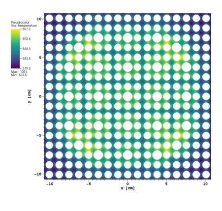
EPJ Web of Conferences 247, 06053 (2021)                                        https://doi.org/10.1051/epjconf/202124706053
PHYSOR2020

                                               1. INTRODUCTION

         The analysis of nuclear reactors requires the simultaneous solution of multiple equations represent-
         ing different physical phenomena: neutral particle transport, fluid dynamics, heat transfer, material
         burnup, and possibly others. Consequently, simulations of multiple physics fields, or multiphysics
         simulations, have become commonplace in reactor analysis. Recent research efforts have focused
         on improving the accuracy of coupled solutions by employing the most accurate methods for in-
         dividual physics fields, namely, the Monte Carlo (MC) method for neutral particle transport and
         computational fluid dynamics (CFD). While the use of these methods for multiphysics simula-
         tions has historically been limited by available computational resources, continued improvements
         in CPU performance may make such calculations feasible to carry out in a shorter time and for
         larger systems.

         In this paper, we report on a new application designed to carry out coupled MC and CFD calcula-
         tions. The idea of coupling existing MC and CFD codes is not new, and multiple researchers have
         demonstrated such couplings using a variety of codes over the past 13 years [1–13]. While we will
         not attempt to discuss in detail each of these prior works, we will mention a few themes that appear
         across them that limit their generality. To begin with, many of these works were one-off studies
         that were not intended to be used by a broader user community. As a result, the methodology
         employed for coupling the codes was often inherently limited. For example, in many works, the
         coupling between the MC and CFD solvers was done through filesystem I/O rather than directly
         in memory. More importantly, the mapping of solutions between solvers was done manually in
         many instances rather than in an automated fashion. Other issues that can be observed in the lit-
         erature include the lack of automated convergence checks, instead relying on a maximum number
         of Picard iterations, and the lack of under-relaxation, which can potentially lead to oscillatory or
         divergent solutions.

         For coupled MC and CFD calculations to become attractive and useful to a wider community of
         engineers and researchers, code systems for performing such calculations need to developed that
         are accurate, robust, and sufficiently general. Of the above mentioned works, only the coupling
         between Serpent 2 and OpenFOAM [12] appears to be a production capability that is available
         as a general feature to users. In this case, the use of an unstructured mesh overlaid on top of the
         MC constructive solid geometry model along with delta tracking allows solutions to be transferred
         between solvers without needing to perform any interpolation; for example, changes in temperature
         and density need not occur only at material boundaries in the MC model.

         Under the DOE Exascale Computing Project, we are developing capabilities for coupled MC and
         CFD simulations on future exascale supercomputing architectures, including GPUs [14]. At the
         onset of development, we defined a number of requirements that the driver application would need
         to satisfy:

         • The driver must have the ability to call solvers and obtain solutions directly in memory, as
           opposed to going through a filesystem.
         • In addition to calling the application codes, the driver should have the ability to use simplified
           “surrogate” solvers for each physics field to quickly iterate between a single high-fidelity solver
           and the surrogate solver and for debugging, testing, and verification purposes.

                                                          2
EPJ Web of Conferences 247, 06053 (2021)                                         https://doi.org/10.1051/epjconf/202124706053
PHYSOR2020

         • Because this work involves multiple laboratories and MC codes (Shift and OpenMC), the driver
           application should be able to couple solvers in a manner that is agnostic to the actual code used.
         • To encourage external use and contributions to the driver application, the application should be
           made publicly available through an open source license.

         The code that we have developed, ENRICO (Exascale Nuclear Reactor Investigative COde), is to
         our knowledge the first such general code geared toward coupled neutronic and thermal-hydraulic
         calculations that meets these constraints. Qiu et al. describe a multiphysics coupling system de-
         signed for fusion energy applications that appears to be capable of handling multiple MC and CFD
         codes [15]; however, the coupling is done only in one direction, with the heat source from the MC
         code used as a source in the CFD solve. Data transfers were also done through file I/O rather than
         in memory. Moreover, the code system does not appear to have been made generally available.

         The remainder of the paper is organized as follows. Section 2 describes the design and implemen-
         tation of ENRICO. Section 3 describes results of a coupled simulation of OpenMC and Nek5000
         using ENRICO on a full-length pressurized water reactor (PWR) fuel assembly problem. Section 4
         concludes the paper by discussing the work accomplished to date and avenues for future work.

                                               2. METHODOLOGY

         Because of the nature of the solvers being used, one cannot have a tightly coupled code wherein
         all fields are solved for simultaneously. Thus, ENRICO is designed to iteratively solve for the
         different physics fields using a Picard iteration as in most prior works. The primary application
         codes that have initially been included are the OpenMC and Shift MC codes and the Nek5000
         spectral element CFD code. OpenMC and Shift are both written in C++14, and Nek5000 is written
         in Fortran. OpenMC and Shift can both be built as shared libraries and expose a C/C++ API
         that can be used to make geometry queries, create new tallies, obtain tally results, and perform
         basic execution (initialization, running a transport solve, resetting state, finalizing). For Nek5000,
         slightly more effort was required to achieve an in-memory coupling; a thin C API was developed
         that exposes the basic queries needed for coupling, namely, determining element centroids and
         temperatures and setting a heat source.

         In order to simplify the coupling, a number of assumptions were made regarding how the models
         are constructed:

         • The boundaries of cells in the MC constructive solid geometry model are exactly aligned with
           the boundaries of elements in the CFD model. If this assumption is violated, a discretization
           error may be present in the solution (which may or may not be acceptable depending on the
           discretization). Note that because spectral elements can have curvature along their edges, exact
           alignment is possible when coupling with Nek5000.
         • Each cell in the neutronic model contains one or more spectral elements. That is to say, the CFD
           discretization is finer than the MC discretization.
         • While Nek5000 normally operates on nondimensionalized quantities, the actual units are impor-
           tant for coupling. Our driver assumes that the Nek5000 model has been set up such that lengths
           are in [cm], temperatures are in [K], and the heat source can be given in [W/cm3 ].

                                                          3
EPJ Web of Conferences 247, 06053 (2021) https://doi.org/10.1051/epjconf/202124706053
PHYSOR2020
To satisfy these assumptions requires coordinated efforts by whomever creates models for the
individual codes.
2.1. Flow of Execution
At the beginning of a simulation, each solver must be initialized to read input files, setup necessary
data structures, and so forth. Once the solvers are initialized, a mapping between the particle
transport and heat/fluid solvers is established. The interface to each heat/fluid solver has a function
that returns a centroid for each element. These point locations are then used in the particle transport
solver to determine what cells contain the given locations. Two mappings are stored: one that gives
a list of heat/fluid elements for each cell and one that gives a cell for each heat/fluid element. By
establishing this mapping at runtime, the user of the driver application need not manually establish
a mapping between the solvers. This approach is identical to that described by Remley et al. [11].
After the mapping between particle transport and heat/fluid regions has been established, the driver
creates tallies for energy deposition in each cell that contains a heat/fluid element. While we are
currently assuming that energy deposition occurs only in the fuel pin, this assumption may be
relaxed further along in the project to account for energy deposition in the fluid from neutron
elastic scattering and energy deposition in structural materials from photon heating.
With the necessary tallies set up, the driver begins by executing the particle transport solver to
obtain energy deposition in each cell, qi . The energy deposition returned by the particle transport
solver is in units of [J/source] and has to be normalized to the known power level of the reactor, Q̇,
in [W]. Dividing the power level by the sum of the energy deposition rates gives us a normalization
factor:
Q̇ [W] source
f= = = . (1)
qi [J/source] s
i
Multiplying qi by the normalization factor and dividing by the volume of the cell, we get a volu-
metric heat generation rate:
f qi [source/s] [J/source] W
qi = = = . (2)
Vi [cm3 ] cm3
With the volumetric heat generation rate determined, the driver updates the source for the energy
equation in the heat/fluid solver by applying the heat generation rate qi to any heat/fluid elements
that are contained within cell i (utilizing the mapping that is established at initialization). The
heat/fluid solver is then executed to obtain temperatures and densities in each heat/fluid element.
For each cell, an average temperature is obtained by volume-averaging the temperatures within
each heat/fluid element in the cell. If the heat/fluid solver provides a density on each element, a
volume-averaged density in each cell can also be obtained. However, some formulations of the
conservation equations do not require density; in this case, the density must be obtained through a
closure relation that gives the density or specific volume as a function of pressure and temperature.
Once these volume-averaged temperatures and densities are obtained, they are applied as updates
in the particle transport solver, and the Picard iteration is complete.
4EPJ Web of Conferences 247, 06053 (2021) https://doi.org/10.1051/epjconf/202124706053
PHYSOR2020
Convergence of the Picard iteration can be handled in two ways. The user can select a maximum
number of Picard iterations to be performed. Alternatively, the user can specify a tolerance, , on
the L1 , L2 , or L∞ norm of the temperature at each iteration. This requires storing the temperature
within each element at both the current and previous iteration. In other words, if Ti is a vector of
the temperatures within each element at Picard iteration i, convergence is reached if
Ti − Ti−1 < , (3)
where the norm depends on the user’s selection. While it would be more robust to check the
difference for all coupled fields (temperature, density, and heat source), previous studies have
demonstrated that checking the temperature alone is usually sufficient. Note that by storing the
temperature (and heat source) at two successive iterations, under-relaxation can be performed dur-
ing the temperature or heat source update.
2.2. Driver Class Design
At the top of the class hierarchy, shown in Fig. 1, is a CoupledDriver class that controls the
execution of the entire simulation. The CoupledDriver class holds most of the important state,
including pointers to neutronics and heat-fluids driver base classes and values for the temperature,
density, and heat source at the current and previous Picard iteration. Other attributes that are stored
on the CoupledDriver class but not shown in Fig. 1 include the mappings between cells in the
MC code and elements in the CFD code, initial/boundary conditions, and parameters for under-
relaxation.
CoupledDriver NeutronicsDriver OpenmcDriver
-neutronics_driver_: NeutronicsDriver +find()
-heat_fluids_driver_: HeatFluidsDriver +create_tallies()
-temperature_: Array[double] +solve_step() ShiftDriver
-temperature_prev_: Array[double] +heat_source()
-density_: Array[double] +set_temperature()
-density_prev_: Array[double] +set_density()
-heat_source_: Array[double] +get_density()
-heat_source_prev_: Array[double] +get_temperature()
+... +get_volume()
+is_converged() +is_fissionable()
+update_heat_source()
+update_temperature() HeatFluidsDriver NekDriver
+update_density()
+solve_step()
+set_heat_source_at()
+centroid_local() SurrogateHeatDriver
+volume_local()
+temperature_local()
+density_local()
+centroids()
+volumes()
+temperature()
+density()
Figure 1: Class hierarchy for driver classes in ENRICO.
The NeutronicsDriver and HeatFluidsDriver classes are abstract base classes that de-
fine the required interfaces that concrete classes must implement. Currently, NeutronicsDriver
has two implementations: OpenmcDriver and ShiftDriver. HeatFluidsDriver also
has two implementations: NekDriver and SurrogateHeatDriver, the latter of which im-
plements a basic subchannel solver in the fluid and a 1D cylindrical finite-difference heat diffusion
solver in the fuel with radiative heat transfer in the gap. Because it is not the main focus of this
5EPJ Web of Conferences 247, 06053 (2021) https://doi.org/10.1051/epjconf/202124706053
PHYSOR2020
paper, we will not discuss the surrogate solver in detail but rather just mention that it can be used
to debug the overall coupled simulation by providing an approximate solution.
By storing the simulation state in the CoupledDriver class, most of the logic for execution is
also contained in the coupled driver class, such as establishing the code-to-code domain mappings,
controlling the overall coupled Picard iteration, calculating under-relaxed solution fields, and per-
forming convergence checks. Adding another individual physics solver in the system entails cre-
ating a concrete implementation of one of the abstract classes, either NeutronicsDriver or
HeatFluidsDriver.
2.3. Parallel Execution and Data Transfer Mechanics
Both the CFD and MC solvers potentially require significant computational resources and will
each use a parallel solution approach. Nek5000 uses a standard domain decomposition approach
in which the global problem is distributed among a number of processors (MPI ranks). OpenMC
and Shift typically use a domain replicated approach in which the problem domain is replicated on
all processors and the total number of particle histories to be simulated is distributed among the
processors. Although Shift supports a combination of domain replication and domain decomposi-
tion, for this study it is being used only with domain replication.
In the current implementation, the CFD and MC solvers are each assigned to execute on all avail-
able processors. The solvers must therefore share resources (e.g., memory) on each processor. This
approach may be problematic for problems where both physics solvers have substantial resource
requirements. In a variant of this approach, the MC solver may be assigned to the same compute
nodes as the CFD solver but only a subset of the MPI ranks of the global communicator (frequently
one rank per node). This setup allows the MC solver to use shared-memory parallelism within a
node and domain replication across nodes. Although the use of shared-memory parallelism re-
duces the overall memory footprint of the MC solver, the CFD and MC solvers must still share the
available resources on a node. In this approach, the physics solvers can alternate execution during
a multiphysics calculation, with one solver having dedicated use of all processors during its solve.
As noted in Section 2.1, temperature and fluid density information must be transferred from the
CFD solver to the MC solver, and the heat generation rate must be transferred from the MC solver
to the CFD solver. Temperature/density information stored on the CFD mesh must be averaged
onto MC geometric cells, and heat generation information on the MC geometry must be distributed
to the corresponding CFD elements. Although the MC solver is replicated, the global CFD solution
need not be stored on a single processor. Instead, each MC domain is assigned a subset of the
CFD elements. Each MC domain computes the local contribution to each averaged quantity (i.e.,
temperature and density), and then a global reduction is performed to compute the total average
quantities. Because the MC solution is assumed to be much coarser than the CFD solution, this
approach requires much less storage on any individual domain and much less data to be transferred
than would be required to replicate the CFD solution on each MC process. Because the CFD and
MC solvers are fully overlapping, each MC process is responsible for the same CFD elements that
are owned by the CFD solver on that domain and no parallel data transfer must occur.
6EPJ Web of Conferences 247, 06053 (2021) https://doi.org/10.1051/epjconf/202124706053
PHYSOR2020
3. RESULTS
To demonstrate the capabilities in ENRICO, we present results on a single PWR fuel assembly with
dimensions and parameters chosen to match those of the NuScale Power Module [16,17] where
possible. The assembly comprises a 17x17 lattice of fuel pins and guide tubes. The guide tubes
occupy standard positions for a 17x17 PWR assembly. For initial testing purposes, a model of just
a short section of the fuel assembly was created and was then used as the basis for a full-length
model.
3.1. Models
While the demonstration problem was simulated with both OpenMC and Shift coupled to Nek5000,
for the sake of brevity we will focus on just the OpenMC/Nek5000 results and make some com-
mentary at the end of the section on how the Shift/Nek5000 results compared. The OpenMC
model for both the full-length and short versions of the fuel assembly model was generated by
using OpenMC’s Python API. In both versions, reflective boundary conditions were applied in the
x and y directions. For the full-length version, vacuum boundary conditions were applied in the z
direction, whereas reflective boundary conditions are applied in the z direction for the short model.
Figure 2a shows a cross-sectional view of the OpenMC model.
A cross-section library based on ENDF/B-VII.1 was created with data at 293.6 K, 500.0 K, 750.0 K,
1000.0 K and 1250.0 K for each nuclide. Thermal scattering data for H2 O was generated at the tem-
peratures that appear in the ENDF/B-VII.1 thermal scattering sublibrary file (from 300 K to 800 K
in 50 K increments). Windowed multipole data for each nuclide generated by a vector-fitting al-
gorithm [18] was also included in the library and used for temperature-dependent cross-section
lookups within the resolved resonance range at runtime. Outside of the resolved resonance range,
stochastic interpolation was used between tabulated temperatures.
The assembly model in Nek5000 was created with a mesh that was tuned to reach an appropriate
resolution at Re = 40 000 to 80 000 for a polynomial order of N =7 with URANS (including a
y + < 1 at the wall). The current fluid mesh comprises 27,700 elements per 2D layer. Because
Nek5000 solves for temperature in the fuel pin, we also developed a mesh for the fuel pins. The
overall mesh in the solid includes 31,680 elements per 2D layer, including a single element layer
for cladding and gap and three concentric rings (unstructured) for the fuel. Considering both fluid
and solid, each 2D layer comprises almost 60,000 elements. Figure 2b shows a portion of the
assembly mesh at polynomial order N = 3.
The 3D fuel model includes 100 mesh layers in the streamwise direction for a height of 200 cm.
This totals almost 6 million elements and at N =7 almost 3 billion grid points. The boundary
conditions are inlet-outlet in the streamwise direction and symmetry in the other directions. Axial
boundary conditions are adiabatic in the streamwise direction. For this problem, we apply a frozen
velocity approach. The velocity is solved first in an initial calculation and is then considered fixed.
In the coupling iteration only the temperature advection-diffusion equation is solved. The approach
is valid in forced convection with constant or near constant properties.
Note that the Nek5000 model currently lacks a realistic accounting of the effect of the grid spacers.
While the proposed NuScale assemblies have fewer mixing vanes, this should still be taken into
7EPJ Web of Conferences 247, 06053 (2021) https://doi.org/10.1051/epjconf/202124706053
PHYSOR2020
account. One can do so, but the mesh requirements are considerably higher than what is reported
here. In coupled simulations, fully resolved grid spacers are likely unnecessary. For future work,
we intend to apply a momentum force approach to mimic the effect of spacers. This will feature
a force on the right-hand side of the Navier-Stokes equations and it will be assessed in the near
future by using fully resolved grid spacer models developed in Nek5000. These models will then
be applied in future coupled calculations.
(a) Cross-sectional view of the OpenMC model. (b) Nek5000 mesh for the conjugate heat transfer
full assembly case.
Figure 2: OpenMC and Nek5000 models.
3.2. Short Model Results
A series of simulations of the fuel assembly (short and full-length) model were carried out by using
OpenMC as the transport solver and Nek5000 as the heat/fluids solver. The short model was used
primarily for debugging purposes before running the full-length model as well as to carry out a
study of convergence behavior.
The short model has a length of 10 times the pitch between fuel pins (0.496 in), which, based on
a linear heat rate of 8.2 kW/m, translates into a total power of 272 730 W. For these cases, the
number of Picard iterations was chosen manually based on resource limitations.
We began by performing a simulation using 25,000 timesteps in Nek5000 per Picard iteration
(Δt=1 × 10⁻³ s). For the OpenMC simulation, each iteration used 100 inactive and 100 active
batches, each with 2 × 10⁶ particles per batch. This simulation appeared to converge in three
Picard iterations as indicated by the maximum change in temperature between Picard iterations,
shown in Fig. 3 (blue line). Because the heat generation rate generated by OpenMC and passed
to Nek5000 is subject to stochastic uncertainty, the maximum change in temperature reaches an
asymptotic level rather than continually decreasing (as it would for a deterministic problem). Next
we wanted to see whether reducing the number of Nek5000 timesteps per Picard iteration could
reduce the total time to solution. The same problem was simulated again but this time with 5,000
8EPJ Web of Conferences 247, 06053 (2021) https://doi.org/10.1051/epjconf/202124706053
PHYSOR2020
Nek5000 timesteps per Picard iteration and 4 × 10⁶ particles per batch for OpenMC (since the time
spent in the transport solve was relatively small compared with the time spent in the CFD solve).
While this simulation took more Picard iterations to converge (∼6), the number of timesteps and
the overall time to solution were reduced by more than a factor of 2.
25000 steps, 2M
5000 steps, 4M
102
5000 steps, 10M
5000 steps, 20M
Ti − Ti−1 ∞
101
100
10−1
0 1 2 3 4 5 6 7 8 9 0 20000 40000 60000
Iteration Timesteps
Figure 3: Convergence of the temperature distribution on the short model as a function of
iterations (left) and Nek5000 timesteps (right).
Two additional simulations were carried out to study the effect of the number of active particles in
the MC simulation on the convergence behavior. As expected, as the number of particles per batch
increases, the maximum temperature difference between iterations reaches a lower value. With 10
or 20 million particles per batch, the solution converged in 4 Picard iterations (20000 timesteps),
which is almost four times faster than the original simulation. Each of the four simulations here was
carried out on the Theta supercomputer in the Argonne Leadership Computing Facility (ALCF)
using 128 nodes with a job length of 3 hours.
3.3. Full-Length Model Results
Based on the preliminary results from the short model, a coupled OpenMC-Nek5000 simulation of
the full-length assembly model was executed on the ALCF Theta supercomputer. With a two meter
length and 264 fuel pins, the total power for the full-length assembly model was Q̇=4.33 MW. The
Nek5000 simulations used 5,000 timesteps per Picard iteration (Δt=3 × 10⁻⁴ s), and the OpenMC
simulations used 100 inactive batches, 100 active batches, and 20 × 106 particles per batch. The
simulation used 512 nodes for 6 hours, over which time 7 Picard iterations were completed. The
bulk of the execution time was spent in the Nek5000 solver; the OpenMC solver ran for about
41 min out of a total of 360 min, or 11% of the total time.
To assess the convergence of the Picard iterations, we used two metrics. Figure 4a shows the
mean keff value calculated by OpenMC at each Picard iteration; we see that it quickly reaches
a converged value on the second iteration once updated temperatures have been received from
9EPJ Web of Conferences 247, 06053 (2021) https://doi.org/10.1051/epjconf/202124706053
PHYSOR2020
Nek5000. Error bars are not shown on individual data points because the uncertainties were small
enough to render them visually imperceptible. Figure 4b shows the maximum temperature change
between iterations and indicates that convergence is achieved after four iterations.
1000
1.176
1.174
100
Ti − Ti−1 ∞
1.172
keff
1.170 10
1.168
1
1 2 3 4 5 6 7 8 1 2 3 4 5 6 7
Iteration Iteration, i
(a) Effective multiplication factor at each Picard (b) L∞ norm of the difference between
iteration calculated by OpenMC. temperatures at two successive Picard iterations.
Figure 4: Convergence of the Picard iteration for a coupled OpenMC-Nek5000 simulation
of the full-length fuel assembly.
Figure 5 shows the distribution of the heat generation rate at z=100 cm for the final Picard it-
eration as calculated by OpenMC. The average heat generation rate throughout the assembly is
158 W/cm3 ; because this axial location is in the center and there is no axial fuel zoning, the values
are higher than the assembly average. The highest heat generation rates are observed near the guide
tubes where the abundance of water results in better neutron moderation.
10.0
245
7.5
Heat generation rate [W/cm3 ]
240
5.0
235
2.5
230
y [cm]
0.0
225
−2.5
220
−5.0 215
−7.5 210
−10.0 205
−10 −5 0 5 10
x [cm]
Figure 5: Heat generation rate at z=100 cm as calculated by OpenMC.
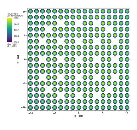
Figure 6a shows the temperature distribution in the solid at z=100 cm at the final Picard iteration
10EPJ Web of Conferences 247, 06053 (2021) https://doi.org/10.1051/epjconf/202124706053
PHYSOR2020
as calculated by Nek5000. The peak fuel centerline temperature at this axial level is 1050 K. We
see that the shape of the distribution roughly matches the heat generation rate, with higher temper-
atures near the guide tubes and lower temperatures away from them in the corners of the assembly.
Figure 6b shows the temperature distribution in the fluid near the outlet on the final Picard iteration
as calculated by Nek5000. The shape of the temperature distribution at the outlet closely matches
the shape of the heat generation shown in Fig. 5. The outlet has an average temperature of about
588 K. With an inlet temperature of 531.5 K, this means the temperature rise across the length of
the assembly is 56.5 K or 101◦ F, agreeing with the NuScale design specification [17] that lists a
ΔT of 100◦ F.
(a) Solid at z=100 cm (b) Fluid at z=200 cm
Figure 6: Temperature distribution as calculated by Nek5000.
To give an idea of the resource requirements to reached a converged solution, which based on
Fig. 4b requires four Picard iterations, we note that the coupled OpenMC-Nek5000 simulation took
three hours to complete four iterations running on 512 nodes of the ALCF Theta supercomputer.
This translates to about 1500 node-hours or 100,000 core-hours.
We note that the same full-length assembly problem run with Shift/Nek5000 produced nearly iden-
tical results. Shift computed a keff at convergence of 1.16673 compared with 1.16693 for OpenMC
and a maximum temperature of 1044 K compared with 1051 K for OpenMC/Nek5000. Given that
OpenMC and Shift are developed independently, use nuclear data processed from two different
codes, and do not share the same model geometry files, the level of agreement between the two
codes on this problem is remarkable and gives us a high degree of confidence in the accuracy of
the solution.
11EPJ Web of Conferences 247, 06053 (2021) https://doi.org/10.1051/epjconf/202124706053
PHYSOR2020
4. CONCLUSIONS
An open source coupling driver application, ENRICO, has been developed for performing high-
fidelity coupled neutronic and thermal-hydraulic (primarily MC and CFD) simulations and is avail-
able at https://github.com/enrico-dev/enrico. The application has been designed such that most of
the control flow logic and implementation is agnostic to the actual code used. Currently, ENRICO
is capable of using the Shift and OpenMC Monte Carlo codes, the Nek5000 spectral element CFD
code, and a simplified subchannel/heat diffusion solver. All data transfers are performed in mem-
ory via C/C++ APIs exposed by each physics code. Results of a coupled simulation on an SMR
fuel assembly problem demonstrated the accuracy of the software. Independent solutions using
OpenMC/Nek5000 and Shift/Nek5000 produced nearly identical results.
Future work to further improve the accuracy of the coupled solution and reduce the time to solution
would be worthwhile. In particular, the solution to the energy equation in Nek5000 is currently
found by running a time-dependent solver until it reaches equilibrium. Implementation of a steady-
state solver in Nek5000 could help substantially reduce the time to solution. For a realistic solution,
however, any future work must also account for turbulence and the effect of grid spacers. This will
assuredly increase the number of elements and hence the computational resources required. Other
means of reducing the time to solution will be needed for such calculations to be practical. One
option may be to use the surrogate heat-fluids solver as a means of quickly iterating to an approxi-
mate solution before starting the Nek5000 simulation. Utilization of newer computer architectures
such as GPUs may help improve the performance per node and reduce the overall time to solution.
However, GPUs will also introduce complexities in how MPI communicators are set up and data
transfers are performed.
ACKNOWLEDGMENTS
This research was supported by the Exascale Computing Project (ECP), Project Number: 17-SC-
20-SC, a collaborative effort of two DOE organizations—the Office of Science and the National
Nuclear Security Administration—responsible for the planning and preparation of a capable ex-
ascale ecosystem—including software, applications, hardware, advanced system engineering, and
early testbed platforms—to support the nation’s exascale computing imperative. This research
used resources of the Argonne Leadership Computing Facility, which is a DOE Office of Science
User Facility supported under contract DE-AC02-06CH11357. This research also used resources
of the Oak Ridge Leadership Computing Facility, which is a DOE Office of Science User Facility
supported under Contract DE-AC05-00OR22725.
REFERENCES
[1] V. Seker, J. W. Thomas, and T. J. Downar. “Reactor simulation with coupled Monte Carlo
and computational fluid dynamics.” In Joint International Topical Meeting on Mathematics
& Computation and Supercomputing in Nuclear Applications. Monterey, California (2007).
[2] J. N. Cardoni and Rizwan-uddin. “Nuclear reactor multi-physics simulations with coupled
MCNP5 and STAR-CCM+.” In Int. Conf. on Mathematics and Computational Methods Ap-
plied to Nuclear Science and Engineering. Rio de Janeiro, Brazil (2011).
[3] J. Hu and Rizwan-Uddin. “Coupled Neutronic and Thermal-Hydraulics Simulations Using
MCNP and FLUENT.” Trans. Am. Nucl. Soc., volume 98(1), pp. 606–608 (2008).
12EPJ Web of Conferences 247, 06053 (2021) https://doi.org/10.1051/epjconf/202124706053
PHYSOR2020
[4] Y. Qiu, P. Lu, U. Fischer, P. Pereslavtsev, and S. Kecskes. “A generic data translation scheme
for the coupling of high-fidelity fusion neutronics and CFD calculations.” Fusion Eng. Des.,
volume 89, pp. 1330–1335 (2014).
[5] X. Wang, D. Zhang, M. Wang, W. Tian, S. Qiu, and G. Su. “A Mesh Mapping Method
for MCNP and FLUENT Coupling Simulation.” Trans. Am. Nucl. Soc., volume 117(1), pp.
739–741 (2017).
[6] H. Breitkreutz, A. Röhrmoser, and W. Petry. “3-Dimensional Coupled Neutronic and
Thermal-Hydraulic Calculations for a Compact Core Combining MCNPX and CFX.” IEEE.
Trans. Nucl. Sci., volume 57(6), pp. 3667–3671 (2010).
[7] X. Xi, Z. Xiao, X. Yan, Y. Li, and Y. Huang. “The axial power distribution validation of
the SCWR fuel assembly with coupled neutronic-thermal hydraulics method.” Nucl. Eng.
Design, volume 258, pp. 157–163 (2013).
[8] L.-S. Li, H.-M. Yuan, and K. Wang. “Coupling of RMC and CFX for analysis of Pebble Bed-
Advanced High Temperature Reactor core.” Nucl. Eng. Design, volume 250, pp. 385–391
(2012).
[9] A. Schulze, H.-J. Allelein, and S. Kelm. “Towards a coupled simulation of thermal hydraulics
and neutronics in a simplified PWR with a 3x3 pin assembly.” In Int. Topical Meeting on
Nuclear Reactor Thermal Hydraulics. Chicago, Illinois (2016).
[10] R. Henry, I. Tiselj, and L. Snoj. “Transient CFD/Monte-Carlo neutron transport coupling
scheme for simulation of a control rod extraction in TRIGA reactor.” Nucl. Eng. Design,
volume 331, pp. 302–312 (2018).
[11] K. E. Remley, D. P. Griesheimer, K. J. Hogan, and J. John R. Buchanan. “Investigations into
coupling the MC21 Monte Carlo transport code to the CFX computational fluid dynamics
code.” In Int. Conf. Mathematics & Computational Methods Applied to Nuclear Science &
Engineering. Portland, Oregon (2019).
[12] R. Tuominen, V. Valtavirta, J. Peltola, and J. Leppänen. “Coupling Serpent and OpenFOAM
for neutronics - CFD multi-physics calculations.” In PHYSOR. Sun Valley, Idaho (2016).
[13] A. Novak, P. Romano, B. Wendt, R. Rahaman, E. Merzari, L. Kerby, C. Permann, R. Mar-
tineau, and R. N. Slaybaugh. “Preliminary coupling of OpenMC and Nek5000 within the
MOOSE framework.” In PHYSOR. Cancun, Mexico (2018).
[14] S. P. Hamilton and T. M. Evans. “Continuous-energy Monte Carlo neutron transport on GPUs
in the Shift code.” Ann. Nucl. Energy, volume 128, pp. 236–247 (2019).
[15] Y. Qiu, L. Lu, and U. Fischer. “A Fusion-Oriented Neutronics Modeling and Multiphysics
Coupling System.” Nucl. Sci. Eng., volume 185, pp. 130–138 (2017).
[16] NuScale Power, LLC. “NuFuel-HTP2TM Fuel and Control Rod Assembly Designs.” Tech-
nical Report TR-0816-51127-NP Rev. 1, NuScale Power (2017). URL https://www.nrc.gov/
docs/ML1700/ML17007A001.pdf.
[17] NuScale Power, LLC. “NuScale Standard Plant Design Certification Application; Chapter
Four: Reactor.” Technical Report ML18310A325, US NRC (2018).
[18] J. Liang, X. Peng, S. Liu, C. Josey, B. Forget, and K. Smith. “Processing of a comprehensive
windowed multipole library via vector fitting.” In PHYSOR. Cancun, Mexico (2018).
13You can also read