Effect of repetition on the behavioral and neuronal responses to ambiguous Necker cube images - Nature
←
→
Page content transcription
If your browser does not render page correctly, please read the page content below
www.nature.com/scientificreports
OPEN Effect of repetition
on the behavioral and neuronal
responses to ambiguous Necker
cube images
Vladimir Maksimenko1,2*, Alexander Kuc1, Nikita Frolov1, Semen Kurkin1 &
Alexander Hramov1,2
A repeated presentation of an item facilitates its subsequent detection or identification, a
phenomenon of priming. Priming may involve different types of memory and attention and affects
neural activity in various brain regions. Here we instructed participants to report on the orientation
of repeatedly presented Necker cubes with high (HA) and low (LA) ambiguity. Manipulating the
contrast of internal edges, we varied the ambiguity and orientation of the cube. We tested how both
the repeated orientation (referred to as a stimulus factor) and the repeated ambiguity (referred to
as a top-down factor) modulated neuronal and behavioral response. On the behavioral level, we
observed higher speed and correctness of the response to the HA stimulus following the HA stimulus
and a faster response to the right-oriented LA stimulus following the right-oriented stimulus. On
the neuronal level, the prestimulus theta-band power grew for the repeated HA stimulus, indicating
activation of the neural networks related to attention and uncertainty processing. The repeated
HA stimulus enhanced hippocampal activation after stimulus onset. The right-oriented LA stimulus
following the right-oriented stimulus enhanced activity in the precuneus and the left frontal gyri
before the behavioral response. During the repeated HA stimulus processing, enhanced hippocampal
activation may evidence retrieving information to disambiguate the stimulus and define its
orientation. Increased activation of the precuneus and the left prefrontal cortex before responding to
the right-oriented LA stimulus following the right-oriented stimulus may indicate a match between
their orientations. Finally, we observed increased hippocampal activation after responding to the
stimuli, reflecting the encoding stimulus features in memory. In line with the large body of works
relating the hippocampal activity with episodic memory, we suppose that this type of memory may
subserve the priming effect during the repeated presentation of ambiguous images.
Perception and memory are the essential brain functions that help us interact with each other and the environ-
ment. Perception reflects the identification and interpretation of sensory evidence to understand the presented
information. Memory stands for the faculty by which the brain encodes sensory or other information, stores,
and retrieves it when needed. Memory influences our perceptual abilities so that we recognize better the objects
we have seen before1. A growing body of literature examines this effect in experimental paradigms, including the
repeatedly presented sensory stimuli. They provide substantial experimental evidence that repeated presentation
of an item facilitates its subsequent detection or identification, a phenomenon known as priming2. This effect
also persists when reexperiencing particular features, such as color or shape, but not the stimulus as a whole.
For instance, in a visual search task, if the target color on the present trial is red, as it was on the previous trial,
a search is facilitated, whereas the green target color slows the s earch1.
riming3. There is a view that feature-based
Literature refers to these effects as object-based and feature-based p
priming engages an implicit memory, whereas object-based priming relies on the explicit m emory4. Implicit
memory allows people to perform specific tasks without conscious awareness of these previous experiences.
In contrast, explicit memory refers to the conscious, intentional recollection of previous experiences and con-
cepts. Probably, these types of priming also relate to the bottom-up and top-down components of attention. The
1
Neuroscience and Cognitive Technology Laboratory, Center for Technologies in Robotics and Mechatronics
Component, Innopolis University, 1 Universitetskaya str., Innopolis, Republic of Tatarstan, Russia 420500. 2Saratov
State Medical University, 112 Bolshaya Kazachia str., Saratov, Russia 410012. *email: maximenkovl@gmail.com
Scientific Reports | (2021) 11:3454 | https://doi.org/10.1038/s41598-021-82688-1 1
Vol.:(0123456789)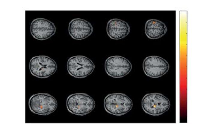
www.nature.com/scientificreports/
bottom-up component refers to involuntary attentional guidance to salient stimuli because of their inherent
properties relative to the background. The top-down component refers to the internal guidance of attention
based on prior knowledge and current goals5. According to Kristjansson et al., the stimuli and the circumstances
of the task in each case dictate what sort of priming occurs3.
Thus, priming occurs at many different levels of the perceptual hierarchy ranging from lower (feature-based)
to higher (object-based) levels, depending on the stimulus, task, and context. Therefore, it appears to modulate
neuronal activity in different brain regions. Neuroimaging studies reported a deceased fMRI signal for primed
vs. unprimed stimuli in various brain regions, a phenomenon called repetition suppression. The repetition sup-
pression in posterior regions evidenced priming of perceptual processes. The effect in more anterior (prefrontal)
regions accompanied priming of conceptual p rocesses6. In addition to repetition suppression, repeated stimulus
presentation can also enhance brain responses relative to its first presentation, a phenomenon called repetition
enhancement. While the repetition enhancement usually occurs in the brain regions associated with explicit mem-
ory, reflecting incidental conscious memory for the previous encounter with a stimulus, it has occasionally been
reported in the brain regions associated with priming, showing repetition suppression under other c onditions7.
Here we analyzed how repetition affected the behavioral and neuronal responses to ambiguous visual stimuli,
Necker cubes. We instructed subjects to respond to the cube’s orientation (left or right). Manipulating the con-
trast of internal edges, we varied the ambiguity and orientation of the cube. We assumed that the brain treated
the contrast of separate edges on the low processing levels and defined the orientation at the higher levels. The
Necker cubes with low (LA) and high (HA) ambiguity had almost the same morphology, and we assumed their
similar processing on low l evels8. We also supposed that responding to HA stimulus orientation required more
information; therefore, HA processing lasted longer, causing greater neuronal response on higher levels. Finally,
we hypothesized that high ambiguity made the subjects to rely on the top-down processes, such as expectations
and memory9. Thus, we tested how both the repeated orientation (stimulus factor) and the repeated ambiguity
(top-down factor) modulated neuronal and behavioral response.
On the behavioral level, we observed higher speed and correctness of the response to the HA stimulus follow-
ing the HA stimulus and a faster response to the right-oriented LA stimulus following the right-oriented stimulus.
The prestimulus theta-band power grew when the HA stimulus followed the HA stimulus. The source analy-
sis revealed an increased activation of the right and the left insula, right frontal cortex, and the left postcentral
cortex. It may indicate activation of the neural networks related to attention and uncertainty processing before
HA stimulus onset. The repeated HA stimulus enhanced activity in the thalamus, hippocampus, and the left
parietal and postcentral gyri for 0.1–0.35 s post-stimulus onset. The right-oriented LA stimulus following the
right-oriented stimulus enhanced activity in the precuneus and the left inferior frontal gyri for ∼ 0.3 s before
the behavioral response. Together, these results may suggest that stimulus processing relies on the matching
information between the current and previously presented stimuli. Increased hippocampal activation during the
earlier (0.1–0.3 s) stage of HA stimulus processing may evidence retrieving information to disambiguate it and
define the orientation. Increased activation of the precuneus and the left prefrontal cortex before responding to
the right-oriented LA stimulus following the right-oriented stimulus may indicate a match between the orienta-
tions at the higher processing levels. Finally, we observed an increased hippocampal activation for ∼ 1.5 s after
responding to the HA stimuli and the right-oriented stimuli. It may reflect the encoding of the percept-related
and the decision-related stimulus features in memory after its offset.
Our finding coincides with a very recent work of Kim et al.10 manifesting that neural repetition suppression
of neuron-level activity in the hippocampus accompanies enhanced EEG power at low frequencies. In line with
the large body of works relating the hippocampal activity with episodic memory, we suppose that this type of
memory may subserve the priming effect during the repeated presentation of ambiguous images.
Methods
Participants. Twenty healthy subjects (9 females) aged 26–35 with normal or corrected-to-normal visual
acuity participated in the experiments. All of them provided written informed consent in advance. All par-
ticipants were familiar with the experimental task and did not participate in similar experiments in the last six
months. The experimental studies were performed under the Declaration of Helsinki and approved by the local
Research Ethics Committee of the Innopolis University.
Experimental procedure. We chose an ambiguous drawing of a Necker cube as a bistable visual stimu-
lus 11–13. The ambiguity, as well as the orientation of the cube’s image, was determined by the balance between
the brightness of the inner edges forming a left-lower (bl = 1 − a) and right-upper (br = a) squares, where
a ∈ [0, 1] was a normalized edge’s luminance in a gray-scale palette. Thus, the limit cases of a = 0 and a = 1
corresponded to unambiguous 2D projections of left- and right-oriented cubes, respectively, whereas a = 0.5
determined a completely ambiguous cube’s image.
In our experiment, we used a set of the Necker cube images with a = {0.15, 0.25, 0.4, 0.45, 0.55, 0.6, 0.75, 0.85}
(Fig. 1A). On the one hand, this set could be separated into subsets of left-oriented a = {0.15, 0.25, 0.4, 0.45}
and right-oriented cubes a = {0.55, 0.6, 0.75, 0.85}. On the other hand, in accordance with our previous s tudy14,
this set could be also divided into low-ambiguous (LA) images a = {0.15, 0.25, 0.75, 0.85}, which are easily
interpreted by an observer, and high-ambiguous (HA) images a = {0.40, 0.45, 0.55, 0.60}, whose interpretations
requires more effort.
We demonstrated 14.2 cm Necker cubes on a white background using a 24′ ′ monitor with the 1920 × 1080
pixels resolution and 60 Hz refresh rate. The distance between the subject and the monitor was 0.7–0.8 m, and
a visual angle was ∼ 0.25 rad. The whole experiment lasted around 40 min for each participant, including short
recordings of the eyes-open resting EEG state (≈ 150 s) before and after the main part of the experiment. During
Scientific Reports | (2021) 11:3454 | https://doi.org/10.1038/s41598-021-82688-1 2
Vol:.(1234567890)
www.nature.com/scientificreports/

                                  Figure 1.  The set of visual stimuli includes Necker cubes with different orientation and ambiguity (A). The
                                  experimental procedure (B) contains 400 stimuli presentations alternating with abstract image presentations;
                                  RT defines the subject’s response time. (C) The time intervals of interest, TOI: TOI1—a 2 s interval time-locked
                                  to the current stimulus onset including 1.5 s prestimulus and 0.5 s post-stimulus segments; TOI2—a 0.5 s
                                  interval preceded the behavioral response to the current stimulus; TOI3—a 1.5 s interval followed the behavioral
                                  response to the previously presented stimulus.

                                  experimental sessions, the cubes with predefined values of a (chosen from the set in Fig. 1A) were randomly
                                  demonstrated 400 times, each cube with a particular ambiguity was presented about 50 times.
                                      We randomized parameter a in the following way. First, we formed a vector A(1...400), including all images
                                  (50 images for each value of a). Then, we randomized indexes in this vector by using the function randperm
                                  in MATLAB. It returned a row vector containing a random permutation of the indexes from 1 to 400 without
                                  repeating elements. Finally, this randomized vector of indexes determined the order of stimuli presentation. We
                                  randomized time of the stimuli presentations and pauses between them as tmin + rand ∗ (tmax − tmin ). Here, tmax
                                  and tmin defined minimal and maximal presentation/pause time, and rand is a MATLAB function that returns
                                  a single uniformly distributed random number in the interval (0,1).
                                      Each i-th stimulus exhibition lasted for a time interval of τ and varied from τmin = 1 s to τmax = 1.5 s. Pauses,
                                  γ between the subsequent presentations of the Necker cube images contained the abstract picture exhibition and
                                  varied from γmin = 3 s to γmax = 5 s (Fig. 1B). We instructed participants to press either the left or right key,
                                  responding to the left or the right stimulus orientation. For each stimulus, we estimated a behavioral response
                                  by measuring the response time, RT, which corresponded to the time passed from the stimulus presentation to
                                  button pressing (Fig. 1B).

                                  EEG recording and processing. The EEG signals were recorded using the monopolar registration method
                                  and the classical extended 10–10 electrode scheme. We recorded 31 signals with two reference electrodes A1

Scientific Reports |   (2021) 11:3454 |                https://doi.org/10.1038/s41598-021-82688-1                                                    3

                                                                                                                                                Vol.:(0123456789)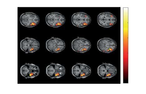
www.nature.com/scientificreports/
and A2 on the earlobes and a ground electrode N just above the forehead. The signals were acquired via the cup
adhesive Ag/AgCl electrodes placed on the “Tien–20” paste (Weaver and Company, Colorado, USA). Imme-
diately before the experiments started, we performed all necessary procedures to increase skin conductivity
and reduce its resistance using the abrasive “NuPrep” gel (Weaver and Company, Colorado, USA). After the
electrodes were installed, the impedance was monitored throughout the experiments. Usually, the impedance
values varied within a 2–5 k interval. The electroencephalograph “Encephalan-EEG-19/26” (Medicom MTD
company, Taganrog, Russian Federation) with multiple EEG channels and a two-button input device (keypad)
was used for amplification and analog-to-digital conversion of the EEG signals. This device possessed the regis-
tration certificate of the Federal Service for Supervision in Health Care No. FCP 2007/00124 of 07.11.2014 and
the European Certificate CE 538571 of the British Standards Institute (BSI). The raw EEG signals were filtered by
a band-pass FIR filter with cut-off points at 1 Hz (HP) and 100 Hz (LP) and by a 50-Hz notch filter by embedded
a hardware-software data acquisition complex. Eyes blinking and heartbeat artifact removal was performed by
Independent Component Analysis (ICA) using EEGLAB software15.
We divided preprocessed EEG signals into trials. We considered two trials for each stimulus: the first trial had
a length of 4 s, and its middle point was time-locked to the stimulus presentation. The second one also had a 4 s
length, but its middle point was time-locked to the behavioral response (when the subject pressed the button).
We calculated wavelet power (WP) in the frequency band of 4–40 Hz using the Morlet wavelet for each trial.
The number of cycles, n depended on the signal frequency, f, as n = f . To minimize between-subject variability,
we considered normalized wavelet power (NWP) by contrasting WP on all trials to the WP averaged over 40-s
baseline EEG before the experiment: NWP = (WP − WPbaseline )/WPbaseline . All calculations were performed
using the Fieldtrip toolbox in MATLAB. After the EEG preprocessing procedure, we excluded some trials due
to the remaining high-amplitude artifacts. As a result, the number of trials varied from 170 to 296 (M=227,
SD=42) in a group of subjects.
Unlike the other works on ambiguous stimuli p rocessing16,17, we did not present completely ambiguous
stimuli, such as a fully symmetrical cube with a = 0.5. Moreover, we instructed subjects to be as correct as pos-
sible. Therefore, we supposed that the subjects responded on the cube orientation based on the acquired sensory
information, rather than the internal r epresentations9. The subjects’ overall correctness rates (CR) varied from
75.5 to 100% (M = 95.1%, SD = 6.4%). Based on the correction rate, we excluded two subjects with CR of 75.5%
and 80.0% as they exceeded the 90th percentile of CR distribution in the group. As a result, we proceeded with
18 subjects (M = 97.07%, SD = 2.6%). In this work, we focused on the effect of the previous stimulus. To ensure
that the subject accurately processed the previous stimulus, we excluded all trials with erroneous responses to
previous stimuli. The amount of excluded trials varied from 1.4 to 18.9% (M = 9.8%, SD = 4.2%) of the initial
number of trials.
Statistical analysis. We performed the group-level statistics for the median RT and the CR for the current
cube depending on the four different factors: current ambiguity, current orientation, previous ambiguity, previ-
ous orientation. We also contrasted the median presentation time (PT) across the same conditions to control the
possible bias of presentation time. The main effects were evaluated via repeated-measures ANOVA. The post hoc
analysis used either paired samples t-test or Wilcoxon signed-rank test, depending on the samples’ normality.
Normality was tested via the Shapiro-Wilk test. We performed a statistical analysis using SPSS.
We analyzed NWP in the frequency band of 1–40 Hz in the three time-intervals of interest (TOI) (Fig. 1C).
The first TOI was a 2 s interval time-locked to the current stimulus onset and included 1.5 s prestimulus and
0.5 s post-stimulus segments. The second TOI reflected a 0.5 s interval preceded the behavioral response to the
current stimulus. Finally, the third TOI reflected a 1.5 s period followed the behavioral response to the previ-
ously presented stimulus.
To contrast the sensor-level NWP we used paired t-test in conjunction with the nonparametric cluster-based
correction for the multiple comparisons and the Monte-Carlo randomization. Cluster formation required at least
two neighboring sensors. A cluster was significant when the p value was below 0.05, corresponding to a false
alarm rate of 0.05 in a two-tailed test. The number of permutations was 1000.
The source power was also contrasted via a paired t-test with the nonparametric cluster-based correction for
the multiple comparisons. A cluster was significant when the p value was below 0.05, corresponding to a false
alarm rate of 0.05 in a two-tailed test. The number of permutations was 2000. We performed sensor-level and
source-level statistical analysis in the Fieldtrip toolbox for MATLAB.
Source localization. We analyzed the source power in the predefined time-frequency domain chosen
based on the sensor-level analysis. Using the exact low-resolution brain electromagnetic tomography (eLO-
RETA) method, we solved the inverse problem and reconstructed source activity from the EEG at each of
the predefined points over brain v olume18–20. “Colin27” brain MRI averaged template21 was used to develop a
boundary element method (BEM) head model with three layers (brain, skull, and scalp)22,23 and source space
consisting of 11865 voxels inside the brain. We fitted the EEG electrodes’ positions to the template head shape.
First, we re-referenced EEG signals to the common average, demeaned them, and filtered by the fourth-order
Butterworth bandpass filter with the passband fL and fH representing the frequencies of interest. Then, we per-
formed time-lock averaging across the trials in each condition and computed the covariance matrix. Finally, we
normalized the resulted source power P in each condition to the 40-s baseline EEG recorded at the beginning of
the experiment as (P − Pbaseline )/Pbaseline . To match the sources’ locations with the brain’s anatomical regions, we
used the Automated Anatomical Labeling (AAL) brain a tlas24. All operations were performed using the Fieldtrip
toolbox in MATLAB25.
Scientific Reports | (2021) 11:3454 | https://doi.org/10.1038/s41598-021-82688-1 4
Vol:.(1234567890)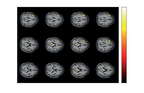
www.nature.com/scientificreports/

                                   Factors                                                                               dF1   dF2   F          p
                                   Current ambiguity                                                                     1     17    61.701     < .001***
                                   Current orientation                                                                   1     17     2.527         .130
                                   Previous ambiguity                                                                    1     17     1.751         .203
                                   Previous orientation                                                                  1     17        .402       .535
                                   Current ambiguity * Current orientation                                               1     17     4.993         .039*
                                   Current ambiguity * Previous ambiguity                                                1     17     6.408         .022*
                                   Current orientation * Previous ambiguity                                              1     17     1.140         .301
                                   Current ambiguity * Current orientation * Previous ambiguity                          1     17        .338       .569
                                   Current ambiguity * Previous orientation                                              1     17     1.549         .230
                                   Current orientation * Previous orientation                                            1     17        .034       .856
                                   Current ambiguity * Current orientation * Previous orientation                        1     17     7.853         .012*
                                   Previous ambiguity * Previous orientation                                             1     17        .750       .399
                                   Current ambiguity * Previous ambiguity * Previous orientation                         1     17        .525       .478
                                   Current orientation * Previous ambiguity * Previous orientation                       1     17        .089       .769
                                   Current ambiguity * Current orientation * Previous ambiguity * Previous orientation   1     17     2.002         .175

                                  Table 1.  Median Response time to the current stimulus, RT [s] (ANOVA Summary).

                                  Figure 2.  Effect of the current stimulus orientation and ambiguity on the RT, regardless of the previous
                                  stimulus orientation and ambiguity. Box-plot illustrates the median RT in the group of subjects for (A) HA and
                                  LA stimuli, p < .001∗∗∗. (B) HA stimuli with left and right orientations, p = .3. (C) LA stimuli with left and
                                  right orientation, p < .01∗∗.

                                  Results
                                  Results of behavioral response analysis. We found a significant main effect of the current stimulus ambiguity
                                  on the RT (Table 1). It indicated that all subjects responded to the LA stimuli (M= .84 s, SD= .26) faster than to
                                  the HA stimuli (M= 1.07 s, SD= .26): t(17) = −8.125, p < .001 (Fig. 2A). There was a main effect of the current
                                  ambiguity on the CR (Table 2). We observed that the CR for the LA stimuli was higher than for the HA stimuli.
                                  According to the Table 3, the presentation times of the HA and LA stimuli did not differ.
                                      A significant interaction effect of the current stimulus ambiguity and orientation on the RT (Table 1) sug-
                                  gested that the RT might differ between the left- and right-oriented stimuli depending on their ambiguity. The
                                  post-hoc analysis demonstrated that the RT remains similar for the left-oriented (M= 1.1 s, SD= .27) and the
                                  right-oriented (M= 1.07 s, SD= .27) HA stimuli: t(17) = 1.07, p = .3 (Fig. 2B). In contrast, 16 subjects responded
                                  faster to the left-oriented LA stimuli (M= .82 s, SD= .26) than to the right-oriented ones (M= .88 s, SD= .29):
                                  Z = −3.114, p = .002 (Fig. 2C). The main effects of the current ambiguity and current orientation on both the
                                  CR (Table 2) and the PT (Table 3) were insignificant.
                                      Regarding the previous stimulus influence, we reported a significant interaction effect of the current and the
                                  previous stimuli ambiguity on RT (Table 1). We could interpret this interaction as the meaning that the previous
                                  stimulus ambiguity affected the RT to the current stimulus differently depending on its ambiguity. The post-
                                  hoc analysis revealed that 15 subjects responded faster to the HA stimuli if the previous stimulus was also HA
                                  (M= 1.05 s, SD= .26) than for the previous LA stimuli (M= 1.1 s, SD= .26): t(17) = −2.64, p = .017 (Fig. 3A).
                                  On the contrary, RT to the LA stimulus after the HA stimulus (M= .85 s, SD= .27) was similar as after the LA
                                  one (M= .84 s, SD= .27): Z = −.348, p = .727 (Fig. 3B). Besides, there was a significant interaction effect of the

Scientific Reports |   (2021) 11:3454 |                     https://doi.org/10.1038/s41598-021-82688-1                                                           5

                                                                                                                                                            Vol.:(0123456789)
www.nature.com/scientificreports/
Factors dF1 dF2 F p
Current ambiguity 1 17 12.379 .003**
Current orientation 1 17 .618 .443
Previous ambiguity 1 17 1.788 .199
Previous orientation 1 17 .386 .543
Current ambiguity * Current orientation 1 17 1.455 .244
Current ambiguity * Previous ambiguity 1 17 6.682 .019*
Current orientation * Previous ambiguity 1 17 4.491 .049*
Current ambiguity * Current orientation * Previous ambiguity 1 17 2.723 .117
Current ambiguity * Previous orientation 1 17 .718 .409
Current orientation * Previous orientation 1 17 2.992 .102
Current ambiguity * Current orientation * Previous orientation 1 17 2.992 .399
Previous ambiguity * Previous orientation 1 17 .076 .786
Current ambiguity * Previous ambiguity * Previous orientation 1 17 .105 .750
Current orientation * Previous ambiguity * Previous orientation 1 17 2.608 .125
Current ambiguity * Current orientation * Previous ambiguity * Previous orientation 1 17 4.111 .059
Table 2. Percentage of correct responses on the current stimulus, CR [%] (ANOVA Summary).
Factors dF1 dF2 F p
Current ambiguity 1 17 2.1 .165
Current orientation 1 17 1.7 .21
Previous ambiguity 1 17 1.079 .313
Previous orientation 1 17 .474 .5
Current ambiguity * Current orientation 1 17 .868 .364
Current ambiguity * Previous ambiguity 1 17 .507 .486
Current orientation * Previous ambiguity 1 17 .037 .849
Current ambiguity * Current orientation * Previous ambiguity 1 17 .037 .468
Current ambiguity * Previous orientation 1 17 .1 .921
Current orientation * Previous orientation 1 17 .443 .515
Current ambiguity * Current orientation * Previous orientation 1 17 3.222 .09
Previous ambiguity * Previous orientation 1 17 .215 .649
Current ambiguity * Previous ambiguity * Previous orientation 1 17 1.63 .219
Current orientation * Previous ambiguity * Previous orientation 1 17 .154 .7
Current ambiguity * Current orientation * Previous ambiguity * Previous orientation 1 17 4.111 0.002**
Table 3. Median presentation time of the current stimulus, PT [c] (ANOVA Summary).
current ambiguity and the previous ambiguity on the CR (Table 2). At the same time, it failed to achieve signifi-
cance in the post-hoc tests. Finally, the interaction effect of the current ambiguity and the previous ambiguity
on the PT was insignificant (Table 3). Since the effect of the previous stimulus was central in this manuscript,
we additionally considered the PT distributions of the HA stimuli followed the HA and LA stimuli (Fig. 3C)
and contrasted the median PT in these conditions (Fig. 3D). We found that PT varied from 300 s to 2700 s. The
median PT of HA stimuli following HA stimuli (M= 1365 s, SD= 157) did not differ from the median PT of HA
stimuli following LA stimuli (M= 1395 s, SD= 74): t(17) = −.975, p = .355 (Fig. 3D). According to the Fig. 3D,
the differences between some PTs pairs in HA vs. LA conditions are extremely large. To make the RT analysis
in these conditions more convincing, we applied a strict criterion to the PT difference. Setting the threshold
for the absolute PT difference ( PT) as 2.5 × 10² s, we excluded one subject with PT = 3.19 × 10² s from the
consideration. The RT difference in the rest of the subjects remained significant: t(17) = 2.56, p = .021.
Finally, there was a significant interaction effect of the current ambiguity, current orientation, and the previ-
ous orientation on the RT (Table 1). Within the post-hoc analysis, we considered RT separately for HA and LA
current stimuli via a repeated-measures ANOVA with the current and previous orientation taken as within-
subject factors. For the HA stimuli, neither current nor previous orientations had a significant effect on the
RT (Fig. 4A). For the LA stimuli, there was a significant interaction effect of the previous and current orienta-
tion on the RT: F(1, 17) = 7.262, p = .015. The post-hoc analysis revealed that the RT did not depend on the
previous stimulus orientation for the left-oriented LA stimuli. In contrast, 16 subjects responded faster to the
right-oriented LA stimuli if the previous stimulus was also right-oriented (M= .87 s, SD= .29 ) rather than
after the left-oriented previous stimulus (M= .92 s, SD= .29): Z = −2.809, p = .005 (Fig. 4B). To exclude the
possible effect of the PT bias between the conditions, we considered the PT distributions of the right-oriented
Scientific Reports | (2021) 11:3454 | https://doi.org/10.1038/s41598-021-82688-1 6
Vol:.(1234567890)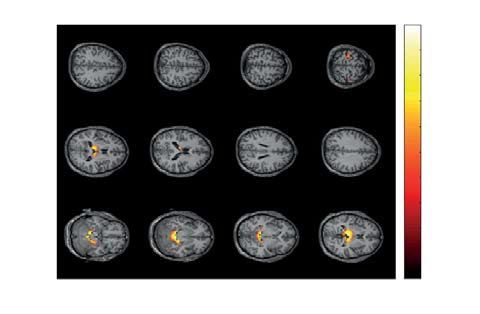
www.nature.com/scientificreports/
Figure 3. Effect of the previous stimulus ambiguity on the RT to the current stimulus. Box-plot illustrates
the median RT in the group of subjects to (A) the HA stimuli, p < .017∗ and (B) LA stimuli, p = .727 (B)
depending on the ambiguity of the previous stimulus. Dot-plot and histograms (C) show PT distributions
for the HA stimuli following the HA and LA stimulus. Box-plot (D) reflects the median PT of the HA stimuli
following the HA and LA stimuli in the group of subjects, p = .355.
Figure 4. Effect of the previous stimulus orientation on RT to the current stimulus. Box-plot (A) illustrates
median RT in the group of subjects to the left-oriented (L) and the right-oriented (R) HA stimuli depending on
the orientation of the previous stimulus ( p > 0.05, ANOVA). Box-plot (B) illustrates median RT for the left-
oriented and the right-oriented LA stimuli depending on the previous stimulus’s orientation p = .005∗∗. Dot-
plot and histograms (C) show distributions of the presentation times for the right-oriented LA stimuli preceded
by right-oriented (R-R) and left-oriented (R-L) stimuli. Box-plot (D) reflects the median presentation times of
the right-oriented LA stimuli preceded by the right-oriented and the left-oriented stimuli, p = .337.
LA stimuli followed the left-oriented (R-L) and the right-oriented (R-R) stimuli (Fig. 4C) and contrasted the
median PT in these conditions (Fig. 4D). We found that PT varied from 3 × 10² s to 27 × 102 s. The median
PT of the right-oriented LA stimuli followed the left-oriented stimuli (R-L) (M= 1389 s, SD= 95) did not differ
from the median PT of the right-oriented LA stimuli followed the right-oriented stimuli (R-R) (M= 1356 s,
SD= 95): t(17) = −.988, p = .337 (Fig. 4D). According to the Fig. 4D, the differences between some PTs pairs
in R-R vs. R-L conditions are also large. Setting the threshold for the absolute PT difference ( PT) as 2.5 × 10² s,
Scientific Reports | (2021) 11:3454 | https://doi.org/10.1038/s41598-021-82688-1 7
Vol.:(0123456789)www.nature.com/scientificreports/
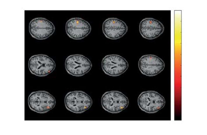
Figure 5. Two significant clusters as the result of NWP comparison during HA stimuli processing following
the HA and LA stimuli on the 2 s interval time-locked to stimulus onset (vertical solid line). The blue and
orange curves (A) show evolution of the NWP (group means and 95% CI) in these clusters during HA stimuli
processing following the LA and HA stimuli. The scalp topogram (B) reflects t-value, and the channels
demonstrating a significant change of NWP between analyzed conditions on the EEG sensor level. The box-plot
(C) illustrates NWP in this cluster averaged over the time interval, frequency band, and channels. The slice-plot
(D) reflects the t-value for the voxels demonstrating a significant change of the source power. pcorr is corrected
for multiple comparisons via the cluster-based test with the Monte-Carlo randomization technique.
we excluded two subjects with PT = 2.63 × 10² s and PT = 2.95 × 10² s from the consideration. The RT
difference in the rest 16 subjects remained significant: t(17) = 2.29, p = .037.
Results of EEG signals analysis. Behavioral analysis indicated that the previous stimulus affected the
current stimulus processing in two cases: i) subjects responded faster to the HA stimuli following the HA stimuli;
ii) subjects responded faster to the right-oriented LA stimuli following the right-oriented stimuli. We analyzed
changes in neural activity that might underly these behavioral effects in three TOI (see Fig. 1C).
First, we contrasted neural activity during processing HA stimuli following HA and LA stimuli. Contrasting
the normalized wavelet power (NWP) on a 2-s interval time-locked to the current stimulus onset, including
1.5-s prestimulus and 0.5-s post-stimulus segments (TOI1 in Fig. 1C), we found two significant positive clusters.
The first sensor-level cluster with p = .042 appeared from .09 s to .37 s post-stimulus onset in the frequency
range of 8 − 8.5 Hz (Fig. 5A, top plot) and included EEG sensors {O2, P4, P8, CP3, CPz, CP4, TP8, C3, Cz, C4,
FT7, FC3, FCz, FC4, FT8} in the right-lateralized occipito-parietal and bilateral central EEG rows (Fig. 5B, top
plot). The averaged NWP in this cluster was higher when the HA stimulus followed the HA stimulus in 14 sub-
jects (Fig. 5C, top plot). For the time-frequency range of this cluster, we calculated source power and contrasted
it between the conditions. As a result, we observed a significant positive cluster with p = .032. This source-level
cluster included the right part of the thalamus, left inferior parietal lobule, left postcentral gyrus, right part of
the hippocampus, and right parahippocampal gyrus (Fig. 5D, top plot). The second sensor-level cluster with
p = .045 appeared from 1.5 s to 1.28 s before stimulus onset in the frequency range of 4 − 5 Hz (Fig. 5A, bottom
plot) and included EEG sensors {P7, P3, Pz, TP7, CP3, CPz, CP4, C3, Cz, C4} mostly in the parietal and central
EEG rows (Fig. 5B, bottom plot). The averaged NWP in this cluster was higher when HA stimulus followed HA
stimulus in 14 subjects (Fig. 5C, bottom plot). We observed a significant positive cluster on the source-level with
p = .022, that included left rolandic operculum, left inferior frontal gyrus, left and right insula, right middle
frontal gyrus, and left postcentral gyrus (Fig. 5D, bottom plot).
Contrasting the NWP on a 0.5 s interval that preceded the behavioral response to the current stimulus (TOI2
in Fig. 1C), we found no significant clusters.
Contrasting the NWP on a 1.5 s period followed the behavioral response to the previously presented stimulus
(TOI3 in Fig. 1C), we found two significant positive clusters on the sensor level. The sensor-level first cluster with
Scientific Reports | (2021) 11:3454 | https://doi.org/10.1038/s41598-021-82688-1 8
Vol:.(1234567890)www.nature.com/scientificreports/
Figure 6. Two significant clusters as the result of NWP comparison after responding to HA and LA stimuli on
the 1.5-s interval time-locked to the behavioral response (vertical solid line). The orange and blue curves (A)
show the NWP evolution (group means and 95% CI) in these clusters after responding to LA and HA stimuli.
The topogram (B) reflects the t-value and the channels demonstrating a significant change of NWP between
analyzed conditions on the EEG sensor level. The box-plot (C) illustrates NWP in this cluster averaged over the
time interval, frequency band, and channels. The slice-plot (D) reflects the t-value for the voxels included in the
source-level cluster. pcorr is corrected for multiple comparisons via the cluster-based test with the Monte-Carlo
randomization technique.
p = .004 appeared from 1.0 to 1.33 s after the behavioral response in the frequency-range of 11–12.5 Hz (Fig. 6A,
top plot). It included EEG sensors {Fz, Fp2, F4, F8, FC4, FT8} in the right-lateralized frontal EEG rows (Fig. 6B,
top plot). The averaged NWP in this cluster was higher after responding to the HA stimulus in all subjects
(Fig. 6C, top plot). We observed a significant positive cluster ( p = .03) on the source-level in this time-frequency
range, including the bilateral frontal gyri, right temporal gyri, right insula, fusiform gyrus, and caudate nucleus
(Fig. 6D, top plot). The second sensor-level cluster with p = .012 appeared from 1.0 to 1.1 s after the behavioral
response in the frequency range of 11.5–12.5 Hz (Fig. 6A, bottom plot). It included EEG sensors {P8, CP4, TP8}
in the right-lateralized temporal EEG rows (Fig. 6B, bottom plot). The averaged NWP in this cluster was higher
after processing HA stimulus in 16 subjects (Fig. 6C, bottom plot). On the source level, it corresponded to a
positive cluster with p = .047, including the left parts of the thalamus, hippocampus, and the parahippocampal
gyrus, as well as the right superior temporal gyrus, and right caudate nucleus (Fig. 6D, bottom plot).
Second, we contrasted neural activity during the right-oriented LA stimulus processing, following the right-
and left-oriented stimuli. Contrasting the NWP on TOI1 we found no significant clusters.
Contrasting the NWP on TOI2, we found one significant positive cluster with p = .048. This sensor-level clus-
ter appeared from .49 to .37 s before the behavioral response in the frequency range of 10.25–10.5 Hz (Fig. 7A).
It included EEG sensors {C3, FT7, FC3} in the left-lateralized central, temporal and frontal EEG rows (Fig. 7B).
The averaged NWP in this cluster was higher when the right-oriented LA stimulus followed the right-oriented
stimuli in 16 subjects (Fig. 7C). For the time-frequency range of this cluster, we calculated source power and
contrasted it between the conditions. Setting the ppairwise = .001, we did not found the source-level clusters. For
the ppairwise = .01 we obtained a positive cluster with p = .172 (Fig. 7D). This source-level cluster included the left
inferior frontal gyrus, left calcarine sulcus, and the left precuneus. These source-level results showed potentially
interesting tendencies without being supported by the cluster-level statistics. To quantify the change of source
power in these zones, we computed Cohen’s d and counted the number of subjects demonstrating the effect. As
a result, we found a medium effect for the left inferior frontal gyrus (d = 0.55, 14 subjects), the left precuneus
(d = 0.49, 15 subjects) and the left calcarine sulcus (d = 0.52, 15 subjects).
Contrasting NWP on TOI3, we found one significant positive cluster with p = .034 in the frequency range
of 11.5–14.5 Hz on the time interval of 1.3–1.5 s after the behavioral response (Fig. 8A). It included EEG sen-
sors {Pz, P4, CPz, CP4, Cz, C4} in the right-lateralized occipito-parietal and central EEG rows (Fig. 8B). The
averaged NWP in this cluster was higher after responding to the right-oriented stimulus in 15 subjects (Fig. 8C).
On the source level, it corresponded to the significant positive cluster with p = .037 , including left and right
Scientific Reports | (2021) 11:3454 | https://doi.org/10.1038/s41598-021-82688-1 9
Vol.:(0123456789)www.nature.com/scientificreports/
Figure 7. Significant cluster as the result of NWP comparison during the right-oriented LA stimuli processing
following the right- and left-oriented stimuli on the 0.5-s interval time-locked to the behavioral response
(vertical solid line). The orange and blue curves (A) show NWP evolution (group means and 95% CI) in this
cluster during the right-oriented LA stimuli processing following the left-oriented and right-oriented stimuli.
The topogram (B) reflects the t-value and the channels demonstrating a significant change of NWP between
analyzed conditions on the EEG sensor level. The box-plot (C) illustrates NWP in this cluster averaged over the
time interval, frequency band, and channels. The slice-plot (D) reflects the t-value for the voxels demonstrating
a significant change of the source power. pcorr is corrected for multiple comparisons via the cluster-based test
with the Monte-Carlo randomization technique.
Figure 8. Significant cluster as the result of NWP comparison after responding to the right- and left-oriented
stimuli on the 1.5-s interval time-locked to the behavioral response (vertical solid line). The orange and blue
curves (A) show the NWP evolution (group means and 95% CI) in these clusters after responding to the left-
and right-oriented stimuli. The topogram (B) reflects the t-value and the channels demonstrating a significant
change of NWP between analyzed conditions on the EEG sensor level. The box-plot (C) illustrates NWP in this
cluster averaged over the time interval, frequency band, and channels. The slice-plot (D) reflects the t-value for
the voxels included in the source-level cluster. pcorr is corrected for multiple comparisons via the cluster-based
test with the Monte-Carlo randomization technique.
parts of the thalamus, hippocampus, parahippocampal gyrus, left precentral and postcentral gyri, cerebellum,
and vermis (Fig. 8D).
Discussion
We revealed that the subjects responded to LA stimuli faster and more correctly than to HA stimuli that coin-
cides with our previous fi ndings12,26. In the latter case, they deal with ambiguous sensory information and may
increasingly rely on the top-down processes, such as expectations and memory, to make a correct d ecision9,13.
When processing LA stimuli, subjects responded quicker to the left-oriented stimuli than to the right-oriented
ones. We suppose that the Necker cube has high spatial dimensions and covers both visual fields. The cube’s
morphology suggested that the sensory evidence for the left orientation appeared mostly in its left part. When
visually examining stimulus from left to right, the observer starts seeing the internal edges that provide addi-
tional information about the right orientation. There is a view that subjects respond faster to the stimuli in the
left visual field due to the right-lateralization of the attentional networks27. Thus, we suppose that participants
Scientific Reports | (2021) 11:3454 | https://doi.org/10.1038/s41598-021-82688-1 10
Vol:.(1234567890)www.nature.com/scientificreports/
quickly find the signs of left-orientation in the left visual field. Future studies should validate this hypothesis by
using eye-tracking systems.
Regarding the previous stimulus effect, we observed higher speed and correctness of the response to HA
stimulus folowing HA stimulus. Moreover, we reported a faster response to the right-oriented LA stimulus fol-
lowing the right-oriented stimulus. We hypothesize that these two behavioral effects result from the different
mechanisms of brain activity. In the first case, we suppose that previous stimulus modulates attentional state
and mobilizes neural networks used for ambiguous stimuli processing. It improves the processing of ongoing
HA stimulus, contributing to its disambiguation and orientation determination. In the second case, we suppose
that the brain learns the signs of the right orientation. It facilitates orientation determination of the ongoing
right-oriented stimulus by matching its orientation with the previously learned one.
Analysis of the prestimulus and post-stimulus neural activity provided evidence supporting our hypothesis.
We observed high prestimulus theta-band power when HA stimulus followed HA stimulus. The source analysis
revealed increased activation of the right and the left insula, right frontal cortex, and the left postcentral cortex.
Activity in the theta-band appears to coordinate neural activity in the remote r egions28, including neural interac-
tions in the fronto-parietal attentional n etworks29. The right insula and right frontal cortex formed the core of
etwork30. Activity in these areas, together with the parietal cortex, increases during visual
a ventral attentional n
tasks. The right insula and right inferior frontal cortex are also among the most critical prefrontal regions for
cognitive control, enabling detecting behaviorally salient s timuli31. Finally, the insular cortex plays a crucial role
in accumulating evidence to process uncertainty in the context of decision-making32. Taken together, it indicates
activation of the neural networks related to attention and uncertainty processing before HA stimulus onset.
Processing of the HA stimulus following the HA stimulus also induced high theta-band power for 0.1–0.35 s
post-stimulus onset. The source analysis revealed increased activation of the thalamus, hippocampus, parahip-
pocampal gyrus, and the left parietal and postcentral gyri. Traditionally, the stimulus-related theta-band power
correlates with memory retrieval and decision making. During retrieval, the power of left-parietal theta oscilla-
tions increased in proportion to how well a test item was r emembered33. Finally, thalamic theta-band power also
increased during r etrieval34. The right-lateralized hippocampal activation is essential to retrieving the sensory-
based memory details35. While the Ref. 35 relates hippocampal activation with the long-term memory, its activity
appears to subserve encoding and retrieval in a working memory p aradigm36,37. These results may suggest that the
processing of HA stimulus utilizes the information retrieved from memory. Increased parahippocampal activity
may also confirm this view. This area exhibits stronger activation when processing old stimulus configurations
than new configurations38.
Improved response time to the right-oriented LA stimulus following the right-oriented stimulus did not
accompany changes of the prestimulus and post-stimulus neural activity. Simultaneously, we observed activation
of the precuneus gyrus and the left inferior frontal gyrus before the behavioral response. Previously, Lundstrom
and colleagues suggested that both the precuneus and the left inferior PFC were essential for the regeneration of
episodic contextual associations and that they activated together during correct source retrieval39,40. The absence
of differences in the post-stimulus period may indicate that retrieval-related increase of power attenuates due
to repetition suppression. Repetition suppression means that the stimulus is the same as a previous event, with
minimal encoding need, and usually reduces the medial temporal lobe activation, including hippocampus41.
Together, these results may suggest that stimulus processing partly relies on the matching information between
the current and previously presented stimuli. Increased hippocampal activation during the earlier (0.1–0.3 s)
stage of HA stimulus processing may evidence retrieving information to disambiguate it and define orientation.
Increased activation of the precuneus and the left prefrontal cortex before responding to the right-oriented LA
stimulus following the right-oriented stimulus may indicate a match between the orientations.
Supposing that the brain retrieves the previous stimulus’s features to process the next stimulus, we inspected
intervals between stimuli to find neural signs of the encoding process. Earlier, Ben-Yakov and Dudai reported
that the hippocampal activation immediately following event offset plays a role in encoding the episode into
memory and can predict subsequent memory for it42. Similarly, we observed increased hippocampal activation
for ∼ 1.5 s after responding to the HA stimuli and the right-oriented LA stimuli. Combining these findings with
the behavioral data, we assume that the interpretation of HA stimulus may require more information than the
interpretation of LA stimulus. Similarly, the interpretation of the right-oriented stimulus requires more infor-
mation than the interpretation of the left-oriented one. After the stimulus offset, the percept-related and the
decision-related stimulus information is encoded in memory. Enhanced hippocampal activation may reflect the
amount of encoded information.
Literature usually associates hippocampal activation and the activation of the precuneus and the left prefron-
tal cortex with the long-term episodic memory and stimulus-stimulus a ssociations43. Simultaneously, the hip-
pocampus subserves the short-term associative m emory44. Associative memory refers to the ability to remember
relationships between two or more items or between an item and its context, e.g., between the pairs of pictures41,43
or between the pictures and w ords45. Grön et al. also reported that hippocampal activation during a response
to the complex geometric patterns might reflect encoding and retrieval of intra-image a ssociations46. Thus,
participants may learn the associations between the Necker cube features in the most demanding cases, such
as HA and the right-oriented LA stimuli. After the offset of these stimuli, these associations are encoded into
the memory. When the previously seen stimulus is reexperienced, the sensory information is matched to stored
memory representations, improving the behavioral response. We suppose that there is a difference between the
HA and the right-oriented LA stimuli. In the first case, the brain encodes stimulus details to use them for defining
the orientation. In the latter case, it learns the signs of the particular (right) orientation. Therefore, we observe
further thalamic activation during HA stimulus processing. The absence of such activation during the right-
oriented LA stimulus processing may reflect that the stimulus orientation matches the previously seen stimulus’s
Scientific Reports | (2021) 11:3454 | https://doi.org/10.1038/s41598-021-82688-1 11
Vol.:(0123456789)www.nature.com/scientificreports/
orientation. Moreover, we suppose that the HA stimulus modulates the attentional network’s activity, including
right-lateralized frontal and temporal cortices, improving the next HA stimulus’s processing.
Finally, this study has limitations. While a high-density EEG enables detecting deep subcortical activity47,
we used a small number of EEG channels, and an averaged MRI, which may not be sufficient for reliable locali-
zation of the reported neuronal activity in source space. Therefore, we did not report the lateralization of the
hippocampal activity, which is also essential for memory encoding and retrieval.
Received: 20 July 2020; Accepted: 20 January 2021
References
1. Kristjánsson, Á. & Campana, G. Where perception meets memory: A review of repetition priming in visual search tasks. Attent.
Percept. Psychophys. 72, 5–18 (2010).
2. Kristjánsson, Á. & Ásgeirsson, Á. G. Attentional priming: Recent insights and current controversies. Curr. Opin. Psychol. 29, 71–75
(2019).
3. Kristjánsson, Á., Ingvarsdöttir, Á. & Teitsdöttir, U. D. Object-and feature-based priming in visual search. Psychon. Bull. Rev. 15,
378–384 (2008).
4. Huang, L., Holcombe, A. O. & Pashler, H. Repetition priming in visual search: Episodic retrieval, not feature priming. Mem. Cognit.
32, 12–20 (2004).
5. Katsuki, F. & Constantinidis, C. Bottom-up and top-down attention: Different processes and overlapping neural systems. Neuro-
scientist 20, 509–521 (2014).
6. Lee, S.-M., Henson, R. & Lin, C.-Y. Neural correlates of repetition priming: A coordinate-based meta-analysis of FMRI studies.
Front. Hum. Neurosci. 14, 379 (2020).
7. Kim, H. Brain regions that show repetition suppression and enhancement: A meta-analysis of 137 neuroimaging experiments.
Hum. Brain Mapp. 38, 1894–1913 (2017).
8. Okazaki, M., Kaneko, Y., Yumoto, M. & Arima, K. Perceptual change in response to a bistable picture increases neuromagnetic
beta-band activities. Neurosci. Res. 61, 319–328 (2008).
9. Engel, A. K. & Fries, P. Beta-band oscillations–signalling the status quo?. Curr. Opin. Neurobiol. 20, 156–165 (2010).
10. Kim, K., Hsieh, L.-T., Parvizi, J. & Ranganath, C. Neural repetition suppression effects in the human hippocampus. Neurobiol.
Learn. Mem. 173, 107269 (2020).
11. Kornmeier, J., Friedel, E., Wittmann, M. & Atmanspacher, H. Eeg correlates of cognitive time scales in the Necker-Zeno model
for bistable perception. Conscious. Cogn. 53, 136–150 (2017).
12. Maksimenko, V. A. et al. Neural interactions in a spatially-distributed cortical network during perceptual decision-making. Front.
Behav. Neurosci. 13, 220 (2019).
13. Maksimenko, V. A. et al. Dissociating cognitive processes during ambiguous information processing in perceptual decision-making.
Front. Behav. Neurosci.14,(2020).
14. Maksimenko, V. A. et al. Increasing human performance by sharing cognitive load using brain-to-brain interface. Front. Neurosci.
12, 949 (2018).
15. Delorme, A. & Makeig, S. Eeglab: An open source toolbox for analysis of single-trial EEG dynamics including independent com-
ponent analysis. J. Neurosci. Methods 134, 9–21 (2004).
16. Kornmeier, J. & Bach, M. Bistable perception–along the processing chain from ambiguous visual input to a stable percept. Int. J.
Psychophysiol. 62, 345–349 (2006).
17. Yokota, Y., Minami, T., Naruse, Y. & Nakauchi, S. Neural processes in pseudo perceptual rivalry: An ERP and time-frequency
approach. Neuroscience 271, 35–44 (2014).
18. Pascual-Marqui, R. D. Discrete, 3d distributed, linear imaging methods of electric neuronal activity. part 1: exact, zero error
localization. arXiv preprint arXiv:0710.3341 (2007).
19. Pascual-Marqui, R. D. et al. Exact low resolution brain electromagnetic tomography (eloreta). Neuroimage 31 (2006).
20. Pascual-Marqui, R. D. Theory of the EEG inverse problem. In Quantitative EEG Analysis: Methods and Clinical Applications121–140
(2009).
21. Holmes, C. J. et al. Enhancement of MR images using registration for signal averaging. J. Comput. Assist. Tomogr. 22, 324–333
(1998).
22. Fuchs, M., Kastner, J., Wagner, M., Hawes, S. & Ebersole, J. S. A standardized boundary element method volume conductor model.
Clin. Neurophysiol. 113, 702–712 (2002).
23. Baillet, S., Mosher, J. C. & Leahy, R. M. Electromagnetic brain mapping. IEEE Signal Process. Mag. 18, 14–30 (2001).
24. Tzourio-Mazoyer, N. et al. Automated anatomical labeling of activations in using a macroscopic anatomical parcellation of the
MNI MRI single-subject brain. Neuroimage 15, 273–289 (2002).
25. Oostenveld, R., Fries, P., Maris, E. & Schoffelen, J.-M. Fieldtrip: Open source software for advanced analysis of MEG, EEG, and
invasive electrophysiological data. Comput. Intell. Neurosci.2011 (2011).
26. Maksimenko, V. A. et al. Visual perception affected by motivation and alertness controlled by a noninvasive brain-computer
interface. PloS ONE12 (2017).
27. Śmigasiewicz, K., Asanowicz, D., Westphal, N. & Verleger, R. Bias for the left visual field in rapid serial visual presentation: Effects
of additional salient cues suggest a critical role of attention. J. Cogn. Neurosci. 27, 266–279 (2014).
28. Berger, B. et al. Dynamic regulation of interregional cortical communication by slow brain oscillations during working memory.
Nat. Commun. 10, 1–11 (2019).
29. Kam, J. W. et al. Default network and frontoparietal control network theta connectivity supports internal attention. Nat. Hum.
Behav. 3, 1263–1270 (2019).
30. Eckert, M. A. et al. At the heart of the ventral attention system: The right anterior insula. Hum. Brain Mapp. 30, 2530–2541 (2009).
31. Cai, W., Chen, T., Ide, J. S., Li, C.-S.R. & Menon, V. Dissociable fronto-operculum-insula control signals for anticipation and
detection of inhibitory sensory cue. Cereb. Cortex 27, 4073–4082 (2017).
32. Singer, T., Critchley, H. D. & Preuschoff, K. A common role of insula in feelings, empathy and uncertainty. Trends Cognit. Sci. 13,
334–340 (2009).
33. Jacobs, J., Hwang, G., Curran, T. & Kahana, M. J. EEG oscillations and recognition memory: Theta correlates of memory retrieval
and decision making. Neuroimage 32, 978–987 (2006).
34. Bauch, E. M. et al. Theta oscillations underlie retrieval success effects in the nucleus accumbens and anterior thalamus: Evidence
from human intracranial recordings. Neurobiol. Learn. Mem. 155, 104–112 (2018).
35. St-Laurent, M., Moscovitch, M. & McAndrews, M. P. The retrieval of perceptual memory details depends on right hippocampal
integrity and activation. Cortex 84, 15–33 (2016).
Scientific Reports | (2021) 11:3454 | https://doi.org/10.1038/s41598-021-82688-1 12
Vol:.(1234567890)www.nature.com/scientificreports/
36. Karlsgodt, K. H., Shirinyan, D., van Erp, T. G., Cohen, M. S. & Cannon, T. D. Hippocampal activations during encoding and
retrieval in a verbal working memory paradigm. Neuroimage 25, 1224–1231 (2005).
37. Öztekin, I., McElree, B., Staresina, B. P. & Davachi, L. Working memory retrieval: Contributions of the left prefrontal cortex, the
left posterior parietal cortex, and the hippocampus. J. Cogn. Neurosci. 21, 581–593 (2009).
38. Düzel, E. et al. Human hippocampal and parahippocampal activity during visual associative recognition memory for spatial and
nonspatial stimulus configurations. J. Neurosci. 23, 9439–9444 (2003).
39. Lundstrom, B. N., Ingvar, M. & Petersson, K. M. The role of precuneus and left inferior frontal cortex during source memory
episodic retrieval. Neuroimage 27, 824–834 (2005).
40. Lundstrom, B. N. et al. Isolating the retrieval of imagined pictures during episodic memory: Activation of the left precuneus and
left prefrontal cortex. Neuroimage 20, 1934–1943 (2003).
41. Zeithamova, D., Manthuruthil, C. & Preston, A. R. Repetition suppression in the medial temporal lobe and midbrain is altered by
event overlap. Hippocampus 26, 1464–1477 (2016).
42. Ben-Yakov, A. & Dudai, Y. Constructing realistic engrams: poststimulus activity of hippocampus and dorsal striatum predicts
subsequent episodic memory. J. Neurosci. 31, 9032–9042 (2011).
43. Öngür, D. et al. Hippocampal activation during processing of previously seen visual stimulus pairs. Psychiatry Res. Neuroimaging
139, 191–198 (2005).
44. Kumaran, D. Short-term memory and the human hippocampus. J. Neurosci. 28, 3837–3838 (2008).
45. Degonda, N. et al. Implicit associative learning engages the hippocampus and interacts with explicit associative learning. Neuron
46, 505–520 (2005).
46. Grön, G. et al. Hippocampal activations during repetitive learning and recall of geometric patterns. Learn. Mem. 8, 336–345 (2001).
47. Seeber, M. et al. Subcortical electrophysiological activity is detectable with high-density EEG source imaging. Nat. Commun. 10,
1–7 (2019).
Acknowledgements
This study is supported by the Russian Science Foundation (19-12-00050) in paradigm development and experi-
ments. NF thanks President Program (NSh-2594.2020.2) for personal support in the sensor-level EEG data
analysis. AK received support from the President Program (MK-1760.2020.2) in the behavioral data analysis,
SK is supported by the President Program (MD-1921.2020.9) in the part of the source reconstruction.
Author contributions
A.H. and V.M. designed the study, V.M. supervised the study, A.K. and N.F. performed the data analysis on the
sensor level, A.K. analyzed behavioral data, S.K. performed the data analysis on the source level, V.M. interpreted
results, prepared illustrations, and wrote the manuscript.
Competing interests
The authors declare no competing interests.
Additional information
Correspondence and requests for materials should be addressed to V.M.
Reprints and permissions information is available at www.nature.com/reprints.
Publisher’s note Springer Nature remains neutral with regard to jurisdictional claims in published maps and
institutional affiliations.
Open Access This article is licensed under a Creative Commons Attribution 4.0 International
License, which permits use, sharing, adaptation, distribution and reproduction in any medium or
format, as long as you give appropriate credit to the original author(s) and the source, provide a link to the
Creative Commons licence, and indicate if changes were made. The images or other third party material in this
article are included in the article’s Creative Commons licence, unless indicated otherwise in a credit line to the
material. If material is not included in the article’s Creative Commons licence and your intended use is not
permitted by statutory regulation or exceeds the permitted use, you will need to obtain permission directly from
the copyright holder. To view a copy of this licence, visit http://creativecommons.org/licenses/by/4.0/.
© The Author(s) 2021
Scientific Reports | (2021) 11:3454 | https://doi.org/10.1038/s41598-021-82688-1 13
Vol.:(0123456789)You can also read