FPGA Design of Enhanced Scale-Invariant Feature Transform with Finite-Area Parallel Feature Matching for Stereo Vision
←
→
Page content transcription
If your browser does not render page correctly, please read the page content below
electronics
Article
FPGA Design of Enhanced Scale-Invariant Feature Transform
with Finite-Area Parallel Feature Matching for Stereo Vision
Chien-Hung Kuo, Erh-Hsu Huang, Chiang-Heng Chien and Chen-Chien Hsu *
Department of Electrical Engineering, National Taiwan Normal University, Taipei 10610, Taiwan;
chk@ntnu.edu.tw (C.-H.K.); 60675013h@ntnu.edu.tw (E.-H.H.); chiangheng.chien@gmail.com (C.-H.C.)
* Correspondence: jhsu@ntnu.edu.tw; Tel.: +886-2-7749-3551
Abstract: In this paper, we propose an FPGA-based enhanced-SIFT with feature matching for stereo
vision. Gaussian blur and difference of Gaussian pyramids are realized in parallel to accelerate the
processing time required for multiple convolutions. As for the feature descriptor, a simple triangular
identification approach with a look-up table is proposed to efficiently determine the direction and
gradient of the feature points. Thus, the dimension of the feature descriptor in this paper is reduced
by half compared to conventional approaches. As far as feature detection is concerned, the condition
for high-contrast detection is simplified by moderately changing a threshold value, which also
benefits the reduction of the resulting hardware in realization. The proposed enhanced-SIFT not only
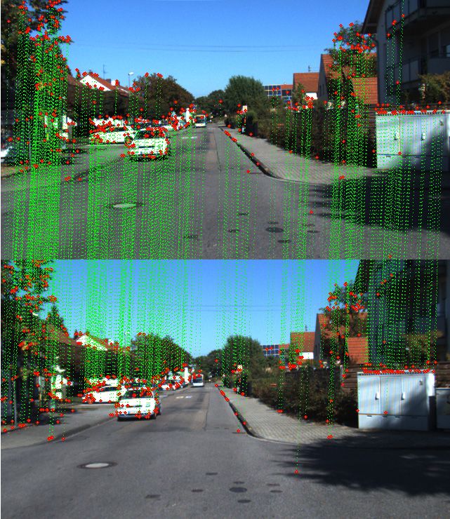
accelerates the operational speed but also reduces the hardware cost. The experiment results show
that the proposed enhanced-SIFT reaches a frame rate of 205 fps for 640 × 480 images. Integrated
with two enhanced-SIFT, a finite-area parallel checking is also proposed without the aid of external
memory to improve the efficiency of feature matching. The resulting frame rate by the proposed
Citation: Kuo, C.-H.; Huang, E.-H.; stereo vision matching can be as high as 181 fps with good matching accuracy as demonstrated in
Chien, C.-H.; Hsu, C.-C. FPGA the experimental results.
Design of Enhanced Scale-Invariant
Feature Transform with Finite-Area Keywords: SIFT; FPGA; feature detection; feature descriptor; feature matching; stereo vision; Epipolar
Parallel Feature Matching for Stereo
Vision. Electronics 2021, 10, 1632.
https://doi.org/10.3390/
electronics10141632 1. Introduction
Recently, vision-based simultaneous localization and mapping (V-SLAM) techniques
Academic Editors: Stefano Ricci and
have become more and more popular due to the need for the autonomous navigation
Akash Kumar
of mobile robots [1,2]. The front-end feature point detection and feature matching are
especially important because their accuracy will significantly influence the performance of
Received: 15 May 2021
Accepted: 7 July 2021
back-end visual odometry, mapping, and pose estimation [3,4]. In the front-end schemes,
Published: 8 July 2021
although speed-up robust features (SURF) exhibit a faster operational speed, its accuracy is
worse than scale-invariant feature transform (SIFT) [5,6]. Nevertheless, the high accuracy
Publisher’s Note: MDPI stays neutral
of SIFT is achieved at the cost of a time-consuming process. Although CUDA implemen-
with regard to jurisdictional claims in
tations on GPUs for parallel programming can be used for various feature detection and
published maps and institutional affil- matching [7,8], the software-based approaches generally require a larger power consump-
iations. tion which is not desired for mobile robot vision applications. Thus, this paper aims to
improve the operational speed of SIFT by hardware implementation without sacrificing
its accuracy. Over the past years, many researchers were devoted to improving the op-
erational efficiency of SIFT [9]. Among them, a pipelined FPGA-based architecture was
Copyright: © 2021 by the authors.
proposed in [10] to process images with double speed at the price of a higher hardware
Licensee MDPI, Basel, Switzerland.
cost. A hardware implemented SIFT was also proposed in [11] to reduce the number of
This article is an open access article
internal registers. However, the resulting image frame rate is not high enough because
distributed under the terms and of finite bandwidth due to external memory. As a result, the efficiency of the subsequent
conditions of the Creative Commons mapping process could be limited. In [12], multiple levels of Gaussian-blurred images
Attribution (CC BY) license (https:// were simultaneously generated by adequately modifying Gaussian kernels to shorten the
creativecommons.org/licenses/by/ processing time, resulting in a frame rate of 150 fps for 640 × 480 images. Although a
4.0/). few dividers were only used by the modified approach for feature detection, the resulting
Electronics 2021, 10, 1632. https://doi.org/10.3390/electronics10141632 https://www.mdpi.com/journal/electronics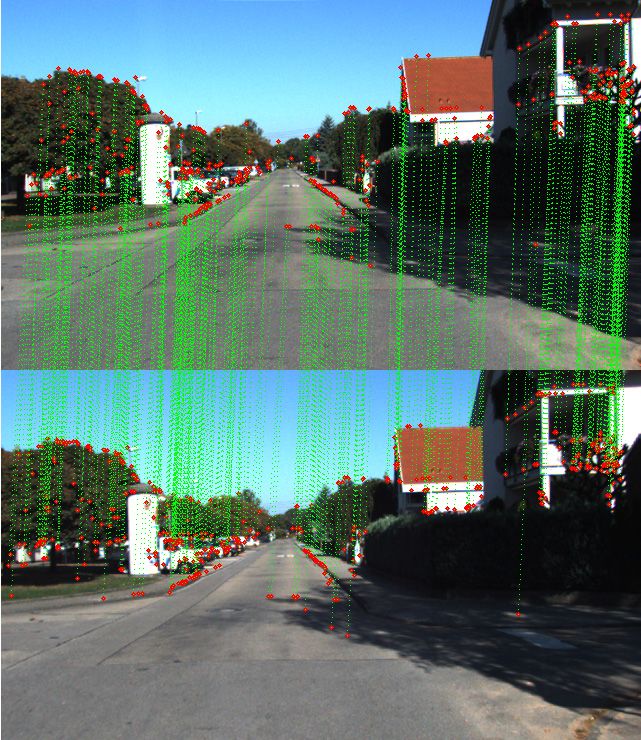
Electronics 2021, 10, 1632                                                                                          2 of 24

                             hardware cost is difficult to reduce because of the square function in the design. Besides,
                             the coordinate rotation digital computer (CORDIC) algorithm adopted in finding phases
                             and gradients of the feature descriptor often requires considerable hardware resources and
                             a long latency period due to the needs of multiple iterations, thus significantly preventing
                             the approach from being applied for real-world applications.
                                  As far as feature matching is concerned, one feature point of an image needs to
                             compare with all feature points of the other image to find the matching pairs [13] in
                             conventional exhaustion methods. A large number of feature points would incur extra
                             memory access time. Moreover, the realization of feature matching often consumes a
                             large number of hardware resources. Although the random sample consensus (RANSAC)
                             algorithm [14] can improve the accuracy of feature matching, the resulting frame rate is
                             only 40 fps. Therefore, it has brought a great challenge to improve the operational speed of
                             the SIFT for use with feature matching.
                                  In this paper, we propose an enhanced-SIFT (E-SIFT) to reduce the hardware resources
                             required and accelerate the operational speed without sacrificing accuracy. Gaussian-
                             blurred images and difference of Gaussian (DoG) pyramids can be simultaneously ob-
                             tained by meticulous design of a realizing structure. We also propose a simple triangular
                             identification (TI) with a look-up table (LUT) to easily and quickly decide the direction and
                             gradient of a pixel point. The resulting dimension of feature points can thus be effectively
                             reduced by half. This is not only beneficial to the operational speed of the proposed E-SIFT
                             and the following feature matching but also helpful to reduce the hardware cost. In the
                             feature detection, the condition of high-contrast detection is also modified by slightly
                             adjusting a threshold value without substantial change, thus considerably reducing the
                             required logic elements and processing time.
                                  For stereo vision, we also propose a finite-area parallel (FAP) feature matching ap-
                             proach integrated with two E-SIFTs. According to the position of the feature point of the
                             right image, a fixed number of feature points in the corresponding area of the left image
                             will be chosen and stored first. Then, feature matching proceeds in parallel to efficiently
                             and accurately find the matching pairs without using any external memory. Based on
                             the Epipolar geometry, a minimum threshold is assigned during feature comparison to
                             avoid matching errors caused by the visual angle difference between the two cameras [15].
                             Besides, a valid signal is designed in the system to prevent the finite bandwidth of external
                             SDRAM or discontinuous image data transmission from corrupting the matching accuracy.
                             In the experiments, we use Altera FPGA hardware platform to evaluate the feasibility
                             of the proposed TI with LUT scheme and test the flexibility of the proposed E-SIFT and
                             double E-SIFT with FAP feature matching.

                             2. Proposed E-SIFT and Fap Feature Matching for Stereo Vision
                                  Figure 1 shows the proposed FPGA-based E-SIFT architecture, where an initial image
                             is convoluted by a meticulous design of Gaussian filters to simultaneously generate a
                             Gaussian-blurred image and DoG pyramid. Through a definite mask in the Gaussian-
                             blurred image, the direction and gradient of each detection point can be determined by
                             the proposed TI with LUT method. The results in each local area are then summed and
                             collected to form a feature descriptor. Since the summations among different partition
                             areas present large differences, values in the feature descriptors will be normalized to
                             acceptable ones by a simple scheme without considerably altering the original character of
                             distribution. At the same time, on the right side in Figure 1, the corresponding detection
                             point in the DoG images will pass through extrema, high contrast, and corner detections
                             to decide whether feature points exist. If the result is positive, a confirmed signal and the
                             corresponding feature descriptor will be delivered to the feature matching module.
Electronics 2021, 10, 1632 3 of 24
Electronics 2021, 10, x FOR PEER REVIEW 3 of 24
Figure
Figure 1.1.Building
Buildingblocks
blocksofofthe
theproposed
proposed E-SIFT.
E-SIFT.
2.1.
2.1.Image
ImagePyramid
Pyramid
The
Thepurpose
purposeofofbuilding
buildingthe theimage
imagepyramid
pyramidisistotofind findout
outfeature
featurepoints
pointsfrom
fromthethe
differences of consecutive scale-spaces. Multi-level Gaussian-blurred
differences of consecutive scale-spaces. Multi-level Gaussian-blurred images are created images are created
one
oneby byone
onethrough
throughaaseries
seriesof ofGaussian
Gaussian functions.
functions. The The speckles
speckles andand interfering
interferingnoises
noisesin
inthe
theoriginal
original image
image cancan therefore
therefore be reduced
be reduced [9]. [9].
Then, Then, the contour
the contour of objects
of objects in the
in the original
original
image is image is vaguely
vaguely outlined outlined
by the by the differences
differences between between the consecutive
the consecutive Gaussian-
Gaussian-blurred
blurred
images.images.
Thus, theThus, the image
image featurefeature
can be can be reserved
reserved to be
to be the the for
basis basis for subsequent
subsequent feature
feature detection. In general, long latency is expected in constructing
detection. In general, long latency is expected in constructing the multi-level Gaussian- the multi-level
Gaussian-blurred
blurred pyramids. pyramids.
Thus, as Thus,
shownasinshown
Figurein2a, Figure
a more 2a,efficient
a more efficient
structurestructure
had beenhad pro-
been
posed by simultaneously convoluting all the Gaussian functions, where suitable suitable
proposed by simultaneously convoluting all the Gaussian functions, where Gaussian
Gaussian
kernels cankernels can beby
be found found by training
training the system
the system with different
with different images images [12].
[12]. To To further
further accel-
accelerate the construction of the DoG pyramid, a simplified structure
erate the construction of the DoG pyramid, a simplified structure is proposed in this is proposed in this
pa-
paper, where new
per, where new kernels
kernels for
for convolution
convolution are are first
firstderived
derivedby bysubtraction
subtractionofoftwo twoadjacent
adjacent
ones
onesasasshown
shownininFigure
Figure2b. 2b.Then,
Then,thethenth
nthlevel
levelDoG image,DnD(x,
DoGimage, y), can be obtained by
n(x, y), can be obtained by
directly convoluting the original image with the
directly convoluting the original image with the new kernel: new kernel:
Dn ( x, y)D= L ( x, y) − L ( x, y) = [ G +n1+(1x,
n ( x ,ny+)1= Ln +1 ( x, y )n− Ln ( x, y ) = [nG ( xy, y) )−− Gnn((xx,, yy)])]∗∗I (Ix(,x,y )y,), (1)(1)
whereLnL(x,
where n(x,
y)y)and
andGG n(x,y)
n (x, y)are
arethe
thenthnthlevel
levelGaussian-blurred
Gaussian-blurredimage imageand andGaussian
Gaussiankernel,
kernel,
respectively,
respectively, andandI(x,I(x,
y) is
y)the initial
is the image.
initial In the
image. In proposed
the proposedstructure, the DoG
structure, the pyramid and
DoG pyramid
the
andrequired Gaussian-blurred
the required Gaussian-blurred image image
can becan
directly createdcreated
be directly at the same
at thetime.
sameHere,
time.only
Here,
the 2ndthe
only level
2ndGaussian-blurred
level Gaussian-blurred image isimage
reserved to be thetobasis
is reserved of the
be the feature
basis of thedescriptor.
feature de-
Since a 7 × 7 mask is adopted mainly for the convolution in the image pyramid,
scriptor.
49 general-purpose
Since a 7 × 7 mask 8-bit registers
is adopted will be required
mainly for the to store the pixel
convolution data.
in the imageForpyramid,
an image49
width of 640 pixels, a large number of 8-bit registers needs be aligned
general-purpose 8-bit registers will be required to store the pixel data. For an image row by rowwidth
for
the serial input of pixel data. To dramatically reduce the number of internal
of 640 pixels, a large number of 8-bit registers needs be aligned row by row for the serial registers, we
propose
input ofa pixel
bufferdata.
structure as shown in
To dramatically Figurethe
reduce 3. number
We utilize of Altera
internaloptimized
registers, RAM-based
we propose a
shift registers
buffer to form
structure a six-row
as shown buffer3.array,
in Figure where Altera
We utilize each row includesRAM-based
optimized 633 registers. Once
shift reg-
the pixel
isters todata
formreaches
a six-row thebuffer
last one, i.e.,where
array, reg. 49, 7 × includes
the row
each 7 convolution can be accomplished
633 registers. Once the pixel
indata
one clock
reachescycle.
the A similar
last buffer
one, i.e., structure
reg. 49, the with
7 × 7 different
convolutionsizescan
for be
theaccomplished
following building
in one
Electronics 2021, 10, x FOR PEER REVIEW 4 of 24
Electronics2021,
Electronics 2021, 10,
10, x FOR PEER REVIEW
1632 4 4ofof2424
clock
clockcycle.
cycle.AAsimilar
similarbuffer
bufferstructure
structurewith
withdifferent
differentsizes
sizesfor
forthe
thefollowing
followingbuilding
buildingblocks
blocks
blocks requiring
requiring acan
mask can also be adopted to efficiently reduce the register number as
requiring a mask can also be adopted to efficiently reduce the register numberasaswell
a mask also be adopted to efficiently reduce the register number wellasas
well as shorten
shorten the buffer delay.
shortenthe
thebuffer
bufferdelay.
delay.
(a)
(a) (b)
(b)
Figure
Figure2.
Figure 2.2.(a)
(a)Conventional
(a) Conventionalstructure
Conventional structureand
structure and(b)
and (b)the
(b) theproposed
the proposedstructure
proposed structure ininrealizing
structurein realizing image
realizingimage pyramids.
imagepyramids.
pyramids.
Figure
Figure3.
Figure 3.3.8-bit
8-bitinput
8-bit inputbuffers
input buffersfor
buffers for777×××777mask.
for mask.
mask.
2.2. Feature Descriptor
Descriptor
2.2.Feature
Feature Descriptor
To accelerate the generating speed of feature descriptors, the direction and gradient
To accelerate the generating speed of feature descriptors, the direction and gradient
of the detection point need to be quickly determined. Thus, Thus, in this paper, the TI method
of the detection point need to be quickly determined. Thus,inin this paper, the TI method
is proposed
proposed to to promptly
promptly determine
determinethe thedirection
directionofofthe thedetection
detection point.CombinedCombined witha
is proposed to promptly determine the direction of the detectionpoint. point. Combinedwith with a
a look-up
look-up table, the gradient of the detection point can be easily estimated. In general,
look-uptable,
table,the
thegradient
gradientofofthe
thedetection
detectionpoint
pointcan canbebeeasily
easilyestimated.
estimated.InIngeneral,
general,eight
eight
eight different
different directions need to be determined to reducecomplexity
the complexity of phase the phase of
differentdirections
directionsneed needtotobebedetermined
determinedtotoreducereducethethe complexityofofthe the phaseofofthethe
the detection
detection pointpoint [9,16].
[9,16]. In In this
this paper,
paper, the the eight
eight directions
directions with with unsigned
unsigned gradients
gradients for for
the
detection point [9,16]. In this paper, the eight directions with unsigned gradients for the
the detection
detection point have been simplified to four with signed ones to reducehardware
the hardware
detectionpoint
pointhave
havebeenbeensimplified
simplifiedtotofour
fourwith
withsigned
signedones
onestotoreduce
reducethethe hardwarecost. cost.
cost. Although
Although the resulting gradient size increases by one bit, the dimension of the feature
feature
Althoughthe theresulting
resultinggradient
gradientsize
sizeincreases
increasesby byone
onebit,
bit,the
thedimension
dimensionofofthe the feature
descriptor can
descriptor can be
be effectively reduced
reduced by half.
half. It is also helpful
helpful to the FAP FAP feature matching
matching
descriptor
for can beeffectively
implementation. effectively reducedby by half.ItItisisalso
also helpfultotothe the FAPfeature
feature matching
for
forimplementation.
implementation.
Figure 44 shows
Figure showsthe theblock
blockdiagram
diagram of thefeature
featuredescriptor.
descriptor.First, First, 3a×33×mask
3 mask is
applied Figure
to the4 2nd
shows level block diagramofofthe
theGaussian-blurred the feature
image to finddescriptor.
the First,abetween
differences a 3 × 3 mask isisap-
adjacentap-
plied
pliedtoin
tothe 2nd level
levelGaussian-blurred image
imagetotofindfindthethedifferences between adjacent
pixels xthe
and2ndy axes toGaussian-blurred
the center. The direction and differences
gradient between
of the center adjacent
point will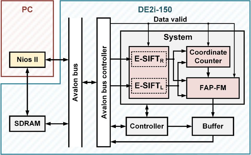
scriptor of the detection point can be synthesized by finding and collecting g
of the four directions in each 4 × 4 partition area of a 16 × 16 mask.
Electronics 2021, 10, x FOR PEER REVIEW 5 of 2
Electronics 2021, 10, 1632 5 of 24
pixels in x and y axes to the center. The direction and gradient of the center point will the
thendetermined
be be determined respectively
respectivelyby
bythe
the proposed
proposed TI TIwith
withLUT
LUT method.
method. Finally,
Finally, the feature de
the feature
scriptor ofofthe
descriptor thedetection
detection point
point can
can bebe synthesized
synthesizedby byfinding
findingand
and collecting
collecting gradient sum
gradient
sums
of theoffour
the four directions
directions in each 4 ×4 4×partition
in each 4 partitionarea
areaof
ofaa 16 ×16
16 × 16 mask.
mask.
Figure 4. Function blocks of the feature descriptor.
2.2.1. Triangular Identification and Look-Up Table
In4.4.conventional
Figure
Figure Function
Function blocks
blocks approaches,
of the
of the feature
feature the center
descriptor.
descriptor. point, i.e., L2(x, y), of every 3 × 3 m
in2.2.1.
the 2nd level Gaussian-blurred image is the detection point. The variatio
2.2.1.Triangular
TriangularIdentification and and
Identification Look-Up
Look-UpTable Table
tection point on x and y axes, i.e., Δp and Δq, are defined by the differences
In conventional approaches, the center point, i.e., L2 (x, y), of every 3 × 3 mask shifting
adjacent In conventional approaches, thein
center point,
5. i.e.,point.
L2(x, y), of every 3 × 3 mask shiftin
in the 2ndpixel values, as shown
level Gaussian-blurred image isFigure
the detection The variations of the
in the 2nd
detection level
point on xGaussian-blurred image
and y axes, i.e., ∆p and ∆q, is
arethe detection
defined by thepoint. The variations
differences between twoof the de
tection point
adjacent on x and
pixel values, y axes,ini.e.,
as shown Δp Δ
Figure and
5. p =Δq, x +defined
L2 (are 1, y ) − Lby
2 ( x − 1, y )
the differences between tw
adjacent pixel values, as shown in Figure 5.
∆p = L2 ( x + 1, y) − L2 ( x − 1, y) (2)
Δp =ΔLq2 (=x +L1, (yx) ,−yL+ x −−1,Ly ) ( x, y − 1)
2 (1) (2
2 2
∆q = L2 ( x, y + 1) − L2 ( x, y − 1) (3)
Δq = L2 ( x, y + 1) − L2 ( x, y − 1) (3
Figure 5. Variations of the detection point on x and y axes in a 3 × 3 mask.
Figure 5. Variations of the detection point on x and y axes in a 3 × 3 mask.
Figure 5. Variations of the detection point on x and y axes in a 3 × 3 mask.
Since these two variations are perpendicular to each other, the resulting phase an
Since these
magnitude whichtwo variations
define areand
the direction perpendicular
gradient of thetodetection
each other,
pointthe
can resultin
be easil
determined by the following equations [9].
magnitude which define the direction and gradient of the detection point
Δq
θ ( x, y ) = arctan (4)
Δp
Electronics 2021, 10, 1632
m( x, y) = Δp 2 + Δq 2 6 of 24
(5)
Conventional approaches generally utilize the CORDIC algorithm to derive the re-
sults of Equations (4) and (5) [17]. However, time-consuming and tedious procedures
Since due
would ensue thesetotwo variations
a large numberare ofperpendicular
iterations. In this to each other,
paper, we the resulting
propose phaseTIand
a simple
magnitude which define the direction and gradient of the detection
method to determine the phase of detection points. Since only eight directions exist in point can bethe
easily
determined by the following equations [9].
original definition, the direction of the detection point can be easily determined by the
value of Δp and Δq, which are two legs of a right-angled
∆q triangle. For example, if Δp is
θ ( x, y ) =
larger than Δq, and both are greater than zero, then the hypotenuse will be located in (4)
arctan
∆p
direction 0, as shown in Figure 6a. Thus, the direction of the detection point is classified
as phase 0 directly. Conversely, the direction of the detection point is classified as phase 1
q
m( x, y) = ∆p2 + ∆q2 (5)
if Δp is smaller than Δq. In a similar way, we can easily recognize other different directions
by usingConventional
Table 1. The approaches
required conditions
generallyare alsothe
utilize devised
CORDIC to distinguish
algorithm todifferent
derive thedirec-
results
tions.
of Absolute
Equationsvalues
(4) and are(5)
considered in reality
[17]. However, because the lengths
time-consuming of bothprocedures
and tedious legs cannotwouldbe
negative.
ensue due to a large number of iterations. In this paper, we propose a simple TI method to
For a right-angled
determine the phasetriangle, if there
of detection is a big
points. difference
Since only eight between the length
directions exist inofthe
theoriginal
two
legs,definition,
the hypotenuse length of
the direction can bedetection
the approximated as the
point can be longer one. If two legs
easily determined by thehave equal
value of ∆p
and ∆q,
lengths, i.e.,which
Δp = Δq,arethe
two hypotenuse length will be
legs of a right-angled 2
triangle. times
For leg one,
example, as
if ∆p
shown
is in
largerFigure
than ∆q,
and both
6b. Thus, the are greaterofthan
gradient zero, thenpoint
the detection the hypotenuse will be located
cannot be directly estimatedin direction
only by the 0, as shown
com-
in Figure
parison of the6a.
twoThus, the direction
legs. Here, a look-upoftablethe detection
is proposed point is classified
for the estimationasofphase 0 directly.
the gradient
Conversely,
of the detectionthe direction
point, of the
as listed in detection pointthe
Table 2. First, is classified
ratio, h, of phase 1 if ∆p
as variations is smaller
in two axes isthan
∆q. In afor
evaluated similar way, the
choosing we can easily recognize
correction factor, K,other different
as shown directions
in the table. Theby gradient
using Table 1. The
of the
required conditions are also devised to distinguish different directions.
detection point, m, will then be approximated by the length of the longer leg multiplied Absolute values
by aare considered
chosen in reality
correction factor.because the lengths of both legs cannot be negative.
(a) (b)
Figure 6. (a)6.The
Figure proposed
(a) The TI algorithm
proposed for direction
TI algorithm recognition;
for direction (b) The
recognition; ratioratio
(b) The of hypotenuse to the
of hypotenuse to the
leg has maximum
leg has maximum value when
value Δp =∆p
when Δq.= ∆q.
Table 1. Angle
Table range
1. Angle condition
range andand
condition direction distribution.
direction distribution.
Direction Direction Conditions Conditions Pixel
PixelPhase
Phaseθθ
0 0 Δp > 0, Δq ∆p > 0, ∆q ≥ 0> &
≥ 0 & |Δp| |Δq|
|∆p| > |∆q| ∠θ
0°0◦≤ ≤ ∠θ˂ 0, Δq ∆p > 0, ∆q > 0 &|Δq|
> 0 & |Δp| ≤ |∆p| ≤ |∆q| 45° ≤
◦ ∠ θ ˂
45 ≤ ∠θ < 90◦90°
2 2 Δp ≤ 0, Δq ∆p ∆q > 0< &
> 0≤&0,|Δp| |Δq|
|∆p| < |∆q| 90◦≤ ≤
90° ∠θ 135◦
∠θ˂ 0≥&|Δq|
> 0 |∆q| 180 ≤ ∠θ < 225
4 Δp < 0, Δq ≥ 0 & |Δp| > |Δq| 180° ◦≤ ∠θ ˂ 225°◦
5 ∆p < 0, ∆q < 0 & |∆p| ≤ |∆q| 225 ≤ ∠θ < 270
5 6 Δp < 0, Δq ∆p
< 0≥&0,|Δp|
∆q < 0≤ &
|Δq|
|∆p| < |∆q| 225°
270◦≤≤ ∠θ∠θ˂
Electronics 2021, 10, 1632                                                                                                         7 of 24
 Electronics 2021, 10, x FOR PEER REVIEW                                                                                             7 of 24

                                  gradient
                                        Noteof that
                                                the detection
                                                      the featurepoint,    m, willrequires
                                                                     descriptor     then beeight
                                                                                             approximated
                                                                                                 dimensions bytothe lengthdifferent
                                                                                                                  express  of the longer
                                                                                                                                    gradi-
                                  leg multiplied     by  a  chosen   correction  factor.
                                   ents of the eight directions. To reduce hardware resources, a representation having fewer
                                   dimensions is discussed in this paper. From the observation of Figure 6, phase 4 has an
                                  Table 2. Look-up
                                   opposite  direction tabletofor gradient
                                                                phase      correction.phase 5 has an opposite direction to phase 1, and
                                                                       0. Similarly,
                                   so on. Thus, the eight-direction representation can be simplified to a four-direction one to
                                            h = |∆p/∆q|                       Correction Factor (K)             Pixel Gradient (m)
                                   reduce the resulting dimensions. For example, if the detection point has an unsigned gra-
                                               h ≤ 0.25
                                   dient in phase     4, it will be changed to have1.00  a negative one in phase 0. As shown in Figure
                                           0.25 < h ≤ 0.52                             1.08
                                   7, the proposed       TI
                                           0.52 < h ≤ 0.65   with  LUT   approach    for detecting
                                                                                       1.17        the direction and gradient of the de-
                                   tection 0.65
                                            point    is  processed
                                                 < h ≤ 0.75           in parallel  to accelerate
                                                                                       1.22      the operational speed. The presented
                                   structure  is
Electronics 2021,
Electronics 10, x1632
2021, 10, FOR PEER REVIEW 88of
of24
24
will possess
sentation will64possess
dimensions, which are which
64 dimensions, half of are
thathalf
by conventional methods, as
of that by conventional shown in
methods, as
Figure
shown8b.in It not only
Figure reduces
8b. It thereduces
not only required devices
the in implementation
required but also accelerates
devices in implementation but also
the producing
accelerates thespeed of feature
producing speeddescriptors. These benefits
of feature descriptors. arebenefits
These also helpful to the
are also subse-
helpful to
quent feature matching.
the subsequent feature matching.
(a) (b)
Figure
Figure 8.
8. (a)
(a)Sixteen
Sixteen 44 ××4 4partitions
partitionsininaa16
16××
1616
mask
maskfor
forthe
thefeature
featuredescriptor
descriptorand
and(b)
(b)the
thecorresponding
correspondinggradient
gradientsum
sumin
in
each 4 × 4 partitions.
each 4 × 4 partitions.
2.2.3.
2.2.3.Normalization
Normalization
For
For general
general images, images, large differences
differencesusually
usuallyexist
existamong
amongthe
thegradient
gradientsums,
sums, result-
resulting
ing in different
in different dimensions
dimensions ofof thefeature
the featuredescriptor.
descriptor. Consequently,
Consequently, the feature
featuredescriptor,
descriptor,
OF
OF == (o
(o11, , oo22, ,…,
. . . o, 64o), needs
64 ), needstotobebenormalized
normalizedtotodecrease
decreasethe
thescale
scale without
without significantly
significantly
altering distributionamong
altering the distribution amonggradient
gradient sums.
sums. TheThe normalization
normalization of theoffeature
the feature de-
descriptor
scriptor
is achievedis achieved
in this paper in thisby:
paper by:
OF
F = ( f , f , , f ) = R × OF (6)
F = ( f 1 , 1f 2 , 2· · · , f 6464) = R ×W (6)
W
where W is the sum of all gradient sums in all dimensions of the feature descriptor.
where W is the sum of all gradient sums in all 64 dimensions of the feature descriptor.
W = oi (7)
64
i =1
W = ∑ oi (7)
A scaling factor, R = 255, is chosen here for better discrimination. That is, the resulting
i =1
gradient sums of the feature descriptor lie between ±255. Thus, the required bit number
of theAgradient sum isRreduced
scaling factor, = 255, is from
chosen13here
bitsfor
to better
9 bits discrimination. That is,
in the normalization ofthe
theresulting
feature
gradient sums of the feature descriptor lie between ±
descriptor. In the implementation of the presented normalization, we introducenumber
255. Thus, the required bit an addi-of
the gradient sum is reduced from 13 bits to 9 bits in the normalization of
tional multiplier having the power of 2 approximating the sum of all gradients for achiev- the feature de-
scriptor.
ing In the
a simple implementation
operation. Thus, theof normalized
the presented normalization,
feature descriptorweF introduce an additional
can be easily obtained
multiplier
by having
only shifting bitsthe
of power of 2 approximating
the feature descriptor. The the sum of
realized all gradients
block diagram of forthe
achieving
normali-a
simple operation. Thus,
zation is shown in Figure 9. the normalized feature descriptor F can be easily obtained by only
shifting bits of the feature descriptor. The realized block diagram of the normalization is
R×2j 1
shown in Figure 9. F= × OF × j (8)
R ×W2 j 21
F= × OF × j (8)
W 2
Electronics 2021, 10, 1632 9 of 24
Electronics 2021, 10, x FOR PEER REVIEW 9 of 24
Figure9.9.Function
Figure Functionblocks
blocksofofthe
thenormalization
normalizationofofthe
thefeature
featuredescriptor.
descriptor.
2.3.
2.3.Feature
FeatureDetection
Detection
Electronics 2021, 10, x FOR PEER REVIEW 10 of 24
In the beginning, we use
In the beginning, we use three
threelevels
levelsofofDoGDoGimages
imagesto to establish
establish a 3Da 3D space.
space. A 3 ×A3
3 × 3 mask will then be applied to the three DoG images to define 27-pixel data for feature
mask will then be applied to the three DoG images to define 27-pixel data for feature de-
detection, as shown in Figure 10. Thus, center pixel of the 3 × 3 mask in the 2nd level DoG
tection, as shown in Figure 10. Thus, center pixel of the 3 × 3 mask in the 2nd level DoG
image, D2, is regarded as the detection point. Three kinds of detections, including extrema
( x, y +
image, D2, is regarded as theDdetection − D1 ( xThree
1) point. + 1)kinds
, ydetection,
D (of − 1) − D1 (and
x, detections,
y adopted , y −processed
xincluding
1) extrema
detection, high contrast
detection, high contrast ≡ 3
Dyzdetection,
detection,
and corner − 3 are
and4 corner detection, are adopted and processed
in
in (16)
parallel, as shown in Figure 11. 4
parallel, as shown in Figure 11.
Once the results of the three detections are all positive, the detection point becomes
a feature point, and a detected signal will be sent to the feature descriptor and feature
matching blocks for further processing.
To evaluate the variation of the pixel values around the detection point, 3D and 2D
Hessian matrix, H3×3 and H2×2, respectively, will be used in the high contrast and corner
detections.
Dxx Dxy
H 2×2 = (9)
Dxy Dyy
Dxx Dxy Dxz
H 3×3 = Dxy Dyy Dyz , (10)
Figure 10.The
Figure 10. Thedetection
detection range
range includes
includes 27 D
pixels
27 pixels Din
xzin three Dzz images
yz three
DoG DoG images
under aunder a 3 × 3where
3 × 3 mask, mask, where
the
the orange
orange pixel
pixel isis regarded
regarded as as
the the detection
detection point.
point.
where the definitions of the elements are listed as follows.
Once the results of the D xx ≡ D
three 2 ( x + 1, y ) +are
detections x −positive,
D2 (all 1, y ) − 2 D2the
( x, detection
y) point becomes
(11)
a feature point, and a detected signal will be sent to the feature descriptor and feature
matching blocks for furtherD processing.
yy ≡ D2 ( x, y + 1) + D2 ( x, y − 1) − 2D2 ( x, y) (12)
To evaluate the variation of the pixel values around the detection point, 3D and
2D Hessian matrix, H3×3 and H2×2 , respectively, will be used in the high contrast and
Dzz ≡ D3 ( x, y ) + D1 ( x, y ) − 2 D2 ( x, y ) (13)
corner detections.
Dxx Dxy
D2 ( x + 1, y + 1)H−2× x + 1, D
D22 (= y − 1) DD2 ( x − 1, y + 1) − D2 ( x − 1, y − 1) (9)
Dxy ≡ xy − yy (14)
4 4
Dxx Dxy Dxz
D ( x + 1, y ) − D ( x + 1, y) D ( x − 1, y) − D1 ( x − 1, y)
Dxz ≡ 3 H3×3 = 1Dxy Dyy− 3Dyz , (10)
(15)
4 Dxz Dyz Dzz 4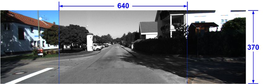
Electronics 2021, 10, x FOR PEER REVIEW                                                                                                        10 of

                                                                  D3 ( x, y + 1) − D1 ( x, y + 1) D3 ( x, y − 1) − D1 ( x, y − 1)
 Electronics 2021, 10, 1632                               Dyz ≡                                  −                                  10 of 24
                                                                                                                                                  (1
                                                                                 4                               4

                                 where the definitions of the elements are listed as follows.

                                                         Dxx ≡ D2 ( x + 1, y) + D2 ( x − 1, y) − 2D2 ( x, y)                           (11)

                                                         Dyy ≡ D2 ( x, y + 1) + D2 ( x, y − 1) − 2D2 ( x, y)                           (12)
                                                             Dzz ≡ D3 ( x, y) + D1 ( x, y) − 2D2 ( x, y)                               (13)
                                           D2 ( x + 1, y + 1) − D2 ( x + 1, y − 1)  D ( x − 1, y + 1) − D2 ( x − 1, y − 1)
                                   Dxy ≡                                           − 2                                                 (14)
                                                              4                                       4
                                                      D3 ( x + 1, y) − D1 ( x + 1, y)  D ( x − 1, y) − D1 ( x − 1, y)
                                              Dxz ≡                                   − 3                                              (15)
                                                                     4                               4
                                                     D ( x, y + 1) − D1 ( x, y + 1)  D3 ( x, y − 1) − D1 ( x, y − 1)
                                  Figure 10. The ≡ 3
                                             Dyz detection   range includes 27 pixels
                                                                                    − in  three DoG images under a 3 × 3(16)
                                                                                                                          mask, whe
                                                                   4                                4
                                  the orange pixel is regarded as the detection point.

                                  Figure
                                 Figure 11.11. Building
                                            Building    blocks
                                                     blocks      offeature
                                                            of the  the feature detection.
                                                                           detection.

                                      Since both
                                        Since    thethe
                                              both    matrices
                                                        matricesareare
                                                                    symmetric,  only
                                                                       symmetric,     six six
                                                                                   only   elements needneed
                                                                                              elements   to betodetermined.
                                                                                                                 be determined. Fig
                                 Figure
                                  ure 12 shows the realized structure, where pixel inputs come fromcorresponding
                                        12 shows  the realized structure, where pixel  inputs come from the  the corresponding p
                                 positions shown in
                                  sitions shown   in Figure
                                                     Figure10.
                                                             10.
                                 2.3.1. Extreme Detection
                                      In extreme detection, the detection point is compared with the other 26 pixels in the
                                 3D mask range. If the pixel value of the detection point is the maximum or the minimum
                                 one, the detection point will be a possible feature point [18].
Electronics
Electronics 2021,
2021, 10,10,x 1632
FOR PEER REVIEW 11 of 24 11 of 24
12.Hardware
Figure 12.
Figure Hardwarestructure of the
structure elements
of the in 2Dinand
elements 2D3D Hessian
and matrices.
3D Hessian matrices.
2.3.2. High Contrast Detection
2.3.1.InExtreme Detection
conventional approaches, when the variation of the pixel values in three-dimension
spaceInaround
extremethedetection, the detection
detection point is greaterpoint
than is comparedofwith
a threshold 0.03, the
the other 26 pixels in the
high contrast
feature
3D maskcanrange.
be assured
If the[11].
pixelHere,
valueto of
simplify the derivations
the detection point isand
thesubsequent
maximumhardware
or the minimum
design,
one, thean approximated
detection point value of a1/32
will be is chosen
possible to be
feature the threshold
point [18]. value. That is, the
resulting pixel variation criterion is modified as:
2.3.2. High Contrast Detection 1
| D (S)| > , (17)
In conventional approaches, when the 32 variation of the pixel values in three-dimen-
sion space around the detection point is greater than a threshold of 0.03, the high contrast
where S = [x y z]T denotes the 3D coordinate vector. The pixel variation can be expressed
feature can be assured [11].
as the Maclaurin series and Here, to simplify
approximated by: the derivations and subsequent hardware
design, an approximated value of 1/32 is chosen to be the threshold value. That is, the
T (0) 1 T ∂2 D (0)
resulting pixel variation criterion is∂D
modified as:
D ( S ) ≈ D (0) + ·S+ S · ·S (18)
∂S 2 1 ∂S2
D(S ) > , (17)
where D(0) represents the pixel value of the detection32point. The transpose of the partial
derivative
where [xD(0)
S =of y z]Twith respect
denotes the S will
to3D be:
coordinate vector. The pixel variation can be expressed
as the Maclaurin series
and approximated
T T by:
∂D (0) ∂D (0)
= =T [ Dx Dy Dz 2], (19)
∂S ∂D (0) 1 ∂ D (0)
⋅ S + ST ⋅
∂S
D ( S ) ≈ D (0) + ⋅S (18)
∂S 2 ∂S 2
where
where D(0) represents D2pixel
the y) − D
( x + 1,value x − detection
of2 (the 1, y) d − D2 fThe transpose of the partia
D point.
Dx ≡ = 2 (20)
derivative of D(0) with respect( xto − ( xbe:
+ 1S)will − 1) 2
D2 ( x, y + 1) −T D2 ( x,Ty − 1)
Dy ≡ ∂D(0) ∂D (0) = D2 b − D2 h , (21)
(y + 1) − (y − 1) = [ Dx Dy2 Dz ]
∂S
=
∂S
(19)
D3 ( x, y) − D1 ( x, y) D e − D1 e
where and Dz ≡ = 3 . (22)
3−1 2
Figure 13 shows D D2 ( x +hardware
the ≡realized 1, y) − D2 ( of
x −the
1, ypartial − D2f
) D2dderivative. The second partial
= (20)
derivative of D(0) is the xsame as the
( x + 1) − ( x − 1)
3D Hessian matrix. 2
D2 ( x, y + ∂1)2 D
− (D02)( x, y − 1) D2b − D2h
Dy ≡ 2
= H3×3 = (23) (21)
( y + 1) − ( y − 1)
∂S 2
and Dz ≡ D3 ( x , y ) − D1 ( x , y ) = D3e − D1e . (22)
3 −1 2
Figure 13 shows the realized hardware of the partial derivative. The second partia
derivative of D(0) is the same as the 3D Hessian matrix.
∂ 2 D (0)
= H 3×3 (23)
∂S 2Electronics 2021,
Electronics 10,10,x 1632
2021, FOR PEER REVIEW 12 of 24
Figure
Figure Hardware
13.13. architecture
Hardware of partialofderivative
architecture of D(0).
partial derivative of D(0).
Let the first derivative of Equation (18) with respect to S equals zero.
Let the first derivative of Equation (18) with respect to S equals zero.
D 0 (S) = 0 (24)
D′( S ) = 0
The most variation of the pixel values around the detection point can be found at:
The most variation of the pixel values around the detection point can be fou
∂D (0)
S = −( H3×3 )−1 · − 1 ∂D (0)
(25)
S = −(H ∂S
3×3 ) ⋅
∂S
Substituting Equation (25) into Equation (18), we obtain:
∂D T (0) Substituting ∂D (Equation (25) into ∂DEquation
(0) T (18), we obtain:
0) 1 ∂D (0)
D ( S ) = D (0) − · ( H3×3 )−1 · + ( H3×3 )−1 · · H3×3 · ( H3×3 )−1 · T
T
∂S ∂∂SD (0)2 ∂D∂S(0) 1 ∂D(0) ∂S −1 ∂D(
D( S ) = D(0) −
1 ∂D T (0)
⋅(H 3×3 )−1 ⋅ +
3×3 ( H )−1 ⋅ ⋅ H 3×3 ⋅ ( H 3×3 ) ⋅
= D (0) − ∂S · ( H3×3 )−1 · ∂S . 2 ∂S ∂S
∂D (0)
(26)
2 ∂S ∂S
T
1 ∂Dwe
Substituting Equation (26) into Equation (17), (0)
have: −1 ∂D(0) .
= D(0) − ⋅ ( H 3×3 ) ⋅
1 ∂D T (0)
2 ∂S
∂D (0) 1
∂S
D (0) − · ( H3×3 )−1 · >
Substituting Equation (26)
2 ∂S into Equation (17),
∂S we
32 have:
T
∂D T (01) ∂D (0) ∂D (−01) ∂D(0) 1
D(0) − · ( H3×3 )⋅−(1H· 3×3 ) ⋅ > 1 >
⇒ 16 × 2D (0) − (27)
∂S 2 ∂S ∂S ∂S 32
Since the matrix inversion, (H3×3 )−1 , requires lots of dividers in implementation, the
T
16 × 2 D(0) − ∂D (0) ⋅ ( H )−1 ⋅ ∂D(0) 3×>31
resulting hardware cost would be high. Thus, the adjugate matrix, Adj(H ), and the
3×3
determinant, det(H3×3 ), are utilized here to accomplish the matrix inversion instead of
∂S ∂S
using dividers.
Since the matrix inversion, 1 3×3Adj ( H3×3 )
( H3×3 )−(H = )−1, requires , lots of dividers in implementa
(28)
det( H3×3 )
resulting hardware cost would be high. Thus, the adjugate matrix, Adj(H3×3), an
where
terminant, det(H3×3), are utilized here to accomplish the matrix inversion instead
dividers. Dyy Dyz Dxy Dxz Dxy Dxs
+ Dyz − +
Dzz Dyz Dzz
Adj
D
H3×D3 yy ( ) Dyz
−1 D
( )
Dxy
− Dxz
Dyz
+H3×3
D xx = xz xx, Dxz
Adj( H3×3 ) = −
Dxz Dzzdet H3×3Dxy ( ) (29)
Dzz Dyz
Dxy Dyy Dxx Dxy Dxx Dxy
where + − +
Dxz Dyz Dxz Dyz Dxy Dyy
and D yy D yz Dxy Dxz Dxy Dxs
+D D D− +
Dxxyz Dxyzz xzD
yz Dzz Dyy Dyz
det( H3×3 ) = Dxy Dyy Dyz (30)
DDxzxy DDyzyz DzzDxx Dxz Dxx Dxz
Adj ( H 3×3 ) = − + −
Dxz Dzz Dxz Dzz Dxy Dyz
Dxy Dyy Dxx Dxy Dxx Dxy
+ − +
Dxz D yz Dxz Dyz Dxy Dyy
andElectronics 2021, 10, x FOR PEER REVIEW 13 of 24
Figure 14 shows the realized architecture of the determinant and adjugate matrices.
Electronics 2021, 10, 1632 13 of 24
Since the adjugate matrix is symmetric, only six elements need to be processed in the im-
plementation. The determinant of H3×3 can be obtained by repeatedly using the first row
of the adjugate matrix combined with elements in the first column of the determinant to
reduce the hardware
Figure 14 showscost. Thus, Equation
the realized (27) can
architecture of be
therewritten
determinantas: and adjugate matrices.
Since the adjugate matrix is symmetric, onlyAdj
∂DT (0) six( Helements need to be processed in the
3×3 ) ∂D (0)
16 × 2 D(0)of
implementation. The determinant − H3×3 can ⋅ be obtained ⋅ by>repeatedly
1 using the first
∂S det( H 3×3 ) ∂S
row of the adjugate matrix combined with elements in the first column of the determinant (31)
to reduce the hardwarecost. Thus, Equation (27) can be rewritten
16 × 2 D (0) ⋅ det ( H ) − Mul > det ( H ) , as:
3×3 3×3
where ∂D T (0)Adj( H3×3 ) ∂D (0)
16 × 2D (0) − · · >1
∂
∂SD (0)Tdet( H3×3 ) ∂D(0) ∂S (31)
Mul = ⋅ Adj ( H 3×3 ) ⋅ (32)
⇒ 16 × |2D (0) · det(∂HS3×3 ) − Mul | > |det∂S ( H 3×3 )| ,
That is, the detection point will have a high-contrast feature and could be regarded
where
as a possible feature point when Equation
∂D T (0(31)
) is satisfied. Since ∂D (0the
) condition for the high-
contrast feature detection⇒isMul
less =
complicated
∂S
· Adj ( H3the
than ·
×3 )conventional
∂S
(32)
ones, the resulting
hardware circuits will be simpler for achieving a higher operating speed [12].
Figure 14.
Figure 14. Hardware architecture of the
the determinant
determinant and
andadjugate
adjugatematrices.
matrices.
2.3.3.That is, the
Corner detection point will have a high-contrast feature and could be regarded
Detection
as a possible
In this paper, thepoint
feature Harriswhen
cornerEquation
detection(31) is satisfied.
is adopted [19], Since the condition for the
high-contrast feature detection is less complicated than the conventional ones, the resulting
2 2
hardware circuits will be simpler r × tr H 2×2 ) > (r +a1)higher
for( achieving ⋅ det( Hoperating
2×2 ) speed [12]. (33)
whereCorner
2.3.3. the parameter
Detectionr is the ratio of two eigenvalues of H2×2 and r > 1, and tr(H2×2) and
det(H2×2) respectively represent the trace and the determinant of H2×2, which are given by:
In this paper, the Harris corner detection is adopted [19],
tr ( H 2×2 ) = Dxx + Dyy (34)
r × tr2 ( H2×2 ) > (r + 1)2 · det( H2×2 ) (33)
Dxx Dxy
and det ( H ) = = Dxx Dyy of 2
− DHxy (35)
where the parameter r is the ratio
2×2 of two eigenvalues
Dxy Dyy 2×2 and r > 1, and tr(H 2×2 )
and det(H2×2 ) respectively represent the trace and the determinant of H2×2 , which are
givenThat
by: is, the detection point has a corner feature if the inequality Equation (33) is sat-
isfied. An empirical value, r = 10,tris( Hchosen here for acquiring a better result. Figure (34)
2×2 ) = Dxx + Dyy
15
shows the hardware architecture of the corner detection.
Once the results of det
the(three Dxx are
Dxyall positive, the detection
and H2×2 )detections
= = Dxx Dyy − Dxy 2 point will (35)
be
logically regarded as a feature point. During D Dyyserial input
xy the of pixels, the production of
the feature
That is,descriptor and the
the detection feature
point has apoint detection
corner featureproceeds until no Equation
if the inequality image pixel
(33)re-is
mains.
satisfied. An empirical value, r = 10, is chosen here for acquiring a better result. Figure 15
shows the hardware architecture of the corner detection.Electronics 2021, 10, 1632 14 of 24
Electronics 2021, 10, x FOR PEER REVIEW 14 of 24
Electronics 2021, 10, x FOR PEER REVIEW 14 of 24
Figure
Figure 15. Hardwarestructure
15. Hardware structureofof the
the corner
corner detection.
detection.
Once the Parallel
3. Finite-Area results Matching
of the three
fordetections are all positive, the detection point will be
Stereo Vision
logically
A double E-SIFT with FAP feature matchingserial
regarded as a feature point. During the systeminput of pixels,for
is proposed theuse
production
in stereo of the
feature
vision, as shown in Figure 16. The stereo vision captures images by parallel cameras remains.
descriptor and the feature point detection proceeds until no image pixel for
the left15.
Figure and right E-SIFTs
Hardware respectively
structure of the cornerto find the feature points and the corresponding
detection.
3.feature
Finite-Area Parallel
descriptors, Matching
FL and forsame
FR. At the Stereo Visionthe corresponding coordinates will
moment,
3. Finite-Area
be output by aParallel
A double counterMatching
E-SIFT with FAPfor
triggered by Stereo
the
feature Visionsignals,
detected
matching dtcL and
system dtcR, fromfor
is proposed theuse
twoin E- stereo
SIFTs.AThen,
vision, as theE-SIFT
shown
double stereo matching
in Figure
with16.FAPThepoints, MX
stereo
feature L, MYL
vision
matching , MX R, and
captures
system is MY
images R, will
proposed beforfound
by parallel out
usecameras
in andfor the
stereo
recorded
left and as
vision, by
right the
shown proposed
E-SIFTs FAP
respectively
in Figure feature
16. The matching.
to find
stereo Since points
the feature
vision captures theimages
image
andbytransmission
the could for
corresponding
parallel cameras befeature
interrupted
the left anddue
descriptors, right
FL toE-SIFTs
and the
FR.finite bandwidth
Atrespectively
the of find
to
same moment, SDRAM the or noisepoints
the feature coupling,
corresponding and athedata
coordinates valid signal
corresponding
will be output
is
by added
feature to alarm
descriptors,
a counter allFL
triggered building
and blocks
FR.
by the At thetosame
detected prevent abnormal
moment,
signals, dtcLthe termination
dtcR , fromor
andcorresponding the any discontinu-
coordinates
two will Then,
E-SIFTs.
ous
be situation
output by from
a corrupting
counter correct
triggered by output
the messages.
detected signals, dtc and dtc , from the two E-
the stereo matching points, MXL , MYL , MXR , and MYR , will be found out and recorded
L R by
SIFTs. Then, the stereo matching points, MX L, MYL, MXR, and MYR, will be found out and
the proposed FAP feature matching. Since the image transmission could be interrupted
recorded
due to theby the proposed
finite bandwidth FAPof feature
SDRAM matching.
or noiseSince the image
coupling, a datatransmission
valid signal could be
is added to
interrupted due to the finite bandwidth of SDRAM or noise coupling,
alarm all building blocks to prevent abnormal termination or any discontinuous situation a data valid signal
is added to alarm all building blocks to prevent abnormal termination or any discontinu-
from corrupting correct output messages.
ous situation from corrupting correct output messages.
Figure 16. Building blocks of the proposed E-SIFT and FAP feature matching for stereo vision.
Figure 16. Building blocks of the proposed E-SIFT and FAP feature matching for stereo vision.
Figure 16. Building blocks of the proposed E-SIFT and FAP feature matching for stereo vision.Electronics 2021, 10, x FOR PEER REVIEW 15 of 24
Electronics 2021, 10, 1632 15 of 24
3.1. Finite-Area Parallel Feature Matching
3.1. Finite-Area Parallel Feature Matching
Suppose two cameras, CL and CR, are set up in parallel at the same height without
Suppose
any tilt angle two cameras,
difference, CLthree
and and C R , are set
objects, P1, up
P2, in P3,parallel at the
are placed in same height
line with thewithout
right cam-any
tilt
era, as shown in the top view in Figure 17a [20]. In theory, the projections of the sameas
angle difference, and three objects, P 1 , P 2 , P 3 , are placed in line with the right camera,
shown in thetwo
object onto topimage
view in Figure
planes 17abe[20].
will In theory,
on the same row. the projections
However, based of the same object onto
on Epipolar ge-
two image planes will be on the same row. However, based on Epipolar
ometry [15], the imaging of P2 and P3 in the right image could disappear due to the shading geometry [15], the
imaging of P2 by
effect caused andP1P. 3As
in shown
the rightin image
Figurecould disappear
17b, three due to
imagings, P1Lthe shading
, P2L , and P3Leffect caused
, appear in
by P . As shown in Figure 17b, three imagings,
1 image, but only one projection, P1R, in the right
the left P 1L , P , and P ,
one. Therefore,
2L 3L appear in the left image,
to avoid the feature
but onlyofone
points the projection,
left and rightP1Rimages
, in the from
right error
one. Therefore,
matching, to avoid the feature
a minimum points
threshold value offor
the
left and rightwill
comparison images from error
be chosen in the matching,
proposeda FAP minimum feature threshold
matching. value for comparison will
be chosen in the proposed FAP feature matching.
(a) (b)
Figure17.
Figure 17. (a)
(a) Top
Topview
view and
and (b)
(b) front
front view
view of
of stereo
stereo vision
vision with
with Epipolar
Epipolar phenomenon.
phenomenon.
In reality,
In reality, the
the object projections
projectionson
ontwo
twocameras
camerascannot
cannotbebe
ononthe same
the same row due
row dueto ato
aslight
slightdifference
differenceininthe
thetilt
tiltangle
anglebetween
betweenthe
thetwo
twocameras.
cameras.The
Theresulting
resultingfeature
featurepoint
point
matching would
matching would be inaccurate. However, too too many
many feature
featurepoints
pointswould
wouldconsume
consumeaalargelarge
number of
number of resources.
resources. On the other hand,
hand, matching
matchingaccuracy
accuracywill
willdecrease
decreaseififthere
thereare
arenot
not
sufficient feature points.
sufficient feature points.
3.2.
3.2. Hardware
Hardware Design
3.2.1.
3.2.1. Parallel
Parallel Arrangement for Feature
Arrangement for Feature Data
Data
In
In stereo vision,the
stereo vision, thescenery
sceneryof of
thethe
leftleft camera
camera is shifted
is shifted towardtoward the
the left left slightly
slightly com-
compared to the right camera. Some objects would not be captured
pared to the right camera. Some objects would not be captured in the right camerain the right cameraandand
vice
vice versa,
versa, asas shown
shown in in the
the pink
pink and
and blue
blue areas of Figure
areas of Figure 18.
18. Thus,
Thus, while
whilepixels,
pixels,which
which
begin
begin from
from the
the top
top left
left of
of the
the image, are entered
image, are entered into
into the
the system,
system, mismatch
mismatchcouldcouldoccur
occur
due
due toto the
the visual
visual angle
angle difference
difference between
between two two the
the cameras.
cameras. Therefore,
Therefore,aalittle
littledelay
delaywill
will
be added in the right-image input path to ensure the feature points found
be added in the right-image input path to ensure the feature points found from the left from the left
image
Electronics 2021, 10, x FOR PEER REVIEW can be matched with the ones from the right image, as shown in
image can be matched with the ones from the right image, as shown in the green area of the green area
16 of of
24
the figure.
the figure.
Figure 19 shows the building blocks of the proposed FAP feature matching. A de-
multiplexer transfers the serial feature point data into a parallel form by the left detected
signal, dtcL. The feature descriptors and the corresponding coordinates will be stored into
registers. Then, sixteen feature points data of the left image will be compared with the
feature point of the right image simultaneously when the right detected signal, dtcR, is
received.
Figure18.
Figure 18.Different
Differentscenes
scenes are
are captured
captured in
in stereo
stereo vision
vision due
due to
to the
the visual
visual angle
angle difference
difference between
between two
twocameras.
cameras.Electronics 2021, 10, 1632 16 of 24
Figure 19 shows the building blocks of the proposed FAP feature matching. A demul-
tiplexer transfers the serial feature point data into a parallel form by the left detected signal,
dtcL . The feature descriptors and the corresponding coordinates will be stored into registers.
Then, sixteen feature points data of the left image will be compared with the feature point
of the right image simultaneously when the right detected signal, dtctwo
Figure 18. Different scenes are captured in stereo vision due to the visual angle difference between R
, iscameras.
received.
Figure
Figure 19.
19. Building
Building blocks
blocks of
of the
the proposed finite-area parallel
proposed finite-area parallel (FAP)
(FAP) feature
feature matching
matching for
for stereo
stereovision.
vision.
3.2.2. Feature Matching Algorithm
3.2.2. Feature Matching Algorithm
For a street view image of 640 × 480 pixels, about 2500 feature points can be detected.
For a street view image of 640 × 480 pixels, about 2500 feature points can be detected.
Every row
Every row ofof the
the image
imagemaymayinclude
include5.25.2feature
featurepoints
pointsinin
average.
average. Thus, to improve
Thus, to improvethe
accuracy of feature matching, 16 feature points, which are equivalent to
the accuracy of feature matching, 16 feature points, which are equivalent to an area of an area of approx-
imately three rows
approximately threeofrows
pixels, will be will
of pixels, chosen for feature
be chosen matching
for feature in this in
matching paper.
this paper.
In general, for the same object, the projection in the left image will
In general, for the same object, the projection in the left image will be located be located in a
in a little
little more to the right position than the corresponding one in the right. An
more to the right position than the corresponding one in the right. An exception is that if exception is
that if the object is far away from the cameras, the resulting x coordinates of
the object is far away from the cameras, the resulting x coordinates of the projections on the projections
on two
two images
images willwill
be be almost
almost equal.
equal. Thus,the
Thus, thecomparison
comparisonwill willproceed
proceedonlyonlythe
the following
following
condition is
condition is satisfied:
satisfied:
x R x≤ ≤x Lx, , (36)
R L (36)
where xR and xL represent the right-image and left-image x-coordinates, respectively. To
where xR and xL represent the right-image and left-image x-coordinates, respectively. To
quickly find out the matching points, the 16 feature descriptors of the left image will be
quickly find out the matching points, the 16 feature descriptors of the left image will be
simultaneously subtracted from the feature descriptor of the right one. The resulting
simultaneously subtracted from the feature descriptor of the right one. The resulting dif-
differences in 64 dimensions between each two feature descriptors are then summed
ferences in 64 dimensions between each two feature descriptors are then summed together
together for comparison.
for comparison.
64 64
ηk = =
ηk ∑ | f k_Li Li −
f k _− = 0,1,1,2,2,. ....,
f Rif|Ri, k, =k 0, 15 ,
. , 15, (37)
(37)
i =1i =1
where fk_Li , i = 1, 2, . . . , 64, is the element of the k-th feature descriptor in the left image,
and fRi is the element of the feature descriptor of the right one. If the minimum sum is
smaller than the half of the second minimum one, the feature points causing the minimum
sum will be the matching pairs. The corresponding coordinates, MXR , MYR , MXL , and
MYL , on the respective images will be the output.You can also read