Gravitational Fields and Gravitational Waves
←
→
Page content transcription
If your browser does not render page correctly, please read the page content below
Preprints (www.preprints.org) | NOT PEER-REVIEWED | Posted: 4 January 2022                 doi:10.20944/preprints202109.0379.v9

                             Gravitational Fields and Gravitational Waves
                                      tony1807559167@gmail.com
                                                          Tony Yuan
                                                   Beihang University, China

                                                         January 3, 2022

                 Abstract: The relative velocity between objects with finite velocity affects the reaction
                 between them. This effect is known as general Doppler effect. The Laser Interferometer
                 Gravitational-Wave Observatory (LIGO) discovered gravitational waves and found their
                 speed to be equal to the speed of light c. Gravitational waves are generated following
                 a disturbance in the gravitational field; they affect the gravitational force on an object.
                 Just as light waves are subject to the Doppler effect, so are gravitational waves. This
                 article explores the following research questions concerning gravitational waves: Is there
                 a linear relationship between gravity and velocity? Can the speed of a gravitational wave
                 represent the speed of the gravitational field (the speed of the action of the gravitational
                 field upon the object)? What is the speed of the gravitational field? What is the spatial
                 distribution of gravitational waves? Do gravitational waves caused by the revolution of
                 the Sun affect planetary precession? Can we modify Newton’s gravitational equation
                 through the influence of gravitational waves?
                 Keywords: Newtonian gravity; Doppler effect; gravitational wave; gravitational field;
                 LIGO; gravitational constant; precession of the planets

                 1 Introduction
                 Newtonian gravity[1][2] is a force that acts at a distance. No matter how fast an ob-
                 ject travels, gravity acts upon the object instantaneously. Gravity is only related to
                 the mass and distance of the object, equal to G0rM2 m , of which the universal gravita-
                 tional constant[3] G0 = 6.67259 × 10⁻¹¹ Nm2 /kg2 . G0 is measured when two objects
                 are relatively stationary. This can be regarded as a static gravitational constant. New-
                 tonian gravity states that the speed of the gravitational field on an object is infinite,
                 therefore, whether two objects are relatively stationary or moving, both can be con-
                 sidered unchanged, so there is no general Doppler effect[4] . The Laser Interferometer
                 Gravitational-Wave Observatory (LIGO)[5] first discovered gravitational waves[6][7] and
                 measured their speed. This discovery thus leads us to consider whether the speed of
                 gravitational field[8] is the same as that of the gravitational wave. We know that when
                 we put a stone into the water, in addition to causing slow water waves, it will also cause

                                                                  1

            © 2022 by the author(s). Distributed under a Creative Commons CC BY license.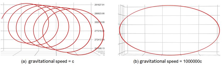
Preprints (www.preprints.org) | NOT PEER-REVIEWED | Posted: 4 January 2022           doi:10.20944/preprints202109.0379.v9

                 sound waves in the water, the speed will be much greater than that of water waves. So
                 the speed of the water waves we observe cannot represent that of sound waves in the
                 water. Will gravitational waves be like this?
                     General relativity (GR), it’s view on the speed of gravity is different from that of
                 Newton and Laplace. GR also believes that the speed of gravity is equal to the speed
                 of light, but until now, scientists have been unable to prove this view. But we know if
                 the gravitational field has a finite speed, there will be a general Doppler effect between
                 the gravitational field and the object. To determine the speed of the gravitational field,
                 we assume the speed of the gravitational field is equal to the speed of light. For the
                 convenience of analysis, we use X to represent the speed of the gravitational field. If
                 the planetary motions of the solar system calculated under this hypothesis are consis-
                 tent with astronomical observations, the correctness of this hypothesis can be proved,
                 otherwise it is proved that the speed of the gravitational field is not equal to that of
                 light.
                     Since we need to analyze the speed of gravity, so we must first figure out what is the
                 relationship between gravity and velocity?

                 2 Derivation of the Relationship between Gravity and Velocity based
                   on Newton’s Gravity Equation
                 In a very short time slice dt, we can assume that m is stationary and the gravity received
                 is constant. We can then accumulate the impulse generated by the gravity on each
                 time slice and find the average relating to the entire time period to obtain effective
                 constant gravitation and determine the relationship between the equivalent gravitation
                 and velocity.
                     Consider the influence of velocity on gravity when the moving velocity of object m
                 relative to M is not 0.

                                                 Figure 1: Gravity model

                     As shown in Figure 1, there are two objects with masses M and m, the distance
                 between them is r, m has a moving velocity relative to M , the speed is v and the
                                                                                                     G0 M m
                 direction of the velocity is depicted by the straight line connecting them. F (t) = (r+vt)2

                 represents the gravity on m at time t. The Newtonian equation of gravity is used here.
                 In any small time dt, m can be regarded as stationary. An accumulation of the impulse

                                                             2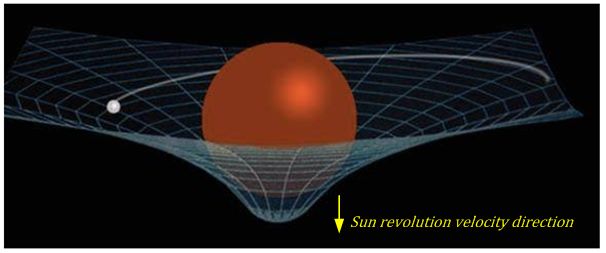
Preprints (www.preprints.org) | NOT PEER-REVIEWED | Posted: 4 January 2022                                               doi:10.20944/preprints202109.0379.v9

                 dp is obtained by multiplying the gravity and time in these small time slices. Then, the
                 sum of the gravitational impulse received by m within a certain period can be obtained.
                 Supposing that the gravitational impulse obtained by m is p after time T has passed,
                 the gravity is integrated into the time domain:
                                   ZT                       ZT                                              ZT
                                                                  G0 M m          G0 M m                              1
                           p=           F (t) × dt =                       × dt =        ×                                   × dt,          (1)
                                                                 (r + vt)2          r2                           (1 + vt/r)2
                                   0                        0                                               0

                      G0 M m        −r/v T
                 p=     r2
                               ×   1+vt/r |0 ,

                      G0 M m         T
                 p=     r2
                               ×   1+vT /r .
                    For an object m with a speed of v, the accumulated impulse p during time T can be
                 expressed by an equivalent constant force multiplied by time T . For the convenience of
                 description, we use F (v) to express this equivalent force.
                                          G0 M m                 vT
                    F (v) = p/T =           r2
                                                 /(1        +     r ).
                     There is an inverse proportional relationship between the equivalent gravitational
                 force and the speed v. The larger the v, the smaller the F (v); the smaller the v, the
                 larger the F (v). When v = 0, it is Newtonian gravity. When v tends to infinity, F (v) =
                 0. The Newtonian gravitational equation is based on the premise that the gravitational
                 field speed is infinite. Now, we may assume that the gravitational field has a finite speed
                 X, therefore, the Newtonian gravitational equation is no longer applicable and need to
                 be modified.
                     Let us continue to think about the difference in the average gravitational force re-
                 ceived by two objects at different speeds during time T ? Assuming that two objects
                 have different velocities, v1 = v0 − δv, v2 = v0 + δv, their average gravity:

                                                     G0 M m                  (v0 −δv)T
                    F (v1 ) = F (v0 − δv) =            r2
                                                            /           1+        r           .

                                                     G0 M m                  (v0 +δv)T
                    F (v2 ) = F (v0 + δv) =            r2
                                                            /           1+        r           .

                                               G0 M m            r                    r
                    F (v1 ) − F (v2 ) =          r2         r+(v0 −δv)T      −   r+(v0 +δv)T          .

                                               G0 M m             2rδvT
                    F (v1 ) − F (v2 ) =          r2         (r+v0 T )2 −(δvT )2
                                                                                      .

                                                                                                          G0 M m       2δvT
                    When T is infinitesimal close to 0, F (v1 ) − F (v2 ) =                                 r2           r        .
                                         T
                    Assume K =           r , δv   = v1 − v2 , so the following formula is obtained:
                    F (v1 ) − F (v2 ) = G0rM2 m (Kδv), we can see that there is a linear relationship between
                 average gravity and velocity, when T is infinitesimal close to 0, the average gravity is
                 the instantaneous gravity.
                     However, we also know that if there is relative velocity between any two objects, there
                 will be a general Doppler effect between them. According to this general Doppler effect

                                                                                  3
Preprints (www.preprints.org) | NOT PEER-REVIEWED | Posted: 4 January 2022 doi:10.20944/preprints202109.0379.v9
between the object and the gravitational field, two Doppler effect boundary conditions
are introduced:
1. When an object’s velocity relative to the source of gravity is 0, it is Newtonian
gravity.
2. When an object’s velocity relative to the gravitational field is 0, the gravitational
force no longer acts on the object.
As shown in the Figure 2, according to the general Doppler effect (chase effect), using
boundary conditions F (0) = G0rM2 m and F (X) = 0, it can be easily calculated:
F (X)−F (0) X−v G0 M m X−v
F (v) = F (0) + v × X = F (0) × X = r2
× X .
Figure 2: Linear relationship between gravity and velocity
From the above analysis, the formula of universal gravitation with parameter v is as
follows:
G0 M m X −v
F (v) = 2
× f (v), f (v) = . (2)
r X
If it is necessary to preserve the form of Newton’s gravity equation, we may write it
as follows:
Mm X −v
F (v) = G(v) × 2
, G(v) = G0 × . (3)
r X
That is, the gravitational constant becomes a function of v, G(v). Thus, we may
understand that when the gravitational field has a different speed relative to m, the
gravitational constant is also different. Next, we apply the new gravitational equation
to the planetary orbit calculation to determine whether it is consistent with actual
observations.
4Preprints (www.preprints.org) | NOT PEER-REVIEWED | Posted: 4 January 2022 doi:10.20944/preprints202109.0379.v9
3 Calculation of the Influence of the New Gravitational Equation on
Earth’s Orbit
From the above derivation, we get the gravity formula with v as a parameter:
G0 M m X−v
F (v) = r2
× X .
Considering that the velocity direction of the object m may have an angle with the
gravitational field, we define vr as the component of the speed in the direction of the
gravitational field and then obtain a general formula:
G0 M m X−vr
F (vr ) = r2
× X .
The equation shows that when an object has a velocity component in the direction of
the gravitational field, that is, there is a movement effect in the same direction between
the gravitational field and the object, the gravitational force received decreases. When
the object has a velocity component that is opposite to the direction of the gravitational
field, that is, the two have the effect of moving towards each other, the gravitational
force received increases. This leads us to thus consider what impact, under this general
Doppler effect, it may have on the planet’s orbit. Can planets maintain the conservation
of mechanical energy in their orbits?
Figure 3: The velocity component of the planet’s gravitational field direction
As shown in Figure 3, under the new gravitational equation, as the planetary velocity
has the same direction component vr in the direction of the gravitational field in orbits
A and B, the gravity decreases. Therefore, the planet gains extra force in the direction
of the gravitational field. This force travels in the same direction as vr . According to the
power calculation formula P = F × vr > 0, the planetary mechanical energy increases.
Regarding regions C and D, as the planetary velocity has a reverse component vr in
the direction of the gravitational field, the gravitational force increases. Therefore, the
5Preprints (www.preprints.org) | NOT PEER-REVIEWED | Posted: 4 January 2022 doi:10.20944/preprints202109.0379.v9
extra force gained by the planet moves in the opposite direction of the gravitational field.
This force is in the same direction as vr . According to the power calculation formula
P = F × vr > 0, the planetary mechanical energy increases.
Therefore, under the new gravitational equation, the mechanical energy of the planet
in the entire orbit continues to increase and the mechanical energy becomes larger and
larger. This would cause the planet to gradually move away from the Sun and eventually
the solar system. Taking Earth as an example, using the new gravitational equation,
after how many revolution cycles would Earth begin to move away from the solar system?
Below we include our theoretical analysis and calculations.
3.1 Introduction of Polar Coordinates
Let the Sun, mass M , lie at the origin. Consider a planet, mass m, in orbit around the
Sun. Let the planetary orbit lie in the x − y plane. Let r(t) be the planet’s position
vector with respect to the Sun. The planet’s equation of motion is
G0 M m X − v
mr̈ = − × × er , (4)
r2 X
where er = r/r and vr = er .ṙ.Let r = |r|and θ = tan−1 (y/x) be plane polar coordinates.
The radial and tangential components of (4) are
G0 M ṙ
r̈ − rθ̇2 = − 1 − (5)
r2 X
rθ̈ + 2ṙθ̇ = 0 (6)
(6) can be integrated to give
r2 θ̇ = h (7)
where h is the conserved angular momentum per unit mass. (5),(7) can be combined to
give
h2 G0 M ṙ
r̈ − 3
=− 2 1− (8)
r r X
3.2 Energy Conservation
Multiply (8) by ṙ. We obtain
d ṙ2 h2 G0 M G0 M ṙ2
+ 2− = (9)
dt 2 2r r r2 X
6Preprints (www.preprints.org) | NOT PEER-REVIEWED | Posted: 4 January 2022 doi:10.20944/preprints202109.0379.v9
or
d G0 M ṙ2
= ≥0 (10)
dt r2 X
where
1 G0 M
= (ṙ2 + r2 θ̇2 ) − (11)
2 r
is the energy per unit mass. (10) demonstrates that the Doppler shift correction to the
law of force causes the system to cease conserving energy. The orbital energy grows
without limit. This means that the planet will eventually escape the Sun’s gravitational
pull (when its orbital energy becomes positive).
3.3 Solution of Equations of Motion
Let 1/r = u[θ(t)]. It follows that
du
ṙ = −h , (12)
dθ
d2 u
r̈ = −u2 h2 , (13)
dθ2
thus, Eq. (8) becomes
d2 u du G0 M
2
−γ +u= , (14)
dθ dθ h2
where
G0 M
γ= , (15)
hX
is a small dimensionless constant. To first order in γ, an appropriate solution of (14) is
G0 M
u≈ (1 + e exp(γθ) cos θ), (16)
h2
where e is the initial eccentricity of the orbit. Thus
rc
r(θ) = , (17)
1 + e exp(γθ) cos θ
7Preprints (www.preprints.org) | NOT PEER-REVIEWED | Posted: 4 January 2022 doi:10.20944/preprints202109.0379.v9
where
h2
rc = . (18)
G0 M
It can be observed that the orbital eccentricity grows without limit as the planet
orbits the Sun. Eventually, when the eccentricity becomes unity, the planet will escape
the Sun.
3.4 Estimation of Escape Time
The planet escapes when its orbital eccentricity becomes unity. The number of orbital
revolutions, n, required for this to happen is
e exp(γn2π) = 1, (19)
1
where e is the initial eccentricity. Thus, n = 2πγ ln( 1e ),
2πa
γ= 1 , (20)
T X(1 − e2 ) 2
where a is the initial orbital major radius and T is the initial period. Hence,
1
T X(1 − e2 ) 2 ln( 1e )
n= . (21)
4π 2 a
For Earth, T = 3.156 × 10⁷ s, X = c = 2.998 × 10⁸ m/s, a = 1.496 × 10¹¹ m, and
e = 0.0167. Hence, Earth would escape from the Sun’s gravitational influence after
1
1
(3.156 × 10⁷ )(2.998 × 10⁸ )(1 − 0.01672 ) 2 ln( 0.0167 )
n= 2 11
≈ 6.6 × 10³ , (22)
4π (1.496 × 10 )
revolutions. If each revolution takes approximately 1 year, then the escape time is a few
thousand years. However, the age of the solar system is 4.6 × 10⁹ years. The escape time
is smaller than this by a factor of approximately one million. Therefore, the speed of
gravitational waves cannot represent the speed of the gravitational field. From equation
(22), the speed of a gravitational field X must be much greater than the speed of light
c[10] ; this is more in line with Newton’s argument that the force of gravity acts at a
distance.
We may consider the following analogy: we use a rope to pull a kite. When we shake
it hard, the rope will fluctuate and pass to the kite at a certain wave speed, however,
8Preprints (www.preprints.org) | NOT PEER-REVIEWED | Posted: 4 January 2022 doi:10.20944/preprints202109.0379.v9
when we loosen the rope, the kite instantly loses control. It is inappropriate to use the
wave speed of the rope to represent the speed of the force of the rope on the kite. With
this considered, how do gravitational waves affect gravity? Since the revolution speed of
the Sun will cause gravitational waves, how are gravitational waves distributed around
the Sun?
4 The Influence of Gravitational Waves Produced by the Sun on the
Surrounding Gravity
Gravitational waves caused by the movement of the Sun are akin to water waves caused
by ships. For the convenience of explanation, we have turned the three-dimensional
space problem into a two-dimensional problem. The gravitational influence caused by
gravitational waves is different in the direction of the Sun’s velocity and the vertical
direction, as shown in Figure 4.
Figure 4: The gravitational wave model generated by the Sun’s movement.
Assuming that, without considering the general Doppler effect, the ratio of the grav-
itational increase caused by gravitational waves to Newtonian gravitation is rw , we
introduce a gravitational wave influence factor of fw . Figure 4 shows that, due to the
general Doppler effect of gravitational waves, the energy of gravitational waves is largest
in the direction of the Sun’s velocity and the impact on gravity is the greatest. The
planet’s orbital surface is perpendicular to the direction of the Sun’s velocity and the
gravitational wave is relatively small.
9Preprints (www.preprints.org) | NOT PEER-REVIEWED | Posted: 4 January 2022 doi:10.20944/preprints202109.0379.v9
Figure 5: The solar gravitational wave calculation model
4.1 Calculation of the Influence Factor of Gravitational Waves in the Direction of the
Sun’s Velocity
We know that the revolution speed of the Sun is vs . Assuming that the Sun moves from
position O to position O0 after time T , the gravitational waves generated in the direction
of the Sun’s velocity during this period are all located between O0 B. According to the
general Doppler effect of gravitational waves, the influence factor of gravitational waves
in this direction is as below:
c + vs
fw = > 1.0. (23)
c
4.2 Calculation of the Influence Factor of Gravitational Waves in the Vertical Direc-
tion of the Sun’s Velocity
The gravitational waves in the direction perpendicular to the Sun’s velocity are located
between O0 A; it is only necessary to calculate the ratio between O0 B and O0 A to deter-
mine the gravitational wave density relationship in the two directions.
O0 B = cT − vs T, (24)
10Preprints (www.preprints.org) | NOT PEER-REVIEWED | Posted: 4 January 2022 doi:10.20944/preprints202109.0379.v9
1
O0 A = [(cT )2 − (vs T )2 ] 2 , (25)
thus:
1 1
c + vs c − vs 2 c2 − vs2 2
fw ≈ × = . (26)
c c + vs c2
Substituting the solar revolution speed vs = 240 × 103 m/s and the gravitational
0 1
c−vs 2
wave speed c = 2.998 × 10⁸ m/s, we get O B
O0 A = ( c+vs ) ≈ 0.9992. Figure 4 shows that
the density of gravitational waves in the vertical direction is smaller than that in the
direction of the Sun’s velocity. The density of gravitational waves gradually decreases
from the direction of the Sun’s velocity to the vertical direction. If the gravitational wave
density is equivalent to the level of the depression in the plane, then this gravitational
wave density model is somewhat similar to the space-time depression model described
by general relativity (GR). As shown in the Figure 6, the gravitational wave density
presents a non-uniform distribution; gravitational waves have the highest density in the
direction of the sun’s velocity (bottom of Figure 6), and gradually decrease upwards.
Figure 6: Gravitational wave density model
4.3 Calculation of the Influence Factor of Gravitational Waves on the Planetary Or-
bital Surface
We know that the planet’s orbital plane is approximately perpendicular to the direction
of the Sun’s motion; thus, the red line in Figure 5 represents the ideal orbital plane of the
planet (completely perpendicular to the direction of the sun’s velocity). According to
formula (26), we can calculate the influence factor of gravitational waves on the orbital
surface and thus determine that this value will be less than 1.0.
11Preprints (www.preprints.org) | NOT PEER-REVIEWED | Posted: 4 January 2022 doi:10.20944/preprints202109.0379.v9
4.4 Calculation of the Influence Factor of Gravitational Waves on the Reverse of the
Sun’s Velocity
Behind the vertical plane (to the left of the red line in Figure 5), shows that the density
of the gravitational waves will continue to decrease and reach a minimum in the opposite
0B c−vs
direction of the Sun’s velocity. At this time O
O0 C = c+vs , the gravitational wave influence
factor is as below:
c + vs c − vs c − vs
fw ≈ × = . (27)
c c + vs c
Substituting vs = c into (26) and (27), it can be determined that when the speed of
the Sun reaches c, the orbital surface of the planet perpendicular to the Sun’s velocity
(the position of the red line) and the position behind it (the left side of the red line) is
no longer affected by gravitational waves.
4.5 Calculation of the Influence Factor of Gravitational Waves at any Position
As shown in Figure 5, assuming that the angle between O0 D and the red line is θ (with
D at any position), then
π
OD2 = O0 D2 + OO02 − 2O0 D × OO0 cos( − θ), (28)
2
we get:
1
2OO0 cos( π −θ)+[4(OO0 cos( π −θ))2 −4(OO02 −OD2 )] 2
O0 D = 2
2
2
,
then,
O0 B 2O0 B
0
= 1 , (29)
OD 2OO0 cos( π2 − θ) + [4(OO0 cos( π2 − θ))2 − 4(OO02 − OD2 )] 2
thus:
c + v
s c − vs
fw ≈ × 1 . (30)
c vs cos( π2 − θ) + [(vs cos( π2 − θ))2 − (vs2 − c2 )] 2
4.6 The Influence of Gravitational Waves on Gravity
Assuming that the gravitational force of an object under the influence of gravitational
waves is Fw , Fw can be regarded as two parts:
G0 M m
Part 1: Newtonian gravity F = r2
.
Part 2: The gravity contributed by the gravitational wave rw fw F , where rw is the
ratio of the gravitational increase caused by gravitational waves to Newtonian gravita-
tion.
12Preprints (www.preprints.org) | NOT PEER-REVIEWED | Posted: 4 January 2022 doi:10.20944/preprints202109.0379.v9
Thus, we get:
Fw = F + rw × fw × F. (31)
Let us take the orbital position as an example to illustrate the calculation of gravity
under the influence of gravitational waves:
c2 − v 2 1
s 2
Fw = F + rw × fw × F = F × 1 + rw × . (32)
c2
As there is also a general Doppler effect between planets and gravitational waves,
it is also necessary to consider the influence of this factor. Assuming that the speed of
the planet is vp and the speed of the planet in the direction of the gravitational wave is
c−v
vpw , then the chase factor c pw between the planet and the gravitational wave can be
obtained and this factor is put into (32) to get:
c2 − v 2 1 c − vpw
s 2
Fw = F × 1 + rw × × , (33)
c2 c
substituting F , we get:
G0 M m c2 − v 2 1 c − vpw
s 2
Fw = × 1 + rw × × , (34)
r2 c2 c
here rw ≈ 0.00058; this value was derived from a program simulation.
In the same way, the gravity of other positions can be calculated. We write the
gravity equation of any position:
!!
G0 M m c + vs c − vs c − vpw
Fw = 2
× 1+rw × × 1 ×
r c π π
vs cos( 2 − θ) + [(vs cos( 2 − θ))2 − (vs2 − c2 )] 2 c
(35)
4.7 Gravitational Waves Caused by the Rotation of the Sun
The Sun’s rotation can also cause gravitational waves, however, the Sun’s revolution
speed of 240 km/s is much greater than its rotation speed of 2 km/s. As such, this
physical model does not consider the influence of gravitational waves caused by rotation.
To obtain more precise calculations, we must consider this factor.
13Preprints (www.preprints.org) | NOT PEER-REVIEWED | Posted: 4 January 2022 doi:10.20944/preprints202109.0379.v9
5 Analysis of the Influence of Gravitational Waves on Planetary Orbits
If the planet’s orbital surface is not completely perpendicular to the velocity of the Sun
and the orbit is split over both sides of the red line, then the impact of gravitational
waves on planets is also irregular, which affects the orbit and contributes part of the
force to planetary precession[9] . The closer the planet’s orbit is to the Sun, the greater
the gravitational wave density gradient and the more obvious the effect of precession;
the farther the distance, the less obvious. Similarly, the larger the angle between the real
planetary orbit surface and the red line in Figure 5, the more obvious the precession.
In 1915, Albert Einstein published in [1915, p. 839][9] a formula for the relativistic
perihelion shift, for one period, of
a2
ε = 24π 3 , (36)
T 2 c2 (1 − e2 )
where according to contemporary data T is the orbital period of planet, e is the
eccentricity of its elliptical orbit, a is the length of its corresponding semimajor axis,
and c is the speed of light in vacuum.
τ 180
δ ϕ̇ = ε 3600”, (37)
T π
here τ = 3155814954 s is the number of seconds in one century. We can also use a
simplified calculation formula of GR.
0.0383
δ ϕ̇ ' . (38)
RT
From the formulas (37) and (38), GR does not consider the angle between the real
planet’s orbital plane and the Sun’s vertical plane (the red line in Figure 5), and the
eccentricity of the orbit is not the main factor either, when calculating the planetary
precession. However, we must consider them as the main factors in the data calculated
by formula (35). These may be the biggest differences between the two. Below, we
substitute the R and T values of each planet (see Figure 7) for GR calculation.
14Preprints (www.preprints.org) | NOT PEER-REVIEWED | Posted: 4 January 2022 doi:10.20944/preprints202109.0379.v9
Figure 7: Data for the major planets in the solar system, giving the planetary mass
relative to that of the Sun, the orbital period in years, and the mean orbital radius
relative to that of Earth.
The calculated precession data of each planet per century is as follows:
Mercury 41.06”
Venus 8.6”
Earth 3.83”
Mars 1.34”
Jupiter 0.062”
Saturn 0.0136”
Uranus 0.00238”
But we must note that when GR calculates the planet precession deviation, it ignores
the rotation of the Sun around the center of mass of the solar system and the influence of
planets on the Sun’s gravity. GR constructs an idealized 1-body model. 1-body means
there is only one planet in the solar system.
In order to maintain consistency with GR, we also made the same omission, con-
structed the same 1-body ideal model, and calculated the precession of each planet. If
we want the calculated results to be closer to the real 1-body system, we cannot ignore
the influence of the planets on the Sun, nor the rotation of the Sun around the center
of mass of the 1-body system. We have made a clear comparison of all calculated data
in the table below. We can see that the gravitational model constructed according to
formula (35), without considering the influence of gravitational waves (that is, classical
Newtonian mechanics), the planet precession is zero. And considering the influence of
gravitational waves, the planet precession in the 1-body system is relatively close to the
results calculated by GR. We did not find the data of GR in the real 1-body system, but
15Preprints (www.preprints.org) | NOT PEER-REVIEWED | Posted: 4 January 2022 doi:10.20944/preprints202109.0379.v9
according to the analysis of GR, the changes in the data are very small. The data we
calculated using the gravitational wave theory also reflected this.(The precession data
in the paper are all calculated after the perihelion is projected onto the x-y plane.)
Figure 8: 1-body planetary orbit precession per century
Except for Venus’s precession data of 169” vs 8.6”, the data of other planets are
relatively close to GR.
Let us examine the characteristics of Venus: Venus’s eccentricity is abnormally low
(e = 0.0068), which makes its perihelion extremely sensitive to small disturbances. How-
ever, the angle between its orbit and the vertical plane of the Sun is very large (3.39°);
thus, we have reason to believe that gravitational waves will have a significant influence
on the orbital precession of Venus.
Why is the data of Venus (169” vs 8.6”) so different? From formulas (37) and (38),
it can be determined that GR does not take eccentricity as the main factor and does
not consider the angle between the orbital surface and the vertical surface of the Sun.
Under different eccentricities and angles, the precession data calculated by GR remains
the same. This may be the reason for the large difference between the two.
We know that the famous Mercury Precession 43” comes from the comparison be-
tween the calculated data of the planetary orbit of the solar system by Newton’s classical
mechanics and the astronomical observation data. This requires the calculation of all the
planets in the solar system, the gravitational force between the planets and the Sun, the
gravitational force between the planets, and the rotation of the Sun around the center
of mass of the solar system to construct a real N-body system. Then it is necessary
to calculate the planet precession data under and without the influence of gravitational
waves. Since GR does not provide planetary precession data under the N-body system,
it cannot be compared with GR. We can see that the data under the action of gravita-
tional waves are different. For Mercury, the difference between the two is close to the
data under the 1-body model 43”. (The initial coordinates (x, y, z) and initial velocity
(vx, vy, vz) datas of the planets and the Sun used in this paper are all from NASA’s
16Preprints (www.preprints.org) | NOT PEER-REVIEWED | Posted: 4 January 2022 doi:10.20944/preprints202109.0379.v9
Horizons System https://ssd.jpl.nasa.gov/horizons/.)
Figure 9: N-Body planetary orbit precession per century
In addition, we must emphasize that the common period of the orbits of the eight
planets in the solar system is very huge, so it is difficult for us to obtain the orbital
precession laws of planets with very small eccentricities through short-term calculations.
Through 200 years of astronomical observations, we also cannot get the periodic pre-
cession laws of all planets, and it takes longer to observe. But for Mercury and Mars,
their eccentricity is relatively large, and we can easily get their approximate general laws
through calculations or astronomical observations.
Since the orbital data is obtained through integration in the time domain, the av-
eraged precession data obtained in each orbital period has a certain range of variation.
The data in the following table is a piece of data randomly selected after 4000 Mer-
cury cycles. We can see that the precession data is changing. As time increases, this
change will be further statistically averaged and gradually reduced. We can see that the
influence of gravitational waves on Mercury’s precession also changes around 39”.
17Preprints (www.preprints.org) | NOT PEER-REVIEWED | Posted: 4 January 2022 doi:10.20944/preprints202109.0379.v9
Figure 10: Mercury precession data per century
In addition to causing planetary precession, gravitational waves also cause planets
to move away from the Sun. We know there is also a general Doppler effect between the
planet’s revolution velocity and the gravitational waves caused by the Sun. The previous
3.2 ”Energy Conservation” has analyzed the influence of the general Doppler effect on
orbital energy. Gravitational waves also cause the planetary orbital mechanical energy
to continue to increase; this causes planets to gradually move away from the Sun.
We applied this gravitational theory to calculate the detailed planetary orbit data
(x, y, z), and used 3D technology to draw these data, as shown in Figure 11 and Figure
12, we can clearly observe the orbits of the Sun and planets around the center of mass of
the solar system. As shown in Figure 13, when we magnify the z-axis data by 10 times,
we can clearly see the angle between the planetary orbital surfaces.
18Preprints (www.preprints.org) | NOT PEER-REVIEWED | Posted: 4 January 2022 doi:10.20944/preprints202109.0379.v9
Figure 11: Sun rotation orbit
Figure 12: Planetary orbit
19Preprints (www.preprints.org) | NOT PEER-REVIEWED | Posted: 4 January 2022 doi:10.20944/preprints202109.0379.v9
Figure 13: The angle between the planetary orbital surfaces
GR believes that the speed of gravity is equal to the speed of light. If this is true,
then the orbits of the planets and the Sun in the solar system should at least remain
stable. We have added the gravitational speed parameter to the program, which can be
set arbitrarily, such as equal to 0.1c, equal to c, equal to 100c, and so on. Especially
in a binary star system (1-body), when the gravitational speed parameter is set to c,
we can clearly observe that the orbits of the planets and the Sun will no longer be
stable. As shown in Figure 14(a), the solar orbit will spiral in a certain direction. By
simulating different gravitational speeds, we have come to the conclusion that the lower
the gravitational speed, the more unstable the solar system. The theoretical basis of GR
is that the speed of gravity is equal to the speed of light, but the accuracy of the orbit
simulation is not reflected. Even if the space-time is curved, the orbit will not remain
stable.
Figure 14: The orbit of the Sun at different gravitational speeds.
As shown in Figure 15, we have built a very simple Sun-Earth model. If the grav-
itational speed is equal to the speed of light, the gravitational force of the Sun will be
delayed for 8 minutes, then the gravitational force of the Sun on the Earth will come
from S1 instead of the true position S0, so there will be a component F 1 that is opposite
to the orbital velocity of the Sun, under the action of F 1 , The Earth will move to the
left, as shown in Figure 15(a). Finally, the Earth will follow S1, as shown in Figure
20Preprints (www.preprints.org) | NOT PEER-REVIEWED | Posted: 4 January 2022 doi:10.20944/preprints202109.0379.v9
15(b), which is inconsistent with the real solar system. Tom van Flandern’s paper[11]
also elaborated that the gravitational speed is much greater than the speed of light.
Figure 15: Sun-Earth model at the gravitational speed equal to the speed of light
6 Einstein–Infeld–Hoffmann Equations
The Einstein–Infeld–Hoffmann equations[12] of motion, jointly derived by Albert Ein-
stein, Leopold Infeld and Banesh Hoffmann, are the differential equations of motion
describing the approximate dynamics of a system of point-like masses due to their mu-
tual gravitational interactions, including general relativistic effects. It uses a first-order
post-Newtonian expansion and thus is valid in the limit where the velocities of the bod-
ies are small compared to the speed of light and where the gravitational fields affecting
them are correspondingly weak. Given a system of N bodies, labelled by indices A = 1,
..., N, the barycentric acceleration vector of body A is given by:
21Preprints (www.preprints.org) | NOT PEER-REVIEWED | Posted: 4 January 2022 doi:10.20944/preprints202109.0379.v9
Figure 16: Einstein–Infeld–Hoffmann equations
The coordinates used here are harmonic. The first term on the right hand side is the
Newtonian gravitational acceleration at A; in the limit as c → ∞, one recovers Newton’s
law of motion. It seems that this equation is perfect.
The Einstein-Infeld-Hoffmann equations are a weak field linearized version of GR that
are appropriate when the curvature of spacetime is not too severe. This is certainly the
case in the Solar System. The full nonlinear version of GR is only needed in situations
in which the curvature of spacetime is severe, such as in the immediate vicinity of a
black hole. The speed of gravitational effects in the Einstein-Infeld-Hoffmann equations
is the speed of light, which is why c appears in these equations. However, the corrections
to planetary orbits, relative to Newtonian dynamics, predicted by the Einstein-Infeld-
Hoffmann equations are very minor.
We can simplify this equation. We only consider the binary star system. There are
only two objects A and B. When the mass of B is much greater than the mass of A, vB
22Preprints (www.preprints.org) | NOT PEER-REVIEWED | Posted: 4 January 2022 doi:10.20944/preprints202109.0379.v9
is approximately equal to 0, so the equation is simplified to an equation with only A.
When the speed of the gravitational field is much greater than c, then it is Newtonian
gravitation. c → ∞, one recovers Newton’s law of motion, there seems to be no problem.
When the speed of the gravitational field is much smaller than c, then the result of
this equation has almost nothing to do with Newtonian gravity. c → 0, force on A and
B will both be very huge, which is very illogical!
The equations in question are the first few terms on an expansion, so obviously the
equations do not give a sensible answer when c goes to zero because the expansion breaks
down. Therefore, I believe that the equation is a mathematical model established under
the assumption that the gravitational speed is equal to c to describe the planetary orbit
under N-BODY. But it does not really describe the physical properties of gravity.
Einstein thought Gravitation is bending of space-time. everything moving with con-
stant speed either it be light or anything else always follows geodesic. Then I want to
ask a question: If the light is aimed at the center of the planet, what is the geodesic at
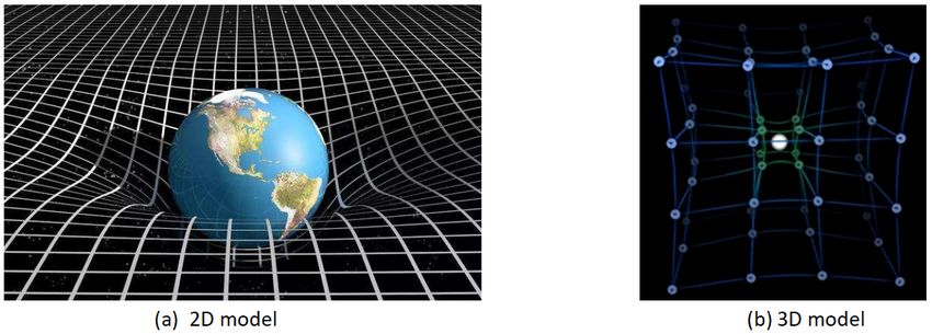
this time? Will the light be bent? If our Earth also bends the surrounding space-time,
then looking at the 2D space-time bending model, as shown in Figure 17(a), the light
will never have a chance to reach the earth, and the light will only travel along the
bent space-time, from the edge of the earth, go through. Obviously this 2D space-time
bending model is incorrect, so will the 3D space-time bending model be correct? As
shown in Figure 17(b), it can be seen that the surrounding space is recessed toward the
center. The more severe the bending, the greater the impact of mass on space-time.
It seems that the 3D model is closer to the truth. But if we express the magnitude of
Newtonian gravitation at different positions in space as the distance from the source of
gravity, then the final 3D model of Newtonian gravitation is almost the same as the 3D
model of GR’s space-time bending. It seems that Newton can also claim that univer-
sal gravitation bends space-time, but the fact is that it is only a mathematical model
that uses distance to express the magnitude of gravitation. In this mathematical model,
there are only coordinates of the direction and the magnitude of gravity, and no space
coordinates (x, y, z), space-time have never been bent. But Einstein obviously confuses
these concepts. Not only does he use the degree of bending to express the magnitude
of gravity, but also continues to retain the spatial coordinates (x, y, z). GR is a wrong
theory of gravity, which doomed the Einstein-Infield-Hoffman equation to be wrong.
23Preprints (www.preprints.org) | NOT PEER-REVIEWED | Posted: 4 January 2022 doi:10.20944/preprints202109.0379.v9
Figure 17: bending of space-time
7 Conclusion
The discovery of gravitational waves provides a new way for us to understand the uni-
verse, however, the speed of gravitational waves does not represent the speed of gravita-
tional fields. The speed of action of gravitational fields is much greater than the speed
of gravitational waves. As stated by Newton: Gravity is an action-at-a-distance force.
Gravitational waves caused by the revolution of the Sun affect the orbits of planets and
provide some planetary precession data. The general Doppler effect of gravitational
waves also causes the planetary orbital mechanical energy to continue to increase slowly
until the planet escapes from the solar system. Gravitational waves exist; the grav-
itational model under the influence of gravitational waves that we constructed was a
physical model. Through the calculation of planetary orbital precession, the correctness
of the gravity equation under the action of gravitational waves is verified, indicating
that the gravitational physical model has research value. From Newton to Pierre-Simon
Laplace have realized that the speed of gravity on objects is very huge. But this view is
inconsistent with GR. From our analysis, GR is a wrong theory of gravity. The Newto-
nian model of universal gravitation under the action of gravitational waves is the correct
way for humans to study the universe.
Finally, we also ask the following questions:
Is the acceleration of planetary orbits caused by the gravitational wave general
Doppler effect related to the accelerated expansion of the universe?
Is there an association between the action-at-a-distance of the gravitational field and
that in quantum mechanics?
24Preprints (www.preprints.org) | NOT PEER-REVIEWED | Posted: 4 January 2022 doi:10.20944/preprints202109.0379.v9
References:
[1] Fritz Rohrlich (25 August 1989). From Paradox to Reality: Our Basic Concepts of
the Physical World. Cambridge University Press. pp. 28–. ISBN 978-0-521-37605-1.
[2] Newtonian Gravity http://farside.ph.utexas.edu/teaching/336k/Newtonhtml/node35.html
[3] ”2018 CODATA Value: Newtonian constant of gravitation”. The NIST Reference on
Constants, Units, and Uncertainty. NIST. 20 May 2019. Retrieved 2019-05-20.
[4] ”Doppler Shift”. astro.ucla.edu.
[5] The Detection of Gravitational Waves using LIGO, B. Barish Archived 2016-03-03
at the Wayback Machine
[6] Abbott, R.; et al. (29 June 2021). ”Observation of Gravitational Waves from Two
Neutron Star–Black Hole Coalescences”. The Astrophysical Journal Letters. 915 (1).
doi:10.3847/2041-8213/ac082e. Retrieved 29 June 2021.
[7] Barry C. Barish, Caltech. The Detection of Gravitational Waves. Video from CERN
Academic Training Lectures, 1996
[8] ”Physics: Fundamental Forces and the Synthesis of Theory — Encyclopedia.com”.
www.encyclopedia.com.
[9] Einstein A., 1915, Erkl¨arung der Perihelbewegung des Merkur aus der allgemeinen
Relativit¨atstheorie. K¨oniglich-Preußische Akad. Wiss. Berlin, pp. 831–839. English
translation “Explanation of the perihelion motion of Mercury from general relativity
theory” by R. A. Rydin with comments by A. A. Vankov, 1–34.
[10] Michal Krizek. Numerical experience with the finite speed of gravitational interac-
tion. November 1999 Mathematics and Computers in Simulation 50(1-4):237-245 Follow
journal, DOI: 10.1016/S0378-4754(99)00085-3
[11] The Speed of Gravity – What the Experiments Say December 1998Physics Letters
A 250(s 1–3) DOI: 10.1016/S0375-9601(98)00650-1
[12] Einstein, A.; Infeld, L.; Hoffmann, B. (1938). ”The Gravitational Equations and
the Problem of Motion”. Annals of Mathematics. Second series. 39 (1): 65–100. Bib-
code:1938AnMat..39...65E. doi:10.2307/1968714. JSTOR 1968714.
25You can also read


