Grid Generator Grid Generator for MIKE 21C - User Guide
←
→
Page content transcription
If your browser does not render page correctly, please read the page content below
Grid Generator

                           Grid Generator for MIKE 21C

                                            User Guide

Powering Water Decisions                       MIKE 2022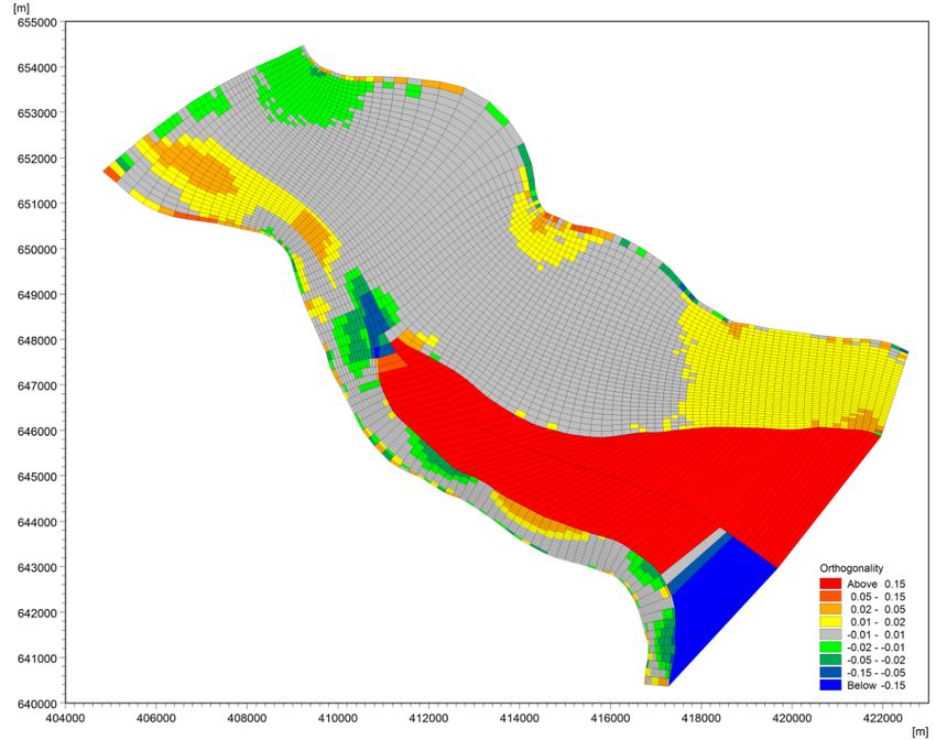
2
PLEASE NOTE

COPYRIGHT                  This document refers to proprietary computer software which is pro-
                           tected by copyright. All rights are reserved. Copying or other repro-
                           duction of this manual or the related programs is prohibited without
                           prior written consent of DHI A/S (hereinafter referred to as “DHI”).
                           For details please refer to your 'DHI Software Licence Agreement'.

LIMITED LIABILITY          The liability of DHI is limited as specified in your DHI Software
                           Licence Agreement:

                           In no event shall DHI or its representatives (agents and suppliers)
                           be liable for any damages whatsoever including, without limitation,
                           special, indirect, incidental or consequential damages or damages
                           for loss of business profits or savings, business interruption, loss of
                           business information or other pecuniary loss arising in connection
                           with the Agreement, e.g. out of Licensee's use of or the inability to
                           use the Software, even if DHI has been advised of the possibility of
                           such damages.

                           This limitation shall apply to claims of personal injury to the extent
                           permitted by law. Some jurisdictions do not allow the exclusion or
                           limitation of liability for consequential, special, indirect, incidental
                           damages and, accordingly, some portions of these limitations may
                           not apply.

                           Notwithstanding the above, DHI's total liability (whether in contract,
                           tort, including negligence, or otherwise) under or in connection with
                           the Agreement shall in aggregate during the term not exceed the
                           lesser of EUR 10.000 or the fees paid by Licensee under the Agree-
                           ment during the 12 months' period previous to the event giving rise
                           to a claim.

                           Licensee acknowledge that the liability limitations and exclusions
                           set out in the Agreement reflect the allocation of risk negotiated and
                           agreed by the parties and that DHI would not enter into the Agree-
                           ment without these limitations and exclusions on its liability. These
                           limitations and exclusions will apply notwithstanding any failure of
                           essential purpose of any limited remedy.

Powering Water Decisions                                                                              3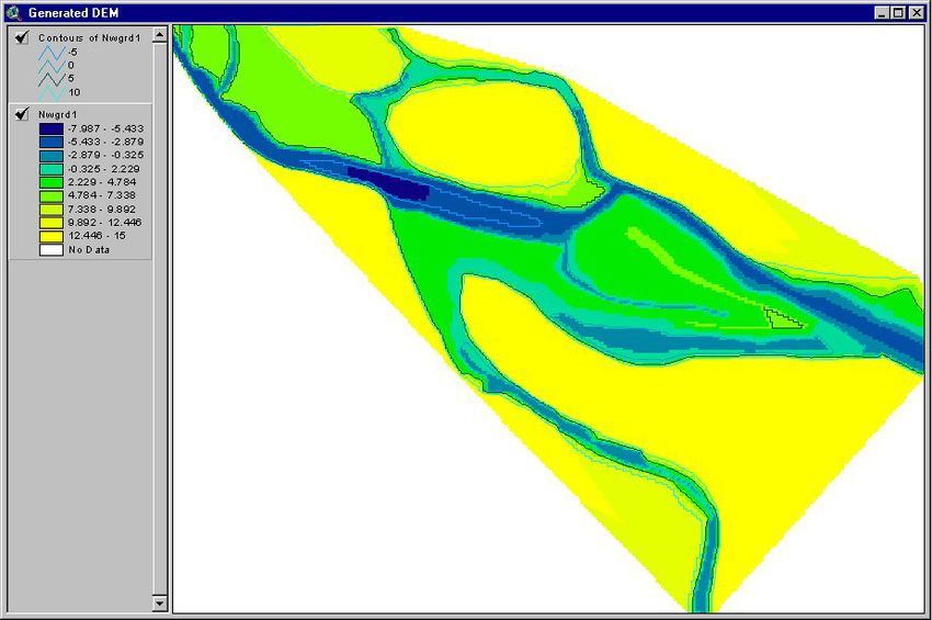
4 MIKE 21C Grid Generator - © DHI A/S
CONTENTS

1     Reference Manual . . . . . . . . . . . . . . . . . . . . . . . . . . . . . . . . . .                                                7
      1.1     Introduction . . . . . . . . . . . . . . . . . .   .   .   .   .   .   .   .   .   .   .   .   .   .   .   .   .   .   .    7
              1.1.1    Start of new application . . . . . . .    .   .   .   .   .   .   .   .   .   .   .   .   .   .   .   .   .   .    9
              1.1.2    Creating a new grid . . . . . . . . .     .   .   .   .   .   .   .   .   .   .   .   .   .   .   .   .   .   .   11
              1.1.3    Modifying a grid . . . . . . . . . . .    .   .   .   .   .   .   .   .   .   .   .   .   .   .   .   .   .   .   12
              1.1.4    Grid orthogonality . . . . . . . . . .    .   .   .   .   .   .   .   .   .   .   .   .   .   .   .   .   .   .   13
              1.1.5    Specifications for grid generator . .     .   .   .   .   .   .   .   .   .   .   .   .   .   .   .   .   .   .   14
      1.2     New Grid . . . . . . . . . . . . . . . . . . .     .   .   .   .   .   .   .   .   .   .   .   .   .   .   .   .   .   .   14
              1.2.1    Specifications . . . . . . . . . . . .    .   .   .   .   .   .   .   .   .   .   .   .   .   .   .   .   .   .   15
              1.2.2    Action buttons . . . . . . . . . . . .    .   .   .   .   .   .   .   .   .   .   .   .   .   .   .   .   .   .   16
      1.3     Merge Grids . . . . . . . . . . . . . . . . .      .   .   .   .   .   .   .   .   .   .   .   .   .   .   .   .   .   .   17
      1.4     Add Grid . . . . . . . . . . . . . . . . . . .     .   .   .   .   .   .   .   .   .   .   .   .   .   .   .   .   .   .   18
      1.5     Grid Operations . . . . . . . . . . . . . . .      .   .   .   .   .   .   .   .   .   .   .   .   .   .   .   .   .   .   19
              1.5.1    Draw grid orientation . . . . . . . .     .   .   .   .   .   .   .   .   .   .   .   .   .   .   .   .   .   .   20
              1.5.2    Edit grid points . . . . . . . . . . .    .   .   .   .   .   .   .   .   .   .   .   .   .   .   .   .   .   .   21
              1.5.3    Select subgrid . . . . . . . . . . . .    .   .   .   .   .   .   .   .   .   .   .   .   .   .   .   .   .   .   21
              1.5.4    Generate border . . . . . . . . . .       .   .   .   .   .   .   .   .   .   .   .   .   .   .   .   .   .   .   22
              1.5.5    Grid update - orthogonalisation . . .     .   .   .   .   .   .   .   .   .   .   .   .   .   .   .   .   .   .   24
              1.5.6    Extract subgrid . . . . . . . . . . .     .   .   .   .   .   .   .   .   .   .   .   .   .   .   .   .   .   .   27
              1.5.7    Resize grid . . . . . . . . . . . . .     .   .   .   .   .   .   .   .   .   .   .   .   .   .   .   .   .   .   28
              1.5.8    Add land border . . . . . . . . . . .     .   .   .   .   .   .   .   .   .   .   .   .   .   .   .   .   .   .   29
              1.5.9    Grid info . . . . . . . . . . . . . . .   .   .   .   .   .   .   .   .   .   .   .   .   .   .   .   .   .   .   29
              1.5.10 Add item . . . . . . . . . . . . . .        .   .   .   .   .   .   .   .   .   .   .   .   .   .   .   .   .   .   30
              1.5.11 Add item from file . . . . . . . . . .      .   .   .   .   .   .   .   .   .   .   .   .   .   .   .   .   .   .   31
              1.5.12 Items . . . . . . . . . . . . . . . .       .   .   .   .   .   .   .   .   .   .   .   .   .   .   .   .   .   .   31
      1.6     Polyline . . . . . . . . . . . . . . . . . . . .   .   .   .   .   .   .   .   .   .   .   .   .   .   .   .   .   .   .   35
              1.6.1    New polyline . . . . . . . . . . . .      .   .   .   .   .   .   .   .   .   .   .   .   .   .   .   .   .   .   36
              1.6.2    Merge polyline . . . . . . . . . . .      .   .   .   .   .   .   .   .   .   .   .   .   .   .   .   .   .   .   37
              1.6.3    Edit polyline . . . . . . . . . . . . .   .   .   .   .   .   .   .   .   .   .   .   .   .   .   .   .   .   .   37
              1.6.4    Add polyline from file . . . . . . . .    .   .   .   .   .   .   .   .   .   .   .   .   .   .   .   .   .   .   37
              1.6.5    Import polyline from DAT/XYZ file .       .   .   .   .   .   .   .   .   .   .   .   .   .   .   .   .   .   .   38
              1.6.6    Import polyline from MIKE 11 setup        .   .   .   .   .   .   .   .   .   .   .   .   .   .   .   .   .   .   39
              1.6.7    Polyline operations . . . . . . . . .     .   .   .   .   .   .   .   .   .   .   .   .   .   .   .   .   .   .   39
      1.7     Bitmap . . . . . . . . . . . . . . . . . . . .     .   .   .   .   .   .   .   .   .   .   .   .   .   .   .   .   .   .   40
              1.7.1    Adding bitmap files to the project . .    .   .   .   .   .   .   .   .   .   .   .   .   .   .   .   .   .   .   40
              1.7.2    Bitmap operations . . . . . . . . .       .   .   .   .   .   .   .   .   .   .   .   .   .   .   .   .   .   .   42
      1.8     Options . . . . . . . . . . . . . . . . . . . .    .   .   .   .   .   .   .   .   .   .   .   .   .   .   .   .   .   .   43
              1.8.1    Plan . . . . . . . . . . . . . . . . .    .   .   .   .   .   .   .   .   .   .   .   .   .   .   .   .   .   .   43
              1.8.2    Grids . . . . . . . . . . . . . . . .     .   .   .   .   .   .   .   .   .   .   .   .   .   .   .   .   .   .   44

Powering Water Decisions                                                                                                                  5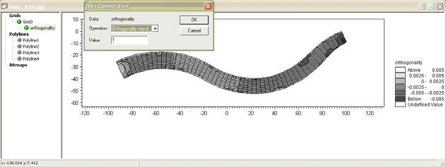
1.8.3 Data . . . . . . . . . . . . . . . . . . . . . . . . . . . . . . . . . . 45
1.8.4 Polylines . . . . . . . . . . . . . . . . . . . . . . . . . . . . . . . . 46
1.8.5 Bitmaps . . . . . . . . . . . . . . . . . . . . . . . . . . . . . . . . . 47
1.8.6 Mouse operations . . . . . . . . . . . . . . . . . . . . . . . . . . . 48
2 Example . . . . . . . . . . . . . . . . . . . . . . . . . . . . . . . . . . . . . . . . 51
2.1 Introduction . . . . . . . . . . . . . . . . . . . . . . . . . . . . . . . . . . . 51
2.2 Ideas and Theories behind MIKE 21C Grid Generator . . . . . . . . . . . . . 51
2.2.1 General guidelines . . . . . . . . . . . . . . . . . . . . . . . . . . . 51
2.2.2 Polylines . . . . . . . . . . . . . . . . . . . . . . . . . . . . . . . . 52
2.2.3 Grids . . . . . . . . . . . . . . . . . . . . . . . . . . . . . . . . . . 53
2.2.4 Grid update . . . . . . . . . . . . . . . . . . . . . . . . . . . . . . . 55
2.2.5 Derived grid information . . . . . . . . . . . . . . . . . . . . . . . . 59
2.3 Before Starting this Tutorial... . . . . . . . . . . . . . . . . . . . . . . . . . . 61
2.3.1 Files to start with . . . . . . . . . . . . . . . . . . . . . . . . . . . . 62
2.3.2 Additional file . . . . . . . . . . . . . . . . . . . . . . . . . . . . . . 62
2.4 Create Tutorial Curvilinear Grid . . . . . . . . . . . . . . . . . . . . . . . . . 62
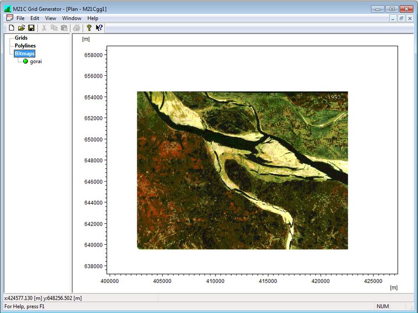
2.4.1 Import background image and river outline . . . . . . . . . . . . . . 62
2.4.2 Grid generation strategy . . . . . . . . . . . . . . . . . . . . . . . . 64
2.4.3 Bifurcation . . . . . . . . . . . . . . . . . . . . . . . . . . . . . . . 65
2.4.4 Grid resolution . . . . . . . . . . . . . . . . . . . . . . . . . . . . . 65
2.4.5 Grid generation methodology . . . . . . . . . . . . . . . . . . . . . 66
2.5 Generate Bathymetry . . . . . . . . . . . . . . . . . . . . . . . . . . . . . . 73
Index . . . . . . . . . . . . . . . . . . . . . . . . . . . . . . . . . . . . . . . . . . . . . .79
6 MIKE 21C Grid Generator - © DHI A/S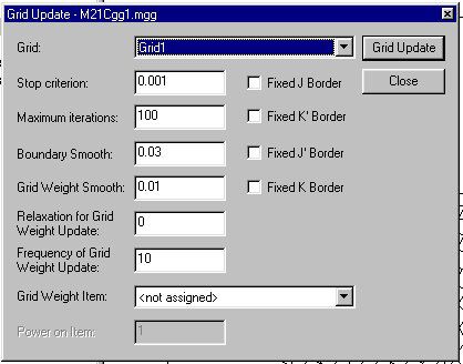
Introduction
1 Reference Manual
The grid generator contains three main properties: Grids, Polylines and Bit-
maps. A typical project encompass the following activities:
Import a Bitmap file as background image for orientation
Generate Polyline describing bank lines based on background image
Generate grids based on polylines
Add data items to the generated grid
There are four basic functions for grid generation:
New Grid
Merge Grids
Add Grid
Options for grid
The functions are activated by selecting Grids with the mouse and right-click.
Addition functions (Grid Operations) are available for each grid in the project.
These functions are activated by selecting the relevant grid with the mouse
and Right-click.
1.1 Introduction
The MIKE 21C Grid generator is used to create and modify data defined in
curvilinear grids with the following file formats: *.dfs2, and *.dt2 (ie - 2D binary
data files in association with DHI Software). These files typically contain the
model bathymetry, bed resistance data, etc. A brief introduction to grid gener-
ation is provided in this section:
The difference between a rectilinear and a curvilinear grid is depicted in
Figure 1.1.
Powering Water Decisions 7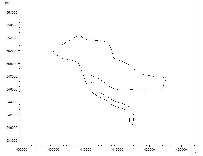
Reference Manual
Figure 1.1 Left: A rectilinear (standard) MIKE 21 model. Right: A curvilinear MIKE
21C model
In contrast to a rectilinear MIKE 21C 2-D data file, an additional 2-D file with
the position of the grid points (in the following referred to as the grid file) must
supplement the curvilinear MIKE 21C 2-D data file. Both files are based on
the dfs2 or the dt2 format meaning that the usual MIKE 21 tools such as the
Grid Editor can be applied to the curvilinear files as well.
Input for the MIKE 21C Grid generator is background images showing the
study area, text files with position of e.g. bank lines (x,y data) and text files
with bed elevation at discrete points (x,y,z data). Output from the MIKE 21C
Grid generator is
A grid file *.dfs2 with the position of all grid points (x,y)
A bathymetry file or data file *.dfs2 with the value in each grid point (z)
A curvilinear grid is generated to cover the entire model area, i.e. the area
where information about bathymetry is available and model results are
required. The MIKE 21C model bathymetry is in a matrix format with each
value representing the mean bed level within a grid cell, see Figure 1.2. The
four corner points define the grid cells. The dimensions of the grid matrix will,
therefore, be one higher in each direction than the corresponding bathymetry
matrix. If for instance the bathymetry matrix has the dimension 100x100 the
corresponding curvilinear grid will have 101x101 grid lines.
8 MIKE 21C Grid Generator - © DHI A/S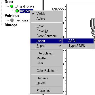
Introduction

                     Figure 1.2    Definition sketch of curvilinear grid

                     Note, that the grid file is a special type of dfs2. Grid point information is saved
                     by double precision in two static items, and by single precision in two dynamic
                     items. Only the dynamic items can be viewed in the ‘Tabular View’. If values
                     are modified in the MIKE Zero Grid Editor (by default the Grid Editor starts
                     when a dfs2/dt2 file is loaded into the MIKE Zero interface), the double preci-
                     sion information will be lost. The MIKE 21C engine will apply the double pre-
                     cision information is it is available (i.e. two static items written in the grid file),
                     otherwise the single precision grid coordinate will be applied. For grids with
                     relatively small cells and e.g. UTM coordinates (or similar large x- and y-val-
                     ues) application of double precision is essential for calculating the spacing
                     functions ds and dn with sufficient accuracy. As a rule of thumb the inaccu-
                     racy in the spacing functions is around 10-6 compared to the grid coordinates
                     if using single precision, while the inaccuracy is practically non-existent for
                     double precision coordinates.

                     The Grid Generator always stores the coordinates in double precision, i.e. if
                     using the Grid Generator one never has to worry about the precision of the
                     grid coordinates.

1.1.1     Start of new application

                     m21gg.exe activates the MIKE 21C Grid Generator.

                     When the MIKE 21C Grid Generator is started without an existing grid, the
                     user is prompted for the coordinates defining the extent of the study area:

Powering Water Decisions                                                                                  9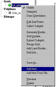
Reference Manual
If at a later stage an existing grid file is imported with a bigger extent, the
graphical view will automatically be updated. The same applies if a bitmap is
imported. Using the View and Settings it is possible at a later stage to update
the plan view.
The grid generator contains three main properties: Grids, Polylines and Bit-
maps. A typical project encompass the following activities:
Import a bitmap file as background image for orientation
Generate polylines describing bank lines based on background image
Generate grids based on polylines
Add data items to the generated grid
The various functions for the three main properties (grids, polylines and bit-
maps) are activated by right-click of the mouse, see example below.The func-
tions with the mouse button are description under options.
10 MIKE 21C Grid Generator - © DHI A/SIntroduction
1.1.2 Creating a new grid
The creation of a curvilinear grid is divided into four parts:
Bitmap import used for background image
Polyline creation based on data or digitisation of bitmap
Grid creation based on defined polylines
Data map creation based on defined grid
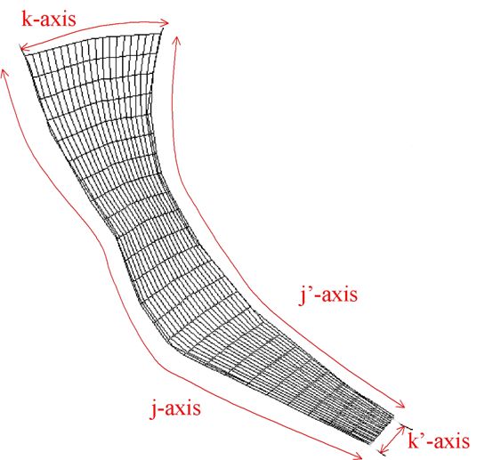
The curvilinear grid is defined by 4 borderlines. There are called the J, J’, K
and K’ line as shown below. The MIKE 21C grid has to be orthogonal mean-
ing that also the borderlines must meet at right angles. A curvilinear grid is
defined using the "New Grid" function.
Figure 1.3 Definition of border lines
Border lines are defined as polylines. Polylines can be digitised directly on
top of a background image by using the "New Polyline" function, or they can
Powering Water Decisions 11Reference Manual
be imported from data files (using the "Add Polyline from File" or "Import
Polyline from DAT/XYZ file".
Background images are displayed graphically by using the "Add Bitmap from
File" function.
The numbering of grid points follow the definition of the borderlines, as the
point (j,k)=(0,0) is at the lower left corner where J and K line meet, and the
point (j,k)=(jmax,kmax) is at the upper right corner where the J’ and K’ line
meet.
The distribution of the (j,k) points in the interior of the grid is determined by
the solution of a set of elliptical equations expressing the orthogonality of the
grid, see Grid Orthogonality. After creation of a new grid, the grid points are
"orthogonalised" using a "Grid Update"-function.
Often, it is desirable to shape the grid in a particular way around islands in the
middle of a river, bifurcations and channel confluences. This is possible by
dividing the grid into smaller grid parts from the beginning. Each grid part is
defined and orthogonalised independently and subsequently merged
together into one large grid.
Figure 1.4 Planning of grid parts to be orthogonalised before merging
1.1.3 Modifying a grid
Corrections and modifications to an existing grid can be done. When a grid is
divided into multiple parts, it is important to be able to split the work into parts
and be able to take backups of each part. Various import facilities exist for
this:
Data maps can be imported from/exported to *.dfs2 files
Grid files (entire or parts of the grid) can be imported from /exported to
*.dfs2 files
12 MIKE 21C Grid Generator - © DHI A/SIntroduction
Sub-grid files can be extracted and/or merged
Polylines defining border can be imported from /exported to data files
Sub-polylines can be extracted and/or merged
The Grid Editor for MIKE 21 is applied for standard *.dfs2 files, but can also
be applied to change either the data files or the grid files.
Data or grid files defined in other curvilinear format than MIKE 21C can be
converted into ASCII text file format, imported to a *.dfs2 file using the Grid
Editor in MIKE 21 and subsequently be imported to the MIKE 21C Grid gen-
erator. Similarly, the files generated by MIKE 21C grid generator can be
exported as ASCII files using the Grid Editor in MIKE 21.
1.1.4 Grid orthogonality
The theoretical background for the grid generator is outlined below. Refer to
"Gridgen - Scientific background" for further details. The orthogonal curvilin-
ear grid is obtained by solving the following elliptic partial differential equa-
tions:
-----x --1- -----
x-
g + = 0
g
(1.1)
-----y --1- -----
y-
g + = 0
g
where
x,y Cartesian coordinates
, curvilinear coordinates (anti-clockwise system)
g “weight” function
The weight function is a measure of the ratio between the grid cell length in
the x - and the y -direction, respectively. It is defined through the following
relationships:
g 11
g = ------
- (1.2)
g 22
Powering Water Decisions 13Reference Manual
where
2 2
x y
g 11 = ----- + -----
(1.3)
2 2
x y
g 22 = ------ + ------
The elliptic grid equations are solved using an implicit finite difference approx-
imation and Stone's strongly implicit procedure (abbr. SSIP, see Stone, 1968).
The input for the grid generator is the grid weights, g, in every grid point and
the boundary conditions in terms of a set of (x,y) co-ordinates for each of the
four boundary lines. The output from the grid generator is the (x,y) co-ordi-
nates of the grid line intersection points. With the present MIKE 21C grid gen-
erator, the grid weight g is not defined explicitly as input. Instead g is
calculated from the initial grid point distribution, and subsequently filtered
based on user-defined parameters.
Generation of an orthogonal curvilinear grid is an iterative process in which
boundaries are smoothened and weight functions are adjusted until the com-
putational grid is judged to be sound, i.e. be orthogonal with sufficiently grad-
ual transitions. Use of graphical facilities is an important tool in assessing the
quality of the generated grids.
1.1.5 Specifications for grid generator
The specifications applied for each MIKE 21C Grid generation can be stored
for later use.
To save M21 Grid Generator setup with all the parameters for the grid gener-
ation, go to File Save or Save As and select file name for the parameter file
you want to save.
To open an existing setup file, go to File - Open and select the file format that
you are looking for.
When you have selected the setup to edit, the editor is ready to work. Similar
to other MIKE Zero editors, a parameter file is associated with the application.
In this case, the extension of the parameter file (text file format) is *.mgg.
1.2 New Grid
Specification of a new grid requires that 4 borderlines are available. In the
example below, the existing borderlines are Polyline1, Polyline2, Polyline3,
and Polyline4. The borderlines are displayed in the graphical view.
14 MIKE 21C Grid Generator - © DHI A/SNew Grid
1.2.1 Specifications
Result Grid
If is specified the grid generator will generate a new file. Oth-
erwise, browse to the name of an existing grid file that will be overwritten.
Border 1 (J)
Browse to the selected polyline. This border is between (j,k) = (0,0) and
(jmax,0).
Border 2 (K’)
Browse to the selected polyline. This border is between (j,k) = (jmax,0) and
(jmax,kmax).
Border 3 (J’)
Browse to the selected polyline. This border is between (j,k) = (0,kmax) and
(jmax,kmax).
Border 4 (K)
Browse to the selected polyline. This border is between (j,k) = (0,0) and
(0,kmax).
Interpolation
There is one option: Bilinear interpolation. The interpolation defines the type
of the initial grid, which will be generated using the "Generate" function. This
initial grid is non-orthogonal (orthogonalisation is performed later in "Grid
Update").
Points JxK
Press the "…" button to define the grid size.
Powering Water Decisions 15Reference Manual
1.2.2 Action buttons
Generate
The initial grid is generated as specified. If the result grid name is a control box appears to confirm that a new grid has been gener-
ated and added to the project:
Snap
Adjacent polylines should match at the corner points. However, due to accu-
racy, it will never be completely fulfilled. With the "snap" functionality a new
common end point is defined between the two end points which were sup-
posed to be identical.
Edit Points
After the size of the grid has been defined, the grid generator will automati-
cally distribute points uniformly along the four borders. Interpolation will take
place between these points for the initial grid. Using the Edit Point functional-
ity, it is possible to make a non-uniform point distribution along the borders. At
each border line, use the "…" button to enter "Edit Point" properties. Define
control points, which are distributed depending on the existing distribution of
points. Use "Edit Points" to move all points between the control points along
the border graphically.
16 MIKE 21C Grid Generator - © DHI A/SMerge Grids
1.3 Merge Grids
In simple cases it is sufficient to generate one grid. However, if a study area is
more complicated (perhaps with an island in a river channel), it is necessary
to split the grid into grid parts and prepare each part separately. The figure
below shows an example of a grid generation project, which has been divided
into 9 different parts.
The purpose of this function is to merge two grids with identical numbers of
points along the common border. Before the two grids are merged, they must
be prepared separately using New Grid and (but not necessarily also) Grid
Update. As discussed below, it is important that the points along the common
Powering Water Decisions 17Reference Manual
border between the grids to be joined are coincident. Therefore, the same
polyline is usually applied for generating each grid. In addition, the common
border is usually fixed when Grid Update is applied for each of the grid parts.
This will ensure that the points along the border coincide in both grids.
Figure 1.5 User dialog for merging the grids
Grid 1 and Grid 2 contain the names of the two files to be merged. The input
for the Result Grid can be either or the name of an existing
grid file in the project. In the latter case, that grid file will be overwritten with
the new merged grid.
In principle, the points along the common border should be exactly the same.
In practice, the points can be different because of each of the two grids has
been orthogonalised, which will cause the grid points along the border to
move. The allowed max difference between two points, which were supposed
to be identical, can be specified here. If the points are still too far apart, an
error message will occur:
If the thorough border test is activated, the points must be exactly the same
along the common border.
1.4 Add Grid
An existing grid file (*.dfs2 or *.dt2 format) can be imported into the grid gen-
erator. The purpose can be to
Modify the grid
18 MIKE 21C Grid Generator - © DHI A/SGrid Operations
Merge the grid with another
Add items to the grid (e.g. bathymetry)
Figure 1.6 Add grid from file dialog
1.5 Grid Operations
The following operations (right-click selected grid in the project) can be per-
formed on the grid:
Powering Water Decisions 19Reference Manual
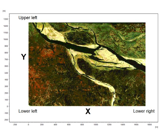
1.5.1 Draw grid orientation
The curvilinear grid prepared for MIKE 21C is oriented according to the direc-
tion of the J-lines and K-lines. Usually, the following orientation is applied: J=0
at the upstream boundary and J=max at the downstream boundary.
The orientation is shown with letters and colour codes as depicted below. In
this case (J,K)=(0,0) at (x,y)=(-60,-14) at the upstream boundary. In the
downstream boundary, (J,K)=(19,0) at (x,y)=(10,-60) approximately.
20 MIKE 21C Grid Generator - © DHI A/SGrid Operations
1.5.2 Edit grid points
After completion of grid generation, the user has a possibility to move few
points manually by using this function. With the mouse, it is possible then to
select and drag the grid points graphically in the view section.
The function is useful if grid points have to match exactly to certain points in
the interior of the modelling area.
1.5.3 Select subgrid
Selection of subgrids is important for various reasons
In connection with orthogonalisation of subareas: Grid Update will only
operate on the selected subgrid.
In connection with modification of data item: Operations on data will only
be effective within selected subgrid.
In connection with extraction of a subgrid: The selected subgrid will be
extracted.
Powering Water Decisions 21Reference Manual
After pushing the Select Subgrid button, see below, the user can mark the rel-
evant area graphically with the mouse. In order to see the actual selection, it
may be necessary to update the options for display of subgrid.
1.5.4 Generate border
With this function, a polyline can be extracted from an existing grid file.
22 MIKE 21C Grid Generator - © DHI A/SGrid Operations
Grid specifies the name of the grid in the project, from which a border line
(polyline) should be extracted or generated.
Grid Border specifies from which side of the existing grid, the border should
be extracted. It can be one of the four sides but not from the interior of the
grid. Thus Grid Border can be J, J', K or K' (see definition of alignment in the
introduction).
If Extract border part is selected, the start point and the end point must be
specified, either directly in the table (From and To) or graphically by using the
mouse in the view window after pressing the "…" button.
The Save to Border works together with the New Grid-dialog, see below.
If Save to Border is specified as J, then it correspond to Border 1 (J) in the
dialog above and the name of the extracted border liner will be "Polyline1"
because that is the name displayed in the New Grid-dialog. Thus, the function
should be used with caution, as any existing polyline stored under the name
will simply be replaced by the new data from the Generate Border application.
Powering Water Decisions 23Reference Manual
If in this case the Border 1 (J) input in New Grid-dialog is , the
grid generator will automatically assign a new name to the extracted border
line (polyline) and place the name in the Border 1 (J) input.
1.5.5 Grid update - orthogonalisation
The MIKE 21C flow model engine requires that the curvilinear grid is orthogo-
nal. The present function will activate a grid generator engine, which will
orthogonalise the grid by solving a set of elliptical equations (see Grid orthog-
onality (p. 13)). The grid update (orthogonalisation) operation is often applied
in connection with Select subgrid. Only grid points within the selected subgrid
will be modified.
Stop Criterion and Maximum Iterations
The solution is found by iteration, where the user must specify the stop crite-
ria for convergence Stop Criterion. The default value is 0.1% (=0.001)
change from one iteration to another in average for all grid points. The user
also defines an upper limit of the number of iterations (default is Maximum
Iterations = 100).
24 MIKE 21C Grid Generator - © DHI A/SGrid Operations
Boundary Smooth filter
In principle, the grid points along the borders must be movable in order to
obtain convergence of the solution of the elliptical equations. The grid gener-
ator calculates the position of the points along the border by extrapolating
interior points perpendicular to the border. If the border is curving too much
compared to the density of interior grid points, there is a risk that the grid will
not converge. Therefore, a filter Boundary Smooth is applied to the curva-
ture of the border line. If the curvature of the border line (=1/Radius) is more
than the specified value, the border points will be smoothed. Thus, the
smaller value, the more smoothening of the border lines.
Grid Weight Smooth filter
The grid weights q expressing the ratio of the width and length of each grid
cell will be the same throughout the iteration towards a solution. The grid
weight is calculated at the very first iteration based on the initial grid. The grid
weight can vary throughout the grid domain. A high variation in grid weights
represents a quite non-uniform grid, whereas a small variation indicates a
smooth grid. For numerical reason in the MIKE 21C flow model engine, a
smooth grid is preferred. Therefore, the user can specify a critical value for
the variation in the grid weights. If the grid weight at a point minus the aver-
age of the neighbouring points is more than the specified Grid Weight
Smooth value, the grid weights will be smoothed. Thus, the smaller value,
the more smoothening of the grid.
Recalculation of Grid Weights
As mentioned, the elliptical model require that the grid points along the bor-
ders must be movable in order to obtain convergence of the solution of the
elliptical equations (see Grid orthogonality (p. 13)). However, in some circum-
Powering Water Decisions 25Reference Manual
stances, it is necessary to fix one or more of the borders. This is the case if
the user want to orthogonalise a subgrid only. Thus, if points along the bor-
ders are fixed, the remaining degree of freedom is the grid weight in the inte-
rior of the model. This function allows the user to recalculate the grid weights
during the iteration.
The parameter Relaxation for Grid Weight Update represents the relaxa-
tion parameter:
If value = 0 the grid weights are fixed throughout the simulation.
If value = 1 the grid weights are updated based on recalculated values.
If value = 0.8 (for instance) the grid weights are updated based on a
weighted value of the old grid weight and the recalculated value.
The parameter Frequency of Grid Weight Update specifies the frequency
by which the q-values are updated:
A value =1 will update the grid weights at every iteration time step, but
will also slow down the iteration considerably.
A value = 10 will update the grid weights at every 10 iteration time step,
and is usually sufficient.
The filter on the grid weights (Grid Weight Smooth) is also active when the
grid weights are recalculated. However, if the filter is too fine (smooth grid) it
can be difficult to obtain an orthogonal grid as the filter together with the fixed
borders puts a constraint on the degree of freedom for the grid to adjust.
Thus, there is a compromise between how smooth the grid is, and how
orthogonal the grid is.
Grid weight item
By default, the initial grid weights q expressing the ratio of the width and
length of each grid cell are calculated from the initial grid. There is an option,
however, to let the grid weight be a function of the value of a data item. This is
useful if for instance the grid weight should be a function of the local depth,
velocity field, concentration field or similar. The only requirement is that the
particular Add item is associated with the grid. In such case, the grid genera-
tion will be an iterative process as the item can not be associated with the
grid before it is completed, and the grid cannot be complete until the data
item has been defined.
Fixed borders
If a sub-grid is orthogonalised, it is important to specify that the border points
are fixed along the borders towards the surrounding grid. Otherwise, the grid
orthogonality in the adjacent points in the surrounding grid will be destroyed.
As a rule of thumb, Relaxation for Grid Weight Update should be larger
than 0 to obtain orthogonality when the borders are fixed. In this case, the
26 MIKE 21C Grid Generator - © DHI A/SGrid Operations
Grid Weight Smooth should be adjusted by trial and error until an accept-
able trade off balance between 1) fixed borders, 2) distortion of grid cell sizes
and 3) orthogonality is achieved.
1.5.6 Extract subgrid
An existing grid can be split up into subgrids in the following way:
1) Right-click on the grid and select a subgrid
2) Right-click on the grid and choose Extract Subgrid
Source Grid is the name of the grid from where the subgrid is extracted.
Size J x K is information about the source grid.
Result Grid contains the name of the extracted subgrid. If is
applied, the MIKE 21C Grid generator will invent a name.
Powering Water Decisions 27Reference Manual
Extract executes the operation.
1.5.7 Resize grid
The Resize Grid function creates a new grid with user-specified number of
grid points. The grid generator will interpolate in the existing grid in order to
find the position of the new grid points in the interior of the grid.
The function is useful in connection with development of grids with a higher
resolution without having to redo the entire grid generation. The grid orthogo-
nality will be maintained (down to certain accuracy).
28 MIKE 21C Grid Generator - © DHI A/SGrid Operations
1.5.8 Add land border
The grid generation is usually based on polylines which follow the bank lines.
The computational engine, however, requires one extra row of land cells
defining the banks and the border between water and land. The "Add Land
Border" facility can be used to add an extra grid line to the generated grid
covering the water area only. The application will simply extrapolate the grid
points along the bank line to the new row of grid points on the bank.
The result of this operation is a new grid with the added grid lines along the
specified borders J, J', K and/or K'.
Later during "Add item", the bathymetry values in these new additional grid
points along the channel should be defined above the defined land value (see
Properties (p. 35)).
1.5.9 Grid info
The function displays the information about the current grid:
Size (number of points in the J and the K direction)
(x,y) coordinate at the origin (j,k)=(0,0), lower upstream
(x,y) coordinate at the lower downstream (j,k)=(jmax,0)
(x,y) coordinate at the upper upstream (j,k)=(0,kmax)
(x,y) coordinate at the upper downstream (j,k)=(jmax,kmax)
Powering Water Decisions 29Reference Manual
1.5.10 Add item
The grid files contain information about the horizontal coordinates (x,y). Use
this function to associate an item with the grid, such as bed elevation (z) or
bed resistance (M, n, C).
The data item is stored in a separate file. Thus, complete information about
(for instance) bed bathymetry is contained in two *.dfs2 files (or *.dt2 files).
Relevant operations on the data items are described in Items (p. 31).
30 MIKE 21C Grid Generator - © DHI A/SGrid Operations
In most applications a GIS is used at the principal data storage and mainte-
nance tool. For generation of a bathymetry item, the following options exist
Export the grid cell-centre locations to a GIS containing a DEM, interpo-
late depths onto the points, then re-import the updated points into the
MIKE 21C Grid Generator;
Import a file of XYZ data from a GIS (or other source such as MIKE Zero
Bathymetry Editor) into the MIKE 21C Grid Generator and interpolate the
depths onto the grid points; or
Manually insert the bathymetry using the DT2 editor tools in MIKE Zero
using Cartesian coordinates (not curvilinear).
1.5.11 Add item from file
A new item can be imported from an existing curvilinear data file (dfs2) of the
same size, i.e. corresponding to the grid, to which the item is added.
1.5.12 Items
Active item
Colour contours of the data item and a colour legend can be displayed in the
View Window. However, as only one item can be displayed at the time, the
user can define whether the item is active or not. This is important when more
than one item has been defined.
Save - save as
The generated data item can be stored in a separate *.dfs2 file or *.dt2 file by
using this function. The user specifies the name of the new file.
The size of a data item file (z) is always one less than the size of the grid file
(x,y). The reason is that the z-value is cell-centred whereas the xy-values are
node centred. This is illustrated below, where each computational cell in
MIKE 21C is surrounded by four xy coordinates describing the corner points.
Powering Water Decisions 31Reference Manual
Clear
The data item within the grid will be reset (to delete value). The operation is
often applied in connection with Select subgrid. Only values within the
selected subgrid will be deleted.
Import
The data item can be imported in different formats
ASCII file, the data will be imported from three columns with (x,y,z) and
placed in the curvilinear grid. Notice that there are no units associated
with the xyz data from an ASCII-file, so you have to specify the units for
xy and z data, respectively, before loading the ASCII file. If more than
one discrete value appears within one grid cell, the average of these val-
ues will be computed before import to the grid cell.
Rectilinear Dfs2 file, the data will be stored in a standard rectilinear file
(not yet implemented)
Curvilinear Dfs2 file, use the Add item from file command
Export
The data item can be exported in different formats
ASCII file, the data will be stored in three columns with (x,y,z). If a sub-
grid is selected, only the values within this grid is stored in the ASCII file
Rectilinear Dfs2 file, the data will be stored in a standard rectilinear file
(not yet implemented)
Curvilinear Dfs2 file, use the Save - save as command
Interpolate
Missing data can be interpolated using three different kinds of interpolation
routines.
32 MIKE 21C Grid Generator - © DHI A/SGrid Operations
J interpolation - searching for points along the J-lines only (longitudinal
direction)
K interpolation - searching for points along the K-lines only (transverse
direction)
Elliptical interpolation - Searching within an ellipsoid
Often, bed levels in e.g. a river are available in cross-sections with a certain
distance. In such a case, K interpolation can be used to close gaps in each
cross-section. This operation is followed by J interpolation, which will close
the gap between the cross-sections.
More interpolation operations are possible if the data item file is loaded into
the Grid Editor in MIKE Zero.
Modify
Different operations are available for modifying the data. The operations are
usually applied in connection with Select subgrid. Only values within the
selected subgrid will be modified.
Powering Water Decisions 33Reference Manual
Available operations:
Orthogonality check
Spacing ds
Spacing dn
Area A
Set Value
Add Value
Multiply Value
More operations are possible if the data item file is loaded into the Grid Editor
in MIKE Zero.
Filter
Data can be smoothed. The operation is often applied in connection with
Selection of Subgrids. Only values within the selected subgrid will be
smoothed using the relationship: Zj,k = (Zj+1,k + Zj-1,k + Zj,k + Zj,k+1 + Zj,k-1)/5
More smoothing operations are possible if the data item file is loaded into the
Grid Editor in MIKE Zero.
Colour palette
The colour legend can be changed using the standard MIKE Zero colour pal-
ette Wizard.
A separate colour palette file cannot be saved and loaded in the present ver-
sion of the grid generator. However, the specified colour palette will be saved
together with the *.mgg project file. Thus, when the project is reloaded, the
same settings will appear.
34 MIKE 21C Grid Generator - © DHI A/SPolyline
Rename
The data item will get a default name by the MIKE 21C grid generator (Data1,
Data2, Data3, etc.). Subsequently, the user can rename the data item to e.g.
Bed level, Surface elevations , etc.
Delete
The data item can be removed from the project by using the delete function.
Properties
Most MIKE 21 and MIKE 3 data files have a custom block called "M21_misc".
The bathymetry file in MIKE 21C must contain this custom block. The custom
block can be created and item 4 defined, which is the zland value (see below)
inside the present MIKE 21C Grid generator. Other items in the custom block
can be modified using the Grid Editor in MIKE Zero. The custom block has 7
floating point values:
item 1: orientation at origin relative to true north.
item 2: drying depth.
item 3: code for identifying whether or not the data contains geographical
information; it is -900 if it contains geographical information.
item 4: the zland value, the value above which bathymetric data (the data
itself in case of bathymetry data file; the prefix record containing the
bathymetry in other cases) is considered as land.
item 5-6: are more free and may have different meaning in different situ-
ations.
Right-clicking the Properties of the selected data item generates the follow-
ing dialog, where the user can define the value of land points.
1.6 Polyline
There are nine functions for polyline generation:
New polyline
Powering Water Decisions 35Reference Manual
Merge polyline
Edit polyline
Add polyline from file
Import polyline from DAT/XYZ file
Import polyline from MIKE 11 setup
Show all
Hide all
Options – polylines
The functions are activated by selecting Polylines with the mouse and Right-
click.
Additional functions are associated with each polyline in the project, activated
by selecting the relevant polyline with the mouse and Right-clicking, see
Polyline operations (p. 39):
1.6.1 New polyline
When this menu is selected (right-click on Polylines), a line can be digitised
by left-click on the screen with the mouse. End each line by double-click or by
pressing SHIFT + left-click.
During digitisation, it is still possible to use the right-click for zooming in and
zooming out
36 MIKE 21C Grid Generator - © DHI A/SPolyline
1.6.2 Merge polyline
When this menu is selected (right-click on Polylines), two polylines can be
merged.
Polyline 1 and Polyline 2 contain the names of the two polylines to be
merged. The Result Polyline can have the value , in which
case the grid generator automatically assigns a name. Alternatively, the
name of an existing polyline in the project is provided. Max Difference is the
tolerance for the distance between the two polylines to be merged.
The merging polylines function is particularly useful when long banks are dig-
itised piece by piece.
1.6.3 Edit polyline
This is an option to manually edit the polyline by moving the vertices with the
mouse.
1.6.4 Add polyline from file
Each time a new polyline is created (digitised), the MIKE 21C grid generator
automatically creates a text file with the digitised points. The name of the text
file is + .ggp.
An example of such a text file is depicted below.
Powering Water Decisions 37Reference Manual
The grid generator can import *.ggp files created during an earlier grid gener-
ation process.
1.6.5 Import polyline from DAT/XYZ file
Polylines can be imported from raw text files containing only two columns
with the two horizontal co-ordinates (x,y). An example of such a text file is
depicted below. The extension of the text file must be *.xyz or *.dat
More than one polyline can be imported from the same text file. Each polyline
is separated by a blank line. The user dialog when importing polylines from
*.dat files is shown below. Notice that there is no unit information associated
with a raw .dat/.xyz - file, so you have to specify what metric unit the data
should be interpreted as.
38 MIKE 21C Grid Generator - © DHI A/SPolyline
1.6.6 Import polyline from MIKE 11 setup
This function allows import of bank lines from a MIKE 11 model, which is
done by pointing to the .sim11 file. It should be noted that MIKE 11 models
are usually not as detailed as MIKE 21C models (cross-sections are usually
further apart in MIKE 11 models than the longitudinal grid spacing in an equiv-
alent MIKE 21C model), so the tool should be used with caution, i.e. use for
determining an initial grid for a MIKE 21C model covering the same area as a
MIKE 11 model.
1.6.7 Polyline operations
The following operations (right-click selected polyline in the project) can be
performed on the polyline:
More information is available for the Extract subpolyline functionality.
Powering Water Decisions 39Reference Manual
Extract subpolyline
This function will convert a section of a polyline into a new polyline. This is
useful in situations where (for example) a polyline is available that describes
an entire model domain, and is required for several grids.
In the example above, polyline "Polyline1" consists of 18 digitised points.
The extracted polyline will extend from point 5 to point 8. The "…"-button is
applied to select the points graphically with the mouse. The Result Polyline
can be either (i.e. the MIKE 21C grid generator assigns a
name), or it can be the name of an existing polyline in the project.
The original polyline remains intact.
1.7 Bitmap
Bitmap files are applied to provide background images for grid generation.
This is not a requirement, as polylines may already exist (prepared earlier
using an external application). Bitmap facilities are:
Adding bitmap files to the project
Bitmap operations
Options for displaying bitmap file name
1.7.1 Adding bitmap files to the project
Right-click on Bitmaps:
To Add Bitmap From File, specify the name of the file. Available file formats
include
40 MIKE 21C Grid Generator - © DHI A/SBitmap
*.jpg file
*.tif file
*.bmp file
The placement of the image in the project space needs to be defined. Specify
coordinates of the lower left corner, the lower right corner and the upper left
corner. If a "DHI World File" exists (JPGW or BMPW extension) press Cancel.
After clicking Cancel a Loading coordinate file pop-up box will appear. Here
you have to specify which metrical unit the coordinate from the .jpgw file
should be interpreted in.
Powering Water Decisions 41Reference Manual
1.7.2 Bitmap operations
The following operations (right-click selected bitmap in the project) can be
performed on the bitmap:
42 MIKE 21C Grid Generator - © DHI A/SOptions
1.8 Options
From the MIKE 21C Grid Generator header bar, enter View and Settings.
The display of the
Working Area (Plan),
Grids
Data (grid items)
Polylines
Bitmaps
can be modified with this function. See also Mouse operations (p. 48).
1.8.1 Plan
From the MIKE 21C Grid Generator header bar, enter View and Settings.
The minimum and the maximum X and Y co-ordinates in the working area
can be modified with this function.
Furthermore, the function Globals will search for coordinates of all data in the
project, and return the minimum and maximum X and Y coordinates accord-
ingly.
Powering Water Decisions 43Reference Manual
1.8.2 Grids
The display of grids can be modified with this function. All grids are by default
displayed (normal). The colour and the style of grid lines can be redefined.
For the display of selected subgrids, it is important to be able to distinguish
the subgrid from the main grid. It is possible to define another colour of the
grid lines as well as another line width.
Finally, changing the colour as well as the line width can highlight selected
grids.
44 MIKE 21C Grid Generator - © DHI A/SOptions
1.8.3 Data
The display of the data (grid items) such as bathymetry, bed resistance etc.
can be modified with this function.
Powering Water Decisions 45Reference Manual
1.8.4 Polylines
The display of the polylines can be changed with this menu.
46 MIKE 21C Grid Generator - © DHI A/SOptions
The selection of the option Draw Names is particularly useful during grid gen-
eration, where the appropriate polylines have to be selected.
1.8.5 Bitmaps
The display of the bitmaps can be changed using this menu.
Powering Water Decisions 47Reference Manual
1.8.6 Mouse operations
When the mouse cursor is in the view window, a right-click activates the fol-
lowing functions.
Zoom in, out and use of previous zoom is applied for displaying different lev-
els of details of the grid in the project. Refresh is applied after settings have
been changed. Grid is applied if vertical and horizontal grid lines should be
displayed. The functions Copy to clipboard, Save to metafile, Save to bit-
map are used for storing the display of the grid in another format than on the
screen. The Font changes the font of the numbering of the horizontal and
vertical axes.
48 MIKE 21C Grid Generator - © DHI A/SOptions
When the mouse is in the management window to the left, a right-click will
activate the menus for Grids, Polylines and Bitmaps, respectively.
Powering Water Decisions 49Reference Manual 50 MIKE 21C Grid Generator - © DHI A/S
Introduction
2 Example
2.1 Introduction
This tutorial describes the development of a curvilinear model grid using the
MIKE 21C Grid Generator interface. The grid generated at the end of the
tutorial will be in a format suitable for performing a simulation of MIKE 21C.
The application described is based upon a real problem. The river bathymetry
is shown below:
Figure 2.1 River bathymetry
The model in question consists of a bifurcation in a river. The emphasis of the
study is to assess bank stability issues at the bifurcation. This tutorial will
describe the steps required to develop a curvilinear grid of this river reach
and the bifurcation. More information on the river and bifurcation is provided
in Section 2.4.1.
2.2 Ideas and Theories behind MIKE 21C Grid Generator
2.2.1 General guidelines
Specifics will be described below. However, bear in mind the following points
when creating a curvilinear grid:
The quality of the grid generation affects the quality of the model.
Powering Water Decisions 51Example
The curvilinear grid created at the end of this process is a single grid,
which has a set number of cells in the flow direction (j-coordinate) and a
set number in the transverse direction (k-coordinate). Even if your model
has branches, bifurcations, confluences, or islands it is a single grid that
if straightened out would form a rectangle. However, within that grid
regions of land can be specified.
Model accuracy is reduced when grid cells are not orthogonal and when
the difference in adjacent cell sizes is too great.
Model accuracy is also reduced when grid cells are too coarse or are not
aligned to bed contours sufficiently to accurately describe the bed.
When generating your first grid, save often and expect to make some
repetitions and mistakes.
Grid generation is usually a stepwise process, creating and joining small
sub-grids to make the whole. Try to formulate a strategy before starting,
perhaps on a separate piece of paper.
Remember that the bed levels are not fixed to the grid until grid genera-
tion is complete. At the same time, be aware that a good mesh should be
able to highlight important features of the bathymetry (such as higher
resolution in areas of interest and grid lines following bathymetric con-
tours).
2.2.2 Polylines
A grid or subgrid is defined by 4 polylines that describe the 4 boundaries
(Figure 2.1). The polylines are ordered according to the axes J, J’, K and K’.
A polyline can be created in several ways by right clicking on the Polyline
heading.
52 MIKE 21C Grid Generator - © DHI A/SIdeas and Theories behind MIKE 21C Grid Generator
Figure 2.2 Grid defined by 4 polylines
New Polyline
A new polyline can be traced using the mouse.
Merge Polylines
Two polylines can be merged into a single polyline.
Add Polyline from file
A polyline can be added from another, existing grid generation file. The exten-
sion is “ggp”.
Import Polyline from DAT/XYZ file
A polyline can be imported using the DAT file format. The DAT file is ASCII
(can be read by a text editor) and consists of 2 columns defining the x and y
coordinate. More polylines can be specified for each DAT file by separating
each from another with a blank line in the ASCII file.
More information on polyline operations is available in the Reference Manual,
see 1.6 Polyline (p. 35).
2.2.3 Grids
A grid can be generated in several ways:
Powering Water Decisions 53Example
New Grid
A new grid is created from the four polylines describing the boundaries. Each
polyline is entered in its appropriate border location. Options are available to
Generate a Border, where a polyline defining a border is generated from an
existing grid.
On the bottom of the dialog is the specification of number of points in each
direction. Note that this is the number of points including corners (and not the
number of cells or number of spaces).
Merge Grids
A new grid is created by merging two existing grids together. The tolerance
between grid points at the merging boundary can be specified.
54 MIKE 21C Grid Generator - © DHI A/SIdeas and Theories behind MIKE 21C Grid Generator
Add Grid from File
A grid can be added from another, existing grid generation file containing two
data items: The x and the y coordinate of every grid point. The extension is
dfs2.
2.2.4 Grid update
The Grid Update option orthogonalises and smoothes a grid or a subset of a
grid. This means that the grid is modified so that the angles between succes-
sive grid cells are close to orthogonal (90 ) and grid weights are modified to
be uniform across the grid domain. Grid locations are moved to achieve this.
The option to fix cell locations along each boundary is available.
The Grid Update dialog contains additional options (right). The options are
available to adjust the balance between orthogonalising and smoothing,
which is critical to the successful development of a grid. More information on
each option is provided below
The solution is found by iteration, with a Stop criterion or convergence spec-
ified. Once the average change in grid point positions reaches this value the
Powering Water Decisions 55Example
iterations stop. Otherwise, iterations will continue until the Maximum itera-
tions have been reached.
If the boundary is too curved relative to the interior grid point density, the grid
may not converge. A filter is therefore applied to the curvature of the border
line (Boundary Smooth). If the curvature (1/Radius) is more than the speci-
fied value, the border points will be smoothed. So, a smaller value means a
smoother border. Note this is only applied where a boundary is not fixed.
The grid weight is the ratio between the length and width of a grid cell. For
numerical reasons a smooth grid (or uniform grid weight) is preferred in a
MIKE 21C simulation. Grid smoothing occurs if the grid weight minus the
average of the neighbouring grid weights is more than the specified Grid
Weight Smooth value. So a smaller means a smoother grid.
Grid weight is calculated at the first iteration. Recalculation of grid weights is
done according to the Relaxation for Grid Weight Update and the Fre-
quency of Grid Weight Update. The relaxation factor is similar to an explicit
/ implicit weighting factor:
grid weights are fixed if equal to 0;
grid weights are updated using the recalculated values if equal to 1; and
if equal to 0.8 (for example) grid weights are updated using a weighted
value of the previous and recalculated values.
The frequency factor specifies the frequency that the grid weights are
updated. So a value of 1 means grid weights are updated every iteration, and
a value of 10 means updates every 10 iterations.
To illustrate the grid update, consider the grid:
56 MIKE 21C Grid Generator - © DHI A/SIdeas and Theories behind MIKE 21C Grid Generator
A grid update operation with no borders fixed will give:
A grid update operation with borders fixed will give:
As a rule of thumb, the relaxation for grid weight should be larger than 0 to
obtain orthogonality when the borders are fixed. In such case, the grid weight
smooth should be adjusted accordingly.
Alternatively, set the Stop criterion value to be 0.1, leaving all borders
unfixed. As shown, the grid does not change as much.
Powering Water Decisions 57Example
Try to set the Boundary Smooth value to a small number (say 0.001). The
grid is now unrecognisable:
As can be seen, the final generated grid can be quite different. The option to
Select Subgrid and perform a grid update on the subgrid can be used to per-
form a series of updates at different zones in the grid. In each zone each of
the four boundaries can be selectively fixed or freed. With some iterations the
following grid can be generated:
58 MIKE 21C Grid Generator - © DHI A/SIdeas and Theories behind MIKE 21C Grid Generator
If the grid generation does not produce a suitable mesh using the methods
described above, there are two additional features available:
Edit Grid Points
Points on boundaries and in the interior of the grid can be moved using the
mouse.
Resize grid
The grid can be resized to increase the cell resolution. Note that linear inter-
polation between the existing grid cells is performed.
2.2.5 Derived grid information
When having created a final grid for a specific modelling problem the quality
of the grid should be checked before proceeding to the bathymetry interpola-
tion and the hydrodynamic and morphological modelling. The checks that
should be made are:
Check of orthogonality
Check of spatial spacing gradients in both horizontal directions ds j
and dn k
Check of grid aspect ratio ds/dn
Location of true land cells
Lack of grid orthogonality and too large spatial spacing gradients causes less
accurate results due to violation of the assumptions made for the equations
solved in the flow and sediment transport model. Large spatial spacing gradi-
ents can also be responsible for numerical instabilities in areas with transition
between flooding and drying. The aspect ratio is important in the sense that it
can be used to choose the optimal number of points needed to resolve the
Powering Water Decisions 59Example
flow in the stream wise direction (given the number of points across the
model area). For convection dominated flow problems like river flow aligned
with the curvilinear grid the optimal aspect ratio is in the range from 3 to 8.
For floodplain flow with a less significant flow direction the aspect ratio criteria
should be reduced to the range 1 to 3.
Identification of the true land cells in the bathymetry is important for the
checking of the grid, because in these areas all requirements for grid orthog-
onality and changes in grid size can be ignored, i.e. larger islands in a river
can be resolved with very few grid cells and without being orthogonal, if
defined as a true land area.
In the following the applications for checking of the quality of the grid is
described.
Check of grid orthogonality
The orthogonality check of the grid is made by the following steps:
Add a new item related to the final grid
Right-click on the new added item in the tree on the left and click on
modify
Chose the operation Set value in order to set a dummy value for the grid
Select modify again, but choose now the operation Orthogonality
check
Right click on the added item and click on active. A colour palette will
now be shown to the right and when moving the cursor around on the
grid the x, y coordinates, the value of the item (orthogonality measure),
and the j, k coordinates are shown on the bottom bar.
Save the orthogonality information into a dfs2-file by clicking at Save as
and specify a file name.
For an ideal curvilinear grid the orthogonality measure would be equal to zero
everywhere. However, for practical applications one should try to create a
curvilinear grid with values inside the range from -0.05 to 0.05, depending of
the complexity of the grid. In the example shown below, it is seen that for very
simple grids the criterion given above can be reduced to, say -0.01 to 0.01.
Note, that it is the user that creates the boundary conditions for the grid gen-
erator, i.e. if the polylines have been created so that they not fulfil the orthog-
onality criterion at the corners, it will be impossible to create a satisfactory
orthogonal grid.
60 MIKE 21C Grid Generator - © DHI A/SYou can also read