IIT MADRAS DRDO-STUDENT ROBOTIC COMPETITION - TECHNICAL DOCUMENTATION - ALTERBOT (ALL-TERrain-BOT) 2010
←
→
Page content transcription
If your browser does not render page correctly, please read the page content below
IIT MADRAS
 DRDO-STUDENT ROBOTIC COMPETITION
Military Racing Challenge - Autonomous Ground Vehicle for Low Intensity Conflict

                     ALTERBOT (ALL-TERrain-BOT) 2010

                  TECHNICAL DOCUMENTATION
Contents
1.     Motivation................................................................................................................................................................. 3
2.     Problem Statement (As given by DRDO) ................................................................................................................... 4
3.     Stages of Competition ............................................................................................................................................... 4
4.     Team Members ......................................................................................................................................................... 5
5.     Introduction .............................................................................................................................................................. 6
Bot Development .............................................................................................................................................................. 7
6.1.       iCar ........................................................................................................................................................................ 7
     6.1.1.       Introduction: ................................................................................................................................................. 7
     6.1.2.       Construction and development .................................................................................................................... 7
6.2.       ALTERBOT - Mechanical Module ........................................................................................................................... 8
     6.2.1.       Initial Design .................................................................................................................................................. 8
       6.2.1.1.           Features ................................................................................................................................................ 9
       6.2.1.2.           Specifications ...................................................................................................................................... 10
       6.2.1.3.           Components ........................................................................................................................................ 10
     6.2.2.       Problems faced with the Initial Design ....................................................................................................... 11
     6.2.3.       Final design ................................................................................................................................................. 11
       6.2.3.1.           Side wheel-track belt assembly........................................................................................................... 13
       6.2.3.2.           Main chassis: ....................................................................................................................................... 17
       6.2.3.3.           Design Verification .............................................................................................................................. 18
       6.2.3.4.           Specifications ...................................................................................................................................... 18
       6.2.3.5.           Design Strengths ................................................................................................................................. 18
6.3.       ALTERBOT - Electrical Module............................................................................................................................. 19
     6.3.1.       First Algorithm development ...................................................................................................................... 19
       6.3.1.1.           Macroscopic Level ............................................................................................................................... 20
       6.3.1.2.           Micromanagement Level .................................................................................................................... 20
       6.3.1.2.1.         Tank Mode .......................................................................................................................................... 20
       6.3.1.2.2.         Grass Mode ......................................................................................................................................... 20
       6.3.1.2.3.         Staircase Mode.................................................................................................................................... 20
     6.3.2.       Second Algorithm development ................................................................................................................. 21
       6.3.2.1.           Lane detection .................................................................................................................................... 22
       6.3.2.2.           Obstacle detection (To be finished) .................................................................................................... 28
       6.3.2.3.           GPS based waypoint tracking .............................................................................................................. 32
       6.3.2.4.           Motion planning .................................................................................................................................. 35
       6.3.2.5.           Processing ........................................................................................................................................... 35
       6.3.2.6.           Integration........................................................................................................................................... 36

                                                                                                                                                                        1|Page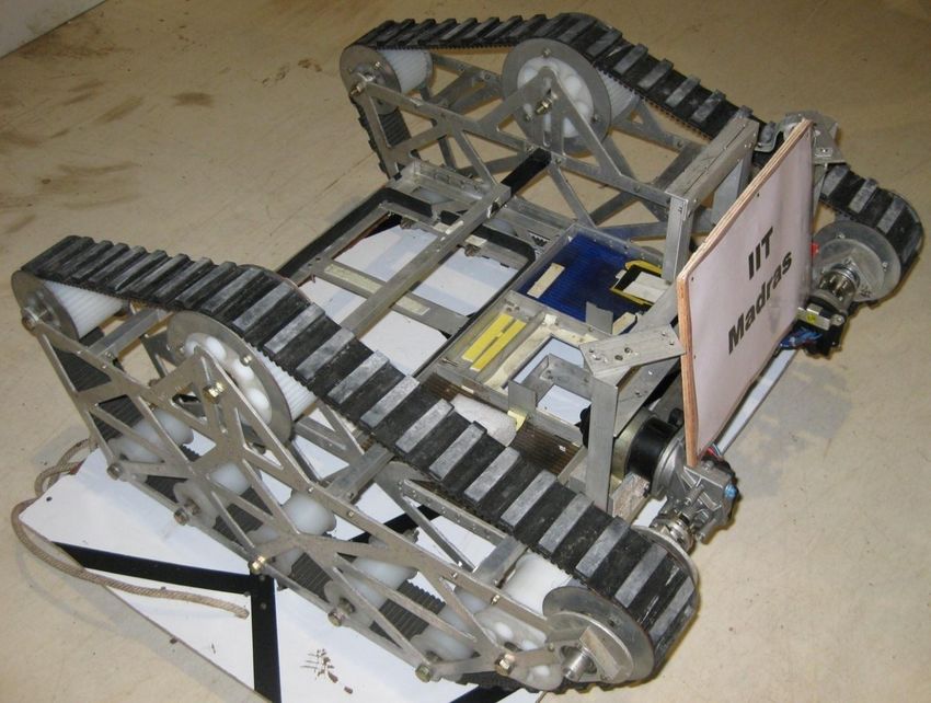
7.    Future Scope ........................................................................................................................................................... 37
8.    Acknowledgements ................................................................................................................................................. 38
9.    References .............................................................................................................................................................. 39
10.      Appendix – I ........................................................................................................................................................ 40

                                                                                                                                                                 2|Page
1. Motivation
In ten years the army will replace troops with ‘Robotic Soldiers’ which will be “autonomous in
all respects.”
--A Sivathanu Pillai, the Chief Controller of India's Defence,
Research and Development Organisation (DRDO)
In today's age when everything is getting automated, one also dreams of an automobile which runs on its own. The
applications of such a vehicle can be widespread.
Help soldiers and public safety professionals.
Help to maintain public safety, keep drivers within the norms, provide wanted emergency medical services
and used for service in inhospitable regions
Carry out unmanned missions like inspection of doubtful objects and other dangerous scenarios from a safe
standoff distance.
It can help minimize risk to military personnel, can be used for surveillance, bomb disposal, and to enter and
secure inaccessible areas by mounting the appropriate module on the robot.
Give complete situational awareness with minimum risk to personnel
Perform dangerous tasks which when done manually would involve great deal of risk to the personnel.
Figure 1: The ALTERBOT
The possibilities are simply boundless
It was this that inspired us to make the ALTERBOT and participate in the DRDO Student Robot Competition – 2010.
The theme for the competition was: “Military Racing Challenge: Autonomous Ground Vehicle for Low Intensity
Conflict."
3|Page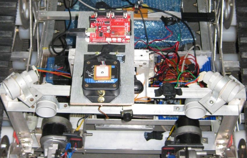
2. Problem Statement (As given by DRDO)
Autonomous ground vehicle has to complete a 500m track which had the following obstacles:
o Gravel of size 2 inches and will be positioned at two different places on the track with a length of 10m each.
o Sand of depth 2 inches and will be positioned at two different places on the track with a length of 10m
each.
o Gradient with an up/down slope of 15 degrees.
o Staircase climbing/descending up to a maximum of 6 steps (rise-7 inches, tread-10 inches).
o 8 corrugations of radius 8 inches and pitch 32 inches.
In the first 350m the robot has to navigate with the help of lane detection, while avoiding all the positive static
obstacles and crossing over gradient and stairs.
The next 150m will be an open area in which the robot has to travel by detecting GPS waypoints which are
provided before start of the competition.
The robot has to carry an additional payload of 10kg throughout the competition.
Facility for wireless E-stop should be provided.
3. Stages of Competition
The competition was held in two stages.
1. A paper on preliminary design.
2. A prototype based on Stage I paper and a detailed design document.
Our team from IITM cleared Stage I of the competition.
The prize money for clearing Stage I was Rs.1, 00,000/- . It was utilized for building the bot.
Stage II of the competition was held at CVRDE, Chennai from 27-29 of September 2010.
Our team from IITM was declared joint winners with other four colleges.
4|Page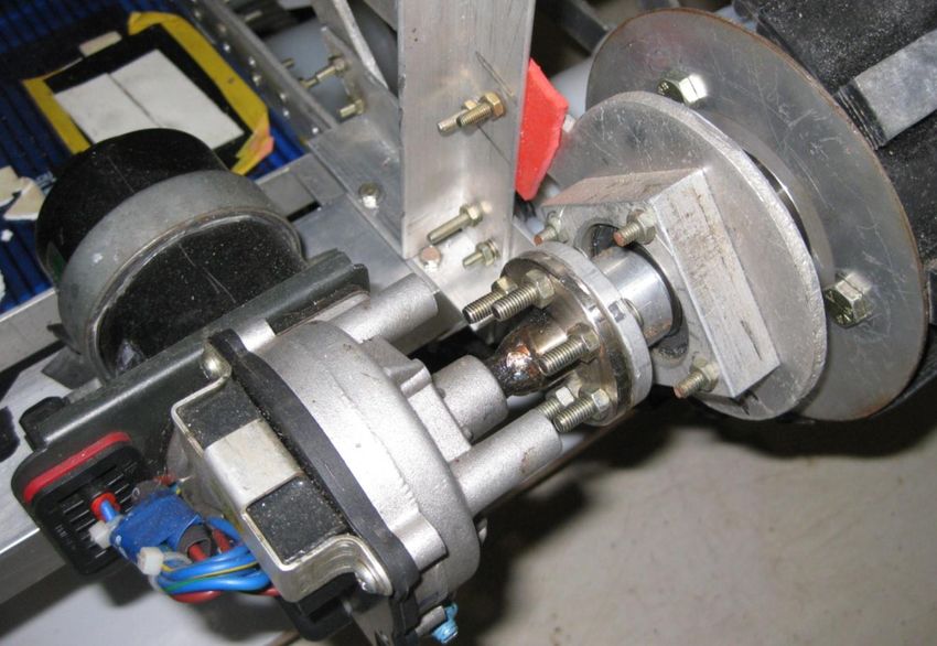
Figure 2: The DRDO SRC - 2010 team
4. Team Members
(From Left)
(Top row)
Nagender VSS – 3rd year, Engineering Design
Anoop Vargheese – 2nd year, Naval Architecture
M Brij Bhushan – 3rd year, Mechanical Engineering
Sanchit Mehta – 2nd year, Metallurgical And Materials Engineering
(Bottom row)
Tanuj B Jhunjhunwala – 2nd year, Mechanical Engineering.
Gaurav Jain – 2nd year, Engineering Design
Vinit S Unni – 3rd year, Engineering Design
Anant Jain – 2nd year, Engineering Design
5|Page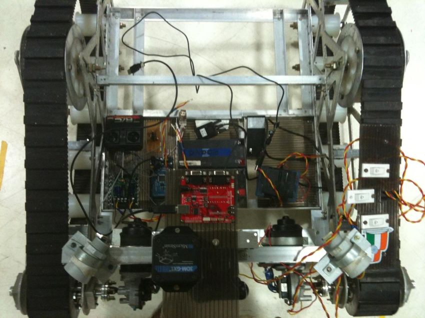
5. Introduction
The ALTERBOT is the product of a 7 month joint effort of a diverse group of IIT Madras Engineering
undergraduate students.
The robot was made under the aegis of the Center for Innovation (CFI) of our institute.
Many design features and innovative solutions to various problems faced were incorporated
In the first round, that involved submission of an abstract; IIT Madras was one the 14 teams that qualified for
the second round out of over 200 teams that participated from all over India in the first round.
The second round involved the fabrication of the robot, and IIT Madras was declared joint winners with
other four colleges.
Figure 3: iCar
6|Page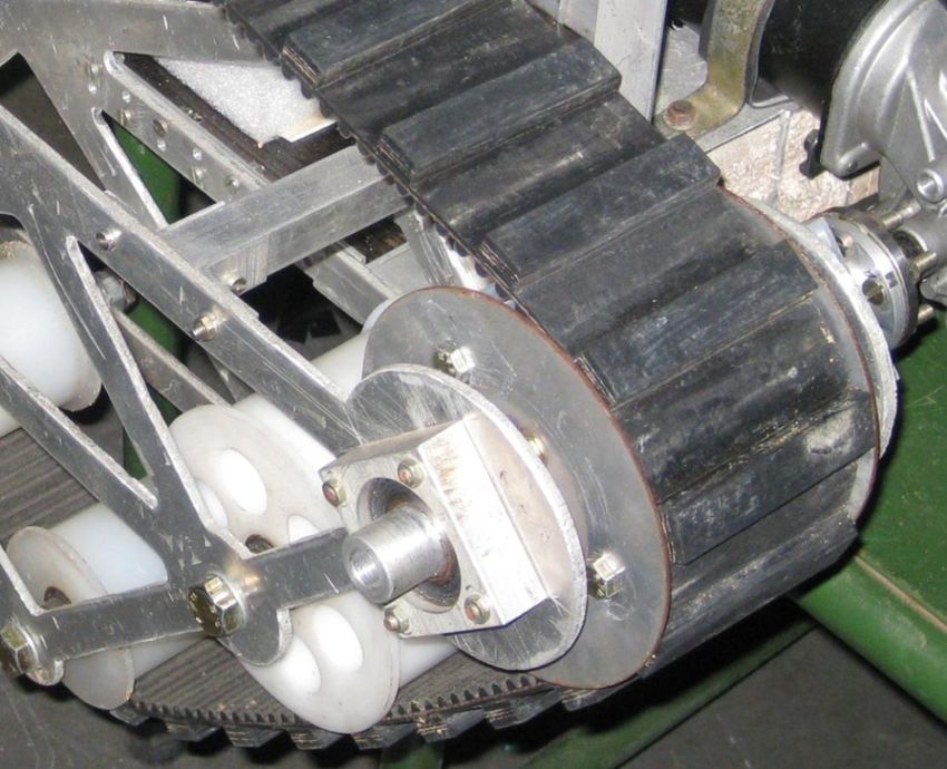
Bot Development

6.1.       iCar

   6.1.1. Introduction:
   The iCar was a student project started at IIT Madras by a team of B-Tech students in June-2009. Their aim
   was to create a robust system that would be able to autonomously travel in real traffic situations, taking
   basic traffic manoeuvres and reaching from point A to point B without any human intervention.

   For this, they incorporated image processing for lane detection and an array of 7 sonar sensors for obstacle
   detection. A camera was used for lane detection. The main processor was an on-board laptop. It was
   inspired by the DARPA Urban Challenge 2007 and their aim was to come up with a low cost scaled down
   version of the same.

   This project provided the team with lots of learning in terms of obstacle avoidance using SONARs, image
   processing and interfacing GPS with a computer.

   6.1.2. Construction and development
   They bought a commercially available toy car (kids’ ride-on car) for our chassis and actuated it. We replaced
   the steering with a servo mechanism and controlled the motor using PWM output.

   They used Maxsonar ultrasonic sensors for the obstacle detection with a range of 6m. They used a single
   camera for lane detection using image processing. The array of sensors mapped a region 150 degrees in the
   front of the vehicle and searched for obstacles and then formed a local map of its environment based on the
   data. This formed the basis of the motion planning after superimposing the data from the lane detection on
   this map.

   For lane detection, we first utilized the image plane transformation, by which we converted the view from
   perspective to an orthogonal view(top view). Then we applied binarization filters for marking out the lanes
   and then by scanning the image from both the left and the right to mark out the lanes. This gives the
   maximum angle that the car is free to move at that instant.

   Each functional module was tested seperately and found to be effective in achieving its objectives.

   iCar was meant to be a completely on-road vehicle and thus its structure was not rugged enough to handle
   off road terrain. Therefore we designed a new platform which will be able to perform in rough and harsh
   conditions.

                                                                                                     7|Page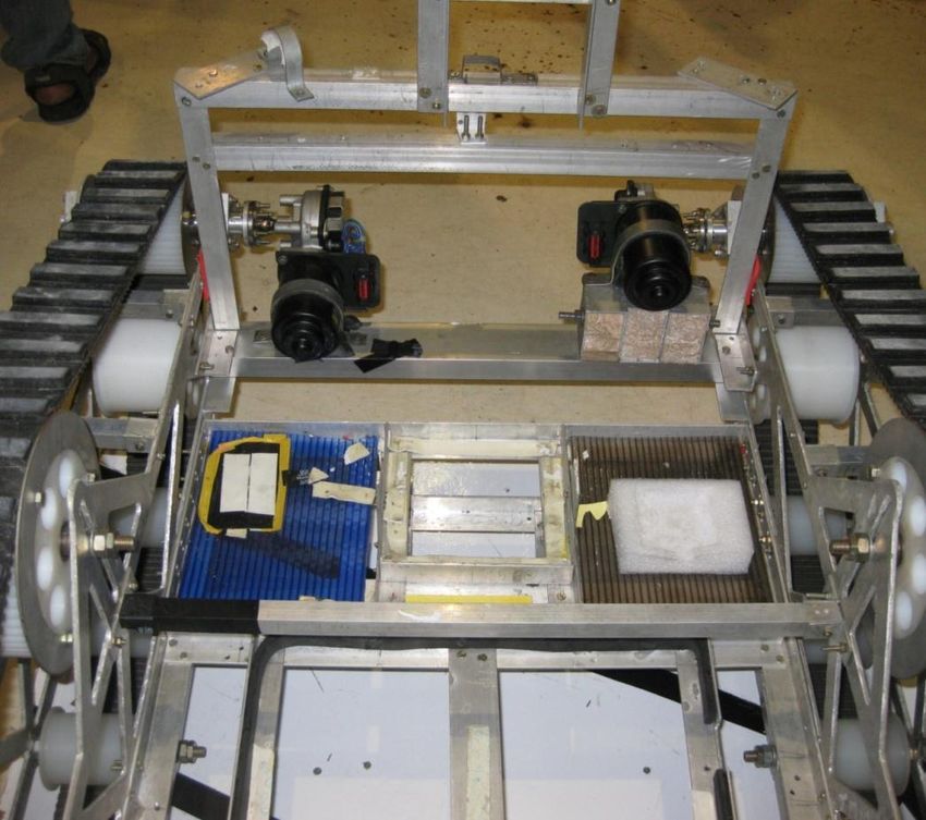
6.2.           ALTERBOT - Mechanical Module
         6.2.1. Initial Design
         The initial design was to make a PACKBOT (used in the US army for surveillance, bomb disposal, and to enter
         and secure inaccessible areas) kind of a robot.

Figure 4: Packbot (iRobot)

Figure 5: First 3D model (Google Sketch-Up)

         The basic structure we used is a tracked vehicle of trapezoidal shape. Outer and inner treaded timer belts
         were the most optimal solution to meet the requirements of climbing stairs and traverse over sand and
         gravel as the weight of the vehicle is more evenly distributed with treads. The problems with using wheels
         was that the weight would only be distributed over a point of contact and thus dig into sand and are also
         susceptible to more wear and tear.

         The flipper was very useful in climbing stairs as the rotatable treads helped in aligning the vehicle according
         to the angle of inclination of the stairs, allowing it to easily climb up. This was achieved by getting the
         flippers into contact with the edge of the bottom stair and applying a torque which aligned the vehicle to an

                                                                                                            8|Page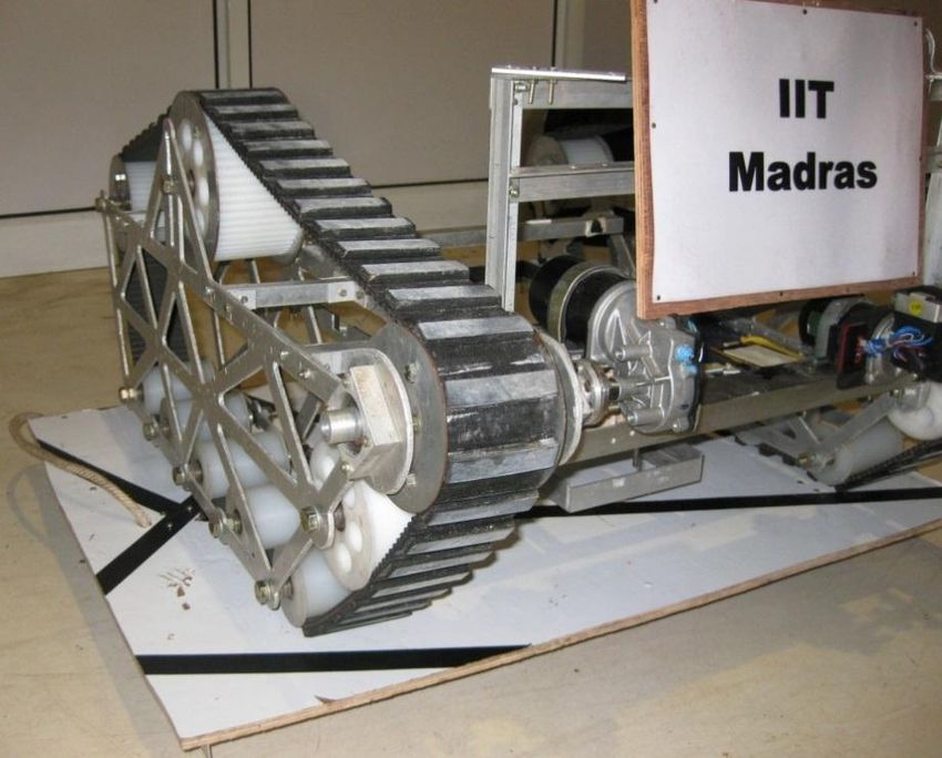
angle at which it climbed on the stairs. While climbing down the stairs, the flipper again played a major role.
The flipper remained in contact with the next stair and when the bot was tilted down the flipper applied a
torque thus reducing the jerk on the vehicle. Angle of the flippers was controlled by a Power window motor
and a potentiometer working simultaneously.
We preferred to use such type of flat treads over larger trapezoidal treads as in this case the center of
gravity of the vehicle will be close to the ground and hence give more stability and maneuverability even
when climbing up slopes or going over stairs or corrugations.
The Robot included:
The main body
The flappers
Figure 6: Prototype - 1
Figure 7: Packbot type design
6.2.1.1. Features
The robot was expected to traverse efficiently over the following terrains:
Sand: The wide 5cm track belt ensured that the robot does not sink into the sand. The robot was
covered on both sides by sandwich aluminium with brushes attached on the edges to prevent sand
from seeping in. The high torque motors drove the polymer belts and helped the robot move over
the terrain. We built a prototype and tested it. The sand was getting stuck between the geared
wheels and the belt, which was the major problem we faced. This was solved by covering the robot
and attaching the brushes.
Gravel: The robot was able to traverse over gravel because we had provided sufficient ground
clearance – greater than 7cm – and high power motors to move the robot efficiently. There were
small support wheels which could freely rotate just above the belt, between the two wheels in the
main body as shown in the design which would prevent the belt from bending and the robot from
getting stuck.
Stairs: The length of the robot was decided based on the dimensions of the steps. The rise of the
steps is 7 inches and the tread is 10 inches. Hence the length of the robot was greater than 27 inches
which was more than twice the length of the hypotenuse which will ensure that there are at least
two points of the robot that are in contact with the surface.
Slope: The polymer belts having teeth on the outer side would provide a high degree of friction,
thus preventing the robot from sliding.
9|PageFigure 8: Prototype 1 – Attachment of power window motor (L) & Full Bot (R)
Figure 9: Prototype 1 - Top view (L) & Idler wheel
6.2.1.2. Specifications
The dimensions of the robot was about 70cm * 60cm, when it is fully extended. It would weigh
around 15 kg. The wheels of the main body had a radius of around 6cm and the smaller wheels at
the front had a radius of about 3cm.
The robot used high torque transmotec motors (24V, 230 rpm, 12 kg-cm) for locomotion which are
provided by the iBot club under Centre for Innovation (CFI). The robot was expected to attain an
approximate speed of 6kmph.
The robot was also expected to carry an additional payload of up to 10 kg.
It was expected to traverse most rugged terrains by altering the alignment of the flappers which
were free to rotate about +/- 120 degrees.
The pitch of the polymer belt was 8mm, as a higher pitch was needed to bear the load of 20kg –
maximum weight of the structure.
6.2.1.3. Components
Based on our ground work on the different materials we could use for our robot, we finally decided to
use Aluminium L- Channels of 3mm for the main chassis. Sandwich Aluminium of thickness 4mm for the
base of the chassis. Wheels were made up of polypropylene. Since it is durable, light and not too
expensive, we had opted for this as compared to aluminium and nylon. The conveyor belt was made up
of a rubber complex. Stainless steel shafts were used for the flanges.
10 | P a g eThe electronics (circuits, batteries, etc.) required would be placed at relevant positions so as to maintain
stability and easy maneuverability of the vehicle.
The electronic components that were expected to be mounted on the vehicle were:
A GPS module
A camera for visual data acquisition.
A LIDAR (Light Detection and Ranging) scanning rangefinder to detect the obstacles.
Digital Compass to find the direction of our heading relative to the GPS waypoint.
Tilt sensors for responding efficiently to slopes, stairs and corrugations.
Encoders to control and limit the speed of the motors
Processing Unit – Gumstix/Laptop
The camera was mounted on a raised swiveling platform so as to provide a good, all-round range of
view. Also, the LIDAR was to be placed in the front portion of the vehicle so that it has an unobstructed
field of view.
The treads were made of high quality rubber which absorbed some of the shocks and also the whole
structure was rigid. Hence, additional suspension system was not required. An additional advantage was
that we were able to take zero radius turns in this sort of a configuration. This would have been a very
difficult task in a wheeled drive and comparatively unstable in a trapezoidal tread system.
The main focus in making the vehicle was to make the system as modular as possible. This helped us in
fabrication as well as testing each component separately.
6.2.2. Problems faced with the Initial Design
We had initially decided on using track belts for locomotion and two front adjustable flappers for extra
support and grip during ascendance. We then made a prototype of this design and tested it and finally had
to disapprove the idea because of various reasons as stated below:
Difficulties in the alignment of track belts.
Severe complications in installing the flappers.
Disappointing performance on sand and stairs.
Sand and other impurities getting stuck within the belts on irregular terrain. This could not be
prevented and also the torque was not sufficient.
Insufficient torque of the motors.
Low ground clearance.
Weight of the bot was high.
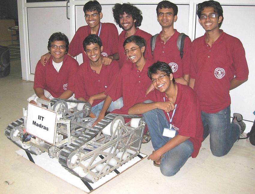
6.2.3. Final design
To troubleshoot all these problems we decided to drop this design and go ahead with a robot consisting of a
trapezoidal track belt mechanism for locomotion, somewhat similar to the kind used in tanks.
We then made a prototype based on this design for the proof of concept and tested it over various terrains,
the results were quite impressive.
• The trapezoidal tank type design gave us sufficient ground clearance
Though the robot still had problems traversing over sand. To tackle the sand issue we ordered for
high torque motors. The torque requirements are about 300kgcm and 150rpm per motor for a two
wheel drive.
Front wheel differential drive mechanism was used.
11 | P a g e• For performance on sand and gravel, we needed new track belts and wheels. Hence we outsourced
customized track belts from China for better gripping and ease of climbing over stairs.
Figure 10: Prototype 2 - CAD Front View
Figure 11: Prototype 2 – Fabricated Isometric (L) & Side View (R)
Figure 12: Final bot CAD model (w/o timing belts)
12 | P a g eThe overall assembly of the robot was split into two modules namely,
Side wheel-track belt assembly
Main Chassis
6.2.3.1. Side wheel-track belt assembly
Figure 13: Side Wheel-Track Belt Assembly
Each side of the assembly had two 4mm thick aluminium sheets attached on its outer and inner sides. The
sheets had an intricately designed and calculated truss system. The truss system gave an efficient load
distribution, increasing robustness and also reduced the weight. This truss system was cut by Plasma cutting.
In solid works 2010 we ran a simulation of this side frame structure; we put forces at the points of contact
and obtained a very satisfactory result, though some changes were made based on the results of the
simulation. For this operation the CAD diagram of the structure was given to a company “M/s. SVP laser”.
The laser sheet metal cutting machine in the “Ranganathan Building” (Manufacturing Engineering Section) in
our campus couldn’t be used as aluminium is a reflecting surface and hence the laser would reflect back and
damage the machine.
13 | P a g eFigure 14: Side Aluminium Sheet Truss System Cad
Figure 15: Side Aluminium Sheet Truss System Cad- Deformation Simulation
The Lucas TVS Wiper motor (300kgcm) was used for the locomotion. The motor shaft was just 1cm. We
couldn’t go ahead with the conventional motor flange coupling (using grub screws to attach the flange)
hence we got the small stainless steel flange welded to this shaft. This flange was attached to another long
aluminium flange by 6 nos., 5mm bolts. This technique is used to attach the cars axle with its wheels, the
reliability of this technique was much higher than the conventional one, which couldn’t bear the torque
acting (there was relative slipping between the grub screws and the stainless steel flange). This long flange
was supported by a bearing hub assembly on both sides of the aluminium sheet.
14 | P a g eFigure 16: Attachment of Motor to Aluminium Flange (Observe the welded motor shaft and the 5mm nut & bolt
attachment)
Figure 17: Long Aluminium Flange Supported by Bearing Hub Assembly on Both sides
In between these two aluminium sheets there were a total of 9 Polypropylene wheels, out of which one
geared wheel was the driving wheel (attached to the motor), another geared wheel was an idler, another
geared wheel was fixed on the rear, one large free roller wheel was fixed midway these aluminium truss
15 | P a g esystems on the leading edge of this assembly (which was useful for stair climbing) and a set of 5 free rollers
were fixed at the bottom of the arrangement for more contact points and to prevent slacking of the belt.
The idler was used to adjust the tension in the timing belt. This was done by shifting the idler
upwards/downwards in a slot using a long bolt and nut. All these wheels were manufactured in “M/s. Prem
gears” and final holes drillings (to reduce weight) was done at Velachery Lathe workshops.
A rubber synthetic polymer timing belt ran over all these set of wheels. The tension was kept medium. The
belts were partially custom made. The ones existing in the market had teeth only on one side. We stuck
rubber strips on the outer plain surface. These outer rubber treads provided us with traction and were very
vital for stair climbing.
Figure 18: Final Bot – Calculation of Track Belt Length
Figure 19: Inner and Outer Toothed Track Belt
16 | P a g eFigure 20: Adjustment Slot Mechanism of Tension in Track Belt
6.2.3.2. Main chassis:
The Main Chassis has compartments made for all the components. We had slots made for the laptop, lead
acid batteries, 5 ultrasonic sensors, camera, GPS and other circuitry. Though the chassis had only the laptop,
batteries and the motors the other components were mounted on a vertical structure which was attached to
the chassis.
Height of chassis could be adjusted according to desired ground clearance. Also the chassis could be moved
horizontally ahead/behind with respect to the robot as it was fastened with uniform holes drilled on its
edges, which were used to attach it to the Side wheel-track belt assembly.
Figure 21: Compartments for various Components on the Chassis
17 | P a g eFigure 22: Top view of the Robot with various Components
6.2.3.3. Design Verification
• After running a simulation(stress analysis) of the full robot on solid works 2010 we found out that
the weight of the robot is 35 kg
• To find out the torque requirement of the motor we ran another simulation estimating the forces
and the surface conditions
• We used DC geared motors (Lucas TVS wiper motors) of 300 kg.cm for our locomotion
6.2.3.4. Specifications
• Robot dimensions:- 850mm x 800mm x 500mm (length x width x height)
• Customized rubber polymer timing belts of 8mm pitch, 2105 mm length, 65mm width
• Frame is fabricated from 4mm aluminium sheets
• Polypropylene custom made wheels and rollers
• Powered by 24V lead acid battery
6.2.3.5. Design Strengths
• Massive customization, modular design
• 3 individual modules which are fastened together, thus giving us flexibility in size and design of the
chassis
• Any part could be modified or replaced in a short span of time
• Ground clearance of 13 cm
• Width of side-frames could be adjusted accordingly by small modifications
• Height and leading angle were designed to climb stairs
• Center of gravity was kept low for greater stability
• Tension in the belts could be adjusted by changing the height of the top idler
• Differential drive locomotion helped us to take pivot turns
18 | P a g eFigure 23: Ground Clearance
6.3. ALTERBOT - Electrical Module
6.3.1. First Algorithm development
The algorithm we thought of running integrates the data from four different high-level sensors – a GPS
navigation system, a digital compass, a LIDAR, and a camera – along with low-level sensors – four speed
encoders and a position encoder.
Data extracted from the sensors was expected to be in the following formats:
GPS: We would get a set of latitude and longitude co-ordinates in the NMEA format.
Digital Compass: It returns an Analog output that could be translated into the azimuthal angle that it is
facing w.r.t. the magnetic field of the earth. It also has a tilt sensor that detects.
LIDAR: It returns the distance of the closest obstacle at each angle in its plane of sweep. It normally
returns values for 180 - 270 degrees.
Camera: It returns a single-frame image each time it is queried, giving a colour distribution of all points
within its field of view.
Our data handling in iteration was expected to run in the following method:
We expected to run our path planning algorithm on two levels – a macroscopic level and a
micromanagement level.
19 | P a g e6.3.1.1. Macroscopic Level
We begin by obtaining the GPS coordinates of the current position of the bot. This is compared with the
GPS coordinates of the next pre-set waypoint to find distance from the waypoint and the required
heading. This heading is compared with our current heading obtained from the compass to find our
required relative heading. This information is relayed to the micro level for further processing.
6.3.1.2. Micromanagement Level
We run our image processing algorithm at this point. First, we run the image through a transformation
matrix in order to convert the image from a perspective to orthographic view. The advantage of this is
that we can now directly get an idea of the distances and angles on this transformed image. Next, the
image is run through several levels of filters (such as erode, dilate and blur) to remove any noise and to
smoothen the image. Now we run the Ground Colour Extraction algorithm to find any non-ground
objects, which are treated as obstacles. (The average value of a small square directly in front of the bot is
taken as the reference ground value, and any pixels in the whole image that match this reference are
made black. Whatever remains are ‘non-ground’ objects or regions, which are marked white). Note that
the lane boundary will also be treated as an obstacle here. We also convert the input from the LIDAR
into a 2D map of the region directly in front of us. These two inputs are now run through the following
conditions:
If the LIDAR shows a straight line and the camera shows a large continuous obstacle region, then
it means we have reached the stairs, and : 1). Required heading is set to make the bot
perpendicular to the line on the LIDAR, 2). The bot is made to run the Staircase segment of the
code.
If LIDAR shows open region and the reference of ground extraction algorithm matches a pre-set
green colour, then we run the Grass (angled tread) section of code.
If the ground reference is not green, then it is made to run Tank section (implies the vehicle is
traversing on sand or gravel)
6.3.1.2.1. Tank Mode
This mode is used when the bot is on rough terrain, for maximum stability, traction and suspension
characteristics. The paddle is raised a few degrees above the horizontal plane so it is no longer in
contact with the ground. We check the LIDAR map and the Camera map (for lane) through a filter
that gives weights to each path based on the required relative angle, which also checks for enough
space to be present for the bot to move and a minimum distance of around 50 cm. If an angle is
found based on these conditions, then this angle is set as the new heading for the bot to align to.
This is transferred to the motor-driver circuit, and the bot moves a little further forward before
running the path iteration again.
6.3.1.2.2. Grass Mode
This mode runs the same as Tank Mode, except that the paddle is lowered to around 15 degrees
below the horizontal plane first. This means that the bot is supported on four points of the treads,
which increases efficiency on flat solid ground. The motor driver also runs a different turning
mechanism to compensate for the different wheel structure.
6.3.1.2.3. Staircase Mode
This mode is run when we find a staircase in front of us. It begins just before we enter the stairs. The
paddle is raised by X degrees and the bot moves forward. On coming in contact with the stair, the
paddle will pull the front upward. This will give a major deviation on the tilt sensor of the digital
compass. The bot will keep moving forward and crossing the stairs, and during this period, we stop
taking inputs from the sensors except the tilt sensor. When the tilt sensor reading goes back to
20 | P a g enormal, it indicates that the bot is on level ground again, at which it switches out of Staircase Mode
and starts running Tank Mode again after reactivating the sensor inputs.
During all these processes, we would be using PID to make sure the bot is moving at a constant
speed on each type of terrain. (Grass – high speed, Tank – moderate, Staircase – moderate-slow)
6.3.2. Second Algorithm development
Figure 24: Processing block-diagram
The tasks that the bot should be able to accomplish to traverse the entire track are:
Lane detection
Obstacle detection
GPS based waypoint tracking
Motion planning
Processing
Integration
The control of the vehicle is done using the processing unit (Gumstix / laptop) which is placed within the
vehicle itself.
The GPS module would find out the current coordinate of the vehicle and based on the coordinates of the
next waypoint it decided the direction in which the vehicle should head. The digital compass gives the
current orientation of the vehicle. It helps in keeping the vehicle on track towards the next waypoint. The tilt
21 | P a g esensors inbuilt into the digital compass helped to plan the next motion based on the tilt of the vehicle with
respect to the ground. This particularly helped during climbing stairs and slopes.
A LIDAR scanning module was expected to be used for profiling the environment and detecting the modules.
This was preferred over using an array of ultrasonic sensors as used in iCar as the environment was more
cluttered as this is an off-road terrain and we needed a greater view angle with high resolution for making
efficient decisions. Moreover the overall cycle-speed of the LIDAR was much faster than an array of
ultrasonic sensors.
E-Stop – The vehicle was equipped with both manual and wireless E-stops. When either E-stop is engaged
an abort signal stopped the execution of the controller program and turned off the control signal to the
motor drivers. Additionally, mechanical relays could also be used, which would disconnect the motor power
wiring from the amplifiers and apply a regenerative power dissipation resistor across the motor leads, which
would help slow the vehicle to a quick stop.
6.3.2.1. Lane detection
Figure 25: Position of Web Camera on the Robot
In our project the main aim of image processing is for achieving two objectives:
Lane detection – to detect the end lanes of the road, thereby keeping the car on the road at all
times.
Obstacle Detection – to aid the ultrasonic module with the obstacle avoidance.
We used the C language with the OpenCV Package for all our Image Processing work.
The following steps were taken to achieve the objective:
6.3.2.1.1. Image Plane Transformation
This is a process used to convert the 2D perspective output of the camera into a more informative
orthographic view. This is based on the assumption that the surface of the road is a perfect plane in
front of the camera.
Each point in 3D has (X, Y, Z) coordinates and that is transformed to (x, y), i.e. the 2D pixel coordinates by
the formula:
Where is the focal length.
22 | P a g eThus the 3D plane of the road, the Ground Plane is rotated to a vertical plane, the Orthogonal Plane.
Equation of the ground plane:
Equation of the orthogonal plane:
Figure 26: Schematic of the ground and the orthogonal planes
In the image of the ground plane let the point P corresponding to pixels P get transformed to the
pixel Q . Then, there exists a transformation matrix H such that:
Where, [ ]
The transformation equation can also be written as:
[ ] [ ][ ]
By solving and normalizing for z coordinate for any 4 points (P1,P2,P3,P4) given that we can find the
coordinates of (Q1,Q2,Q3,Q4) by some other means, we can obtain all the 8 unknowns of the H matrix.
We can derive the H matrix from the perspective image if we know the focal length.
The H matrix depends on the camera, the orientation and the height of the camera above the ground.
Once found out, it becomes a characteristic of that configuration and can then be applied to any image
taken by the camera.
Since we were working with a webcam the actual focal length of the camera was not available.
Therefore we had to make calculated guesses as to what the points Pi would correspond to in the
orthogonal image. Thus, the points Qi were guessed by us.
To find H
By using equation (1), for each transformation of P → Q we get the following two normalized equations:
23 | P a g eThus, we get 2 equations for 1 point. With 4 points we’ll get 8 equations.
Now, these equations can be rewritten as:
We can solve these 8 equations for a1, a2, a3, b1, b2, b3, c1, c2 simultaneously by collecting all the
coefficients on the left hand side as an 8X8 matrix A. The unknown matrix X is an 8X1 column matrix of
the unknowns. The RHS forms an 8X1 column matrix B of the values x’ and y’ of 4 points.
Thus we get,
Rearranging the entities in X in a 3X3 form we get the H matrix.
Apply this H to get the orthogonal image from the perspective image
We applied this H to all the pixels in a perspective image. We have to check that if the transformed
coordinates fall outside the limits of the image we must not consider them. Also as the transformed
coordinates come out to be fractions we round them to integers. If we get a valid transformed
coordinate, then copy the RGB values of the original coordinate into this coordinate.
When we did this we found that as this process eliminates a lot of coordinates by expanding the image,
the resulting image had large patches of undefined pixels.
Thus we worked backwards:
The transformation is:
Thus,
For each pixel in the result image, scan in the original image if a corresponding pixel exists. If it does,
then copy the RGB streams of the pixel.
This has the benefit that each pixel in the resultant image scans if a valid corresponding pixel is there in
the original image. Thus the holes are minimized and we get a much better result image.
Image quality can be further improved by taking the values from a kernel around the targeted pixel and
using various interpolation techniques. This reduces the stark contrasts and noise commonly otherwise
found in the resultant image.
The resultant image now is an orthogonal top view of the road directly in front of the bot. This allows to
easily measure distances between objects in front of the bot, as all angles between points measured on
this image are equal to their corresponding points in real life. Also, the pixel-distance between points on
24 | P a g ethe image is directly proportional to the real distances between these same points. This essentially gives
us a scaled map of the region directly in front of the bot.
Figure 27: Perspective View (Day – Light) Figure 28: Transformed View (Day-Light
Figure 29: Perspective View (sodium vapour light) Figure 30: Transformed View (sodium vapour light)
Figure 31: Perspective view (DRDO view) Figure 32: Transformed View (DRDO venue)
6.3.2.1.2. Colour Detection and Ground Extraction
For extracting the colours, we had to use a system of colour detection that was reliable and independent
of lighting conditions, which could not be done in the standard RGB (Red-Green-Blue) colour-space.
Instead, we converted the image into the HSV colour-space, which generally has much better results in
terms of comparing colours and being light-independent. HSV stands for Hue-Saturation-Value, and
represent a set of three independent variables that can be used to represent human visual perception of
colour much better than the RGB method. The Hue value here is a value between 0 and 180, and loops
back (H=0 is identical to H=180), and represents the general position of the colour on the colour
25 | P a g espectrum. Saturation represents the amount of colour present, with low values of saturation appearing
to be bleak, monochrome images. The value of S ranges from 0 to 255. The Value represents the amount
of lighting, with lower Values showing higher amounts of black and higher Values corresponding to
brighter images. Value also ranges from 0 to 255. This type of distribution means that a single value of
hue can be used to represent a single perceived colour and that only the Value will change with change
in lighting. When comparing a pixel’s HSV values with the template, we checked to see whether the test
pixels values of H and S were within a set interval of the template’s H and S values. V was neglected as
we had no use for checking the lighting conditions. We found that an interval of about 10 units around
the reference H value, and about 50 around S worked best for our purposes.
The next step after this is finding useful points of data from the image, which are essentially the lane
boundaries. As an added bonus, if obstacles can also be detected, an accurate map of their positions can
also be plotted thanks to the Image Plane Transformation. Hence, instead of directly looking for the lane
boundaries in the image (which were marked in yellow dashes), we chose to use a method called
Ground Extraction.
The concept of ground extraction is to look within the image for traversable ground, and identify
everything that does not correspond to the ground to be classified as an obstacle. In other words, we
compare every pixel in the image with a pre-existing template of the ground. If the values match, then
that pixel is identified as a ground pixel. If they do not match, then an obstacle is identified at that point.
In this way, we binarize the image such that every pixel occupies one of two states – ground or non-
ground. The non-ground areas are treated as obstacles and are meant to be fed into the data for
obstacle detection from the ultrasonic sensor array. This allows the image-processing code to
complement the obstacle-detection code. Coincidentally, the lanes are also detected as obstacles in this
process, so the lane-following algorithm is combined with the obstacle-detection code. Here, we
consider the lanes as an obstacle, rather than as lines that we need to align the bot to.
However, the problem statement involved the bot having to go over several types of terrain. This meant
that we could not use a single template for the ground-extraction process. Also, a standardised set of
templates was more likely to fail us, either by not being able to detect intermediate areas of ground or
falsely detecting ground in case we had too many templates. Hence, we chose to use a constantly-
adapting template selection method based on the assumption that the initial obstacle-detection code
works and that no obstacle will ever come near the front of the bot. As long as we know that there is
clear open ground in front of the bot, we take the template as a sample from the bottom-centre of our
image (which corresponds to the area immediately in front of the bot). In this way, the AI will
automatically try to keep the bot following whatever surface it is currently on.
26 | P a g e6.3.2.1.3. Edge Detection and Lane Adjustment
Figure 33: Prototype for testing Lane Detection
Along with feeding the obstacle data into the obstacle-avoidance code, we also executed a parallel lane-
finding code by looking for and extracting only the yellow lines within the image. Once the lanes had
been detected and moved into a separate binary image, we first ran them through an edge-detection
function (cvCanny()) to find the edges of the lane patches. In case of noise-filled images where a clear
line was not visible in the edges, we increased the thickness of the lines to compensate for this.
After the edge detection, we ran the resulting image through a Hough Transform filter, which was
another pre-defined OpenCV function (cvHoughLines2()). The Hough Lines works on the principle of
finding lines using the parametric equation of lines:
For every pixel, the code makes a note of all the possible and values of that pixel. After scanning the
entire image, it checks to find the ( , ) pairs that got more that a certain number of hits. These are the
lines identified by the function, and it outputs the ( , ) values of each such detected line.
We calibrated this HoughLines code to find only the edges of the lanes, which gave us the alignment of
the lanes, as well as their distance from the bot. Using this data; we got information about the alignment
of the bot with respect to the lanes.
Incidentally, it was noticed that during all test conditions, due to restrictions on the observable area of
the camera, we never had more than one lane in view at any time. Hence we optimized the control code
at these times to align the bot such that its main axis was tangential to the lane, and obstacle detection
was given lower preference, only alerting the program when an obstacle was detected close to the bot.
This allowed for fast travel in a single direction. During instances of multiple or zero lane detections, we
reverted to our original path-finding code based on the obstacle-avoidance algorithms, which gave a
slower, more accurate response.
27 | P a g eFigure 34: Original Filtered Image Figure 35: Image Processing Result
Create a binary Apply Canny filter
Load image from
image of only to binary to find
camera
found lanes edges
Thicken the edges
Image plane Scan for and find
to compensate for
transformation yellow areas
noisy lanes
Convert image Use HoughLines to
Erode filter to
from RGB to HSV define edges of
reduce noise
color space lanes
Figure 36: Final Lane Detection Algorithm Flowchart
6.3.2.2. Obstacle detection
6.3.2.2.1. Components
6.3.2.2.1.1. LIDAR: (initial component)
Output of the LIDAR is a part of obstacle detection algorithm. LIDAR is a laser based 2D
range scanner.
It gives a polar profile of the distance of the nearest obstacle in that angle based on its
angular resolution.
The LIDAR that we intended to use is URG-04LX-UG01.
o range - 5.6m
o accuracy - +/- 30mm
o frequency - 10Hz
o Angular resolution - 0.36 deg.
28 | P a g eWe had the algorithms for obstacle avoidance ready. But, unfortunately the LIDAR broke
down and was not functional and hence we had to send it for repair. In the meanwhile we
explored the option of using ultrasonic sensors for navigation.
6.3.2.2.1.2. ULTRASONIC SENSORS: (Finally used component)
Maxsonar EZ1 and WR1
6.25m range, narrow beam
6.3.2.2.2. Initial Obstacle Avoidance Algorithm
Of the many obstacle avoidance algorithms we looked through, we found the Vector Field Histogram
(VFH), by J. Borenstein and Y. Koren, a good starting point for us. The reason was that while there
were some algorithms which were not processor intensive, their assumptions were based on the
fact that the path being traversed is an open path. This assumption frees the algorithm from the
rigors of cluttered environments as the path is an open one and one did not necessarily need an
optimum path or a preordained direction.
Of the closed path algorithms, we found that the VFH approach exerted lesser load than most of the
other codes. Also, it could be used for fast moving robots.
The original code used by us in iCar was similar to the VFH* approach which was an improvement
over the original VFH by Iwan Ulrich and Johann Borenstein. However, this approach was very slow,
thus we decided to derive it from the VFH itself.
One of the salient features of the VFH approach is that it takes into account the possibility of
erroneous readings due to noise and counters it with fast sampling. A cumulative addition of data
acquired over many samples helps us assigning a certainty value to each cell which is proportional to
the probability of an obstacle being there. These certainty values are used to make a polar histogram
which gives us the urgency of obstacle avoidance in each direction.
A certain threshold value for the histogram can be selected and all the valleys in the histogram
below this threshold are good candidates for the next step. These candidates are compared on the
grounds of width and proximity to target direction and a decision is taken.
Also, the algorithm uses a smoothing function for the histogram which makes sure that the bot does
not take abrupt turns.
And more importantly, the algorithm works very well for narrow paths and cluttered environments.
We can also assign it speed as a function of the direction being taken and the response of the
histogram in that direction and the maximum speed in that particular terrain.
However, one difficulty in the algorithm is that it requires the maintenance of a moving active
window and obstacles in this window are the only ones considered for the algorithm. Keeping a track
of such a window and can be tricky as it depends on the feedback from optical encoders and a digital
compass. However, under sufficiently controlled speeds and decent assumptions, this can be done.
Although the algorithm is for local obstacle avoidance, with the help of a bounded path and target
coordinates, the result can be very close to an optimum path and can help our bot to move through
all the obstacles with decent speed and accuracy.
However, for our requirements, even these algorithms turned out to be too slow to be implemented
with practical speeds with the processing power we had. Thus we finally ended up using an
29 | P a g ealgorithm which assumed the polar space to be divided into 6 segments and the bot had the option
to move within these based on a weighted function we decided which took the readings from the
ultrasonic sensors for the respective segments as inputs.
6.3.2.2.3. Final Obstacle Avoidance Algorithm
All sensors are flagged to be Saturation Limits for the
taken into account for decision individual sensors are applied
wherever applicable
Sensor readings below a lower
cap are ignored by flagging those
Path decision - only high flagged
sensors low. This later helps as
sensors’ data is considered.
we dont have to keep track of
each sensor value.
The direction for the largest
obstacle free distance is the
output. The distances are scaled
The robot moves in this direction
according to weightages which
tell us about the critical direcions
and thus also critical obstacles.
Figure 37: Final obstacle avoidance algorithm
Criticalities:
As it was difficult to accurately ascertain about obstacles that were farther than about
4m, we set a saturation limit for each sensor output. This made avoiding side grazes
easier.
These readings were averaged to reduce noise.
However, averaging was not enough and it gave bumpy results. As we were using analog
output, we could use analog filters to smoothen the output.
The sensor angles and the weightage functions were placed such that taking turns also
assured that no other part of the body was grazing with any obstacle.
30 | P a g eFigure 38: Position of Ultrasonic Sensors on the Robot
6.3.2.2.4. Ultra Sonic Sensors Used
As can be seen from the picture above, we used two types of ultrasonic sensors. They were
MaxSonar EZ1(qty=1) and MaxSonar WR1(qty=4).
Max Sonar EZ1
Datasheet Link
Max Sonar WR1
Datasheet Link
As one can see from the datasheet, EZ1s are cheaper than WR1s. This is because WR1 can give a
much more narrow cone angle (the actual locus is not that of a cone though) than the EZ1. Also the
PVC covering gives it a better protection against dust. Due to the size of our bot and its relative size
to the obstacles being the same (or of lower order), we decided that the front sensor could just give
us an output based on whether an obstacle is there straight ahead. Thus we kept a wider angle EZ1
sensor in the front. To WR1s were kept at a similar (slightly tilted) angle so that the entire front
portion could be mapped and also some information on the size of the obstacle could be
determined. This would help us in taking an imminent diversions (for example to over-take) at a
much earlier time and thus at a much smoother angle. The sideways oriented sensors (extreme
right and left WR1s) apart from giving data about obstacles at the side which would help us taking
smoother turns in wide roads, also gave us the manoeuvrability while taking tight turns. As the data
quality had to be high for taking proper safe tight turns, we took the narrow angled WR1 sensors
which increased the resolution at the sides where higher chances of scraping can be seen.
31 | P a g eThe output taken from both these types of sensors was of the Analog form as it is easier to process.
It would be wise for one to use Analog filters as it greatly reduces the noise. To get an Analog
reading there are two ways, you continuously get readings where the ultrasonic pulses are kept on
being sent at a fixed safe delay decided by the manufacturer or we send pulses only when we want
to but sending a high to the Rx Pin for greater than 20 µsec. We used the second method as we had
many sensors acting together and simultaneous firing may give wrong results as pulse of one sensor
may be detected by the other. So one has to fire the sensors in a chain sequence. These chain
algorithms can be autonomously or processor controlled. We controlled the firing sequence with the
micro controller as this way one can be assured that we don’t get out-dated results. These chain
algorithms (if to be fired in a fixed time cycle) can be found in the sensor FAQ link.
Reading these Analog values is in our case was done by the Arduino Mega which has a pretty easy
and helpful library. Our initial prototype had used an AtMega 16 to read these. These values were
converted to digital form by the ADC units of the respective controllers to which a particular scaling
constant would have to be multiplied to get the required distance.
6.3.2.3. GPS based waypoint tracking
6.3.2.3.1. GPS receiver
The main task of this unit is to detect the present position of the robot in terms of its latitude and
longitude.
These values are compared with the next GPS waypoint provided so that the robot can be directed
towards the next waypoint based on the heading calculated. There were totally 30 GPS waypoints that
had to be reached.
The algorithm for the calculation of heading is as follows:
The GPS units follow NMEA format for transfer of data in the form of sentences. We read each
of the sentences completely to ensure that no data is lost. We store the sentences which start
with the word GPGGA as these sentences contain the information on latitude and longitude.
We then read the latitude and longitude, which are in ASCII format and convert them to latitude
and longitude in degrees. A sample GPGGA statement is given as follows:
$GPGGA,123519,4807.038,N,01131.000,E,1,08,0.9,545.4,M,46.9,M,,*47
Where:
o GGA: Global Positioning System Fix Data
o 123519: Fix taken at 12:35:19 UTC
o 4807.038,N: Latitude 48 deg 07.038' N
o 01131.000,E: Longitude 11 deg 31.000' E
o 1 : Fix quality:
0 = invalid
1 = GPS fix (SPS)
2 = DGPS fix
3 = PPS fix
4 = Real Time Kinematic
5 = Float RTK
6 = estimated (dead reckoning) (2.3 feature)
7 = Manual input mode
32 | P a g e 8 = Simulation mode
o 08 : Number of satellites being tracked
o 0.9 : Horizontal dilution of position
o 545.4,M : Altitude, Meters, above mean sea level
o 46.9,M : Height of geoid (mean sea level) above WGS84 ellipsoid
o (empty field) : time in seconds since last DGPS update
o (empty field) : DGPS station ID number
o *47 : the checksum data, always begins with *
Once we convert latitude and longitude into the required format we compare it with the next
waypoint and get the required heading by using the ‘Haversine’ formula.
Where,
All the parameters in this formula should be given in radians. The result that comes out is also in
radians.
We follow this heading and keep checking the GPS coordinates after each fixed interval (based
on speed of robot) and identify when we reach the required waypoint.
The information on the current heading of the robot is obtained using a digital compass. In this
case we used a digital compass from Microstrain (3DM – GX1) which gives current heading on
enquiry.
Based on this heading information we align the robot to the calculated heading. However the
code is such that the robot gets aligned only if it does not see any obstacles and the lane. If
either of them is seen then they get priority and the robot heads in the required direction. If
there is no obstacle or lane then the robot travels in the direction of the calculated heading.
Once we reach the required waypoint we head towards the next waypoint.
We used the San Jose navigation GPS.
32 channel
Accuracy - 3.3 m
Selectable update rate from 1 - 5 Hz
Follows NMEA standards
Figure 40: GPS module Used Figure 39: Microstrain module used
6.3.2.3.2. Digital Compass
We used a digital compass to detect the current heading of the bot and also the inclination of the bot. It
helped us to align the robot towards the next way point after it had reached the previous waypoint.
33 | P a g eWe needed the inclination of the bot so that we could have better control over the bot and to help us
while climbing stairs.
The digital compass which we used was 3DM-GX1 (Gyro Enhanced Orientation Sensor):-
Three axis of magneto, three axis of accelerometer, and a PIC core running all the calculations.
On-board processing/filtering of accelerometer, gyro and magnetometer output
Fully compensated over wide temperature range
Outputs Euler angles, quaternion, orientation matrix, attitude and heading (azimuth/yaw) or raw
sensor data
Standard RS-232, RS-485 outputs, optional analog output
6.3.2.3.3. Interfacing GPS and the Digital compass
We coded the algorithm for effective point to point navigation and implemented it on our test bot. The
GPS and the digital compass data were received from the sensors by using Serial port communication
through USB ports.
6.3.2.3.4. Final GPS Navigation Algorithm Flowchart
Detect current GPS
waypoint.
Find the heading of the next
Make new measurements w.r.t
waypoint based on current GPS
next waypoint
waypoint (Haversine formula)
Align the bot to the required
Update that the GPS waypoint heading by detecting the current
has been reached heading of the bot.
Traverse to the required waypoint
along with avoiding the obstacles
on it’s way.
Figure 41: GPS navigation algorithm
6.3.2.3.5. Challenges in GPS
Problem: Due to the low update rate of GPS compared to the speeds of other sensors, time lag
in code.
Solution: Used some properties of buffer memory to use GPS data only when it is received
completely.
Problem: Alignment of the robot with the required heading angle was difficult when we did
bang- bang control.
Solution: Used proportional control for turning the bot.
34 | P a g eYou can also read