Impact of Lagrangian transport on lower-stratospheric transport timescales in a climate model
←
→
Page content transcription
If your browser does not render page correctly, please read the page content below
Atmos. Chem. Phys., 20, 15227–15245, 2020
https://doi.org/10.5194/acp-20-15227-2020
© Author(s) 2020. This work is distributed under
the Creative Commons Attribution 4.0 License.

Impact of Lagrangian transport on lower-stratospheric transport
timescales in a climate model
Edward J. Charlesworth1 , Ann-Kristin Dugstad1 , Frauke Fritsch2 , Patrick Jöckel2 , and Felix Plöger1,3
1 Forschungszentrum   Jülich, IEK-7 Stratosphäre, Jülich, Germany
2 Deutsches   Zentrum für Luft- und Raumfahrt, Institut für Physik der Atmosphäre, Oberpfaffenhofen, Germany
3 Institut für Atmosphären- und Umweltforschung, Universität Wuppertal, Wuppertal, Germany

Correspondence: Edward J. Charlesworth (edward.charlesworth.science@gmail.com)

Received: 11 May 2020 – Discussion started: 9 July 2020
Revised: 2 October 2020 – Accepted: 20 October 2020 – Published: 8 December 2020

Abstract. We investigate the impact of model trace gas trans-         tropopause transport in EMAC. Potential consequences from
port schemes on the representation of transport processes in          the choice of the transport scheme on chemistry–climate and
the upper troposphere and lower stratosphere. Towards this            geoengineering simulations are discussed.
end, the Chemical Lagrangian Model of the Stratosphere
(CLaMS) was coupled to the ECHAM/MESSy Atmospheric
Chemistry (EMAC) model and results from the two transport
schemes (Lagrangian critical Lyapunov scheme and flux-                1   Introduction
form semi-Lagrangian, respectively) were compared. Advec-
tion in CLaMS was driven by the EMAC simulation winds,                The upper troposphere and lower stratosphere (UTLS) is an
and thereby the only differences in transport between the             important region for global climate as the chemical compo-
two sets of results were caused by differences in the trans-          sition of radiatively active trace gas species there has crucial
port schemes. To analyze the timescales of large-scale trans-         impacts on radiation and surface temperatures (e.g., Solomon
port, multiple tropical-surface-emitted tracer pulses were            et al., 2010). The entry of air masses into the stratosphere is
performed to calculate age of air spectra, while smaller-scale        controlled by the chemical and dynamical processes in the
transport was analyzed via idealized, radioactively decaying          UTLS (e.g., Holton et al., 1995; Fueglistaler et al., 2009),
tracers emitted in smaller regions (nine grid cells) within the       presenting a challenge for understanding and modeling the
stratosphere. The results show that stratospheric transport           region. To overcome, climate models must have a realistic
barriers are significantly stronger for Lagrangian EMAC-              representation of UTLS transport processes in order to pro-
CLaMS transport due to reduced numerical diffusion. In par-           vide reliable predictions and assist in robust theoretical de-
ticular, stronger tracer gradients emerge around the polar vor-       velopment. For instance, in simulating the effects of geoengi-
tex, at the subtropical jets, and at the edge of the tropical pipe.   neering by sulfur injections into the stratosphere, uncertain-
Inside the polar vortex, the more diffusive EMAC flux-form            ties in the model transport representation could cause sub-
semi-Lagrangian transport scheme results in a substantially           stantial uncertainties in the simulations (Tilmes et al., 2018;
higher amount of air with ages from 0 to 2 years (up to a             Kravitz and Douglas, 2020). Even small differences in com-
factor of 5 higher). In the lowermost stratosphere, mean age          position caused by model differences in small-scale trans-
of air is much smaller in EMAC, owing to stronger diffu-              port processes (e.g., turbulence, diffusion) may cause signif-
sive cross-tropopause transport. Conversely, EMAC-CLaMS               icant model spread in surface temperatures (e.g., Riese et al.,
shows a summertime lowermost stratosphere age inversion –             2012). This radiative effect of composition changes in the
a layer of older air residing below younger air (an “eave”).          UTLS is particularly large for water vapor but also substan-
This pattern is caused by strong poleward transport above             tial for other species like O3 , N2 O, and CH4 .
the subtropical jet and is entirely blurred by diffusive cross-          Critical processes for models are transport around the win-
                                                                      tertime stratospheric polar vortex, stratosphere–troposphere

Published by Copernicus Publications on behalf of the European Geosciences Union.
15228                     E. J. Charlesworth et al.: Lagrangian vs. Eulerian transport: investigation through age spectra

exchange across the tropopause, and horizontal exchange            from each other when no inter-parcel mixing scheme is ap-
between the tropical lower stratosphere (the tropical pipe;        plied. Parcel mixing due to small-scale processes (e.g., tur-
Plumb, 1996) and middle latitudes (for reviews of strato-          bulence) can then be introduced based on physical param-
spheric transport processes see e.g., Plumb, 2002; Shepherd,       eterizations, and the strength of mixing can then be con-
2007). The steep gradients in observed trace gas distributions     trolled. Due to the complications of handling irregular (air
in these regions are signs of transport barriers and regions       parcel) grids, Lagrangian schemes are not commonly used
of suppressed exchange, for example, around the polar vor-         in global climate models. To our knowledge, the only two
tex, at the edge of the tropical pipe, and along the extratrop-    Lagrangian transport schemes which are currently imple-
ical tropopause. The representation of transport processes in      mented in a global climate model are ATTILA (Stenke et al.,
the lower stratosphere in global models is prone to numerical      2008, 2009; Brinkop and Jöckel, 2019) and CLaMS (Hoppe
diffusion, as tracer distributions in this region are character-   et al., 2014, 2016). Both these schemes have been integrated
ized by sharp gradients and frequent small-scale filamentary       into the ECHAM/MESSy Atmospheric Chemistry (EMAC)
structures (McKenna et al., 2002).                                 climate model (e.g., Jöckel et al., 2005, 2016), and at the
   Atmospheric models (as used in current coupled                  present time neither has been incorporated into another cli-
chemistry–climate models) employ different numerical               mate model.
schemes for solving trace gas transport, all of which intro-          Stenke et al. (2008) showed that using the ATTILA
duce some unwanted, unphysical numerical diffusion. Nu-            scheme in EMAC reduced the excessive transport of water
merical diffusion smoothes gradients and small-scale fila-         vapor into the lowermost stratosphere and into polar regions,
ments in tracer distributions, and thereby differences in nu-      and the associated cold bias in temperatures could be partly
merical diffusion cause differences in trace gas transport         corrected. The representation of stratospheric ozone was also
in different models, affecting the simulated distributions of      found to have been improved (Stenke et al., 2009). Hoppe
trace gas species. Research has been focused on this topic for     et al. (2014) further showed that CLaMS transport within
decades, with early work performed by Rood (1987) for one-         EMAC results in a more realistic representation of transport
dimensional flow. Numerical diffusion in multi-dimensional         barriers around the southern polar vortex, due to reduced nu-
models, using mean age of air as a diagnostic, was studied         merical diffusion compared to the EMAC-FFSL scheme.
by both Hall et al. (1999) and Eluszkiewicz et al. (2000),            Here, we build on the study of Hoppe et al. (2014) and fur-
while Gregory and West (2002) performed a similar study fo-        ther analyze the implementation of the Lagrangian transport
cusing on stratospheric water vapor transport. These studies       scheme CLaMS within the EMAC climate model. We com-
found significantly younger stratospheric mean age of air and      pare results from two tracer sets within one EMAC simula-
a faster water vapor tape recorder propagation for more dif-       tion: one set where transport is calculated using the EMAC-
fusive transport schemes. Later, Kent et al. (2014) provided a     FFSL scheme and one set using the CLaMS Lagrangian
detailed analysis of idealized tracers and transport scenarios.    tracer transport scheme. To enable a more detailed analysis
Most recently, Gupta et al. (2020) studied a variety of dy-        of composition and transport timescales, going beyond the
namical cores using mean age of air as a transport diagnos-        average stratospheric transit time (the mean age; Waugh and
tic, demonstrating that many issues with numerical diffusion       Hall, 2002) as considered by Hoppe et al. (2014), we calcu-
are still relevant with modern techniques and computational        late the full (time-dependent) stratospheric age of air spec-
resources.                                                         trum (the distribution of stratospheric transit times) of model
   Most currently used transport schemes are based on a reg-       transport schemes.
ular grid (e.g., Morgenstern et al., 2010) and will be referred       This work investigates the differences in transport in the
to as Eulerian schemes in the text to follow. Another class of     lower stratosphere between these two transport schemes us-
transport schemes, Lagrangian schemes, on the other hand,          ing the age spectrum, mean age, and idealized tracers as di-
follow the motion of air parcels through the atmospheric           agnostics. The work is focused on identifying the regions that
flow and hence have reduced diffusion characteristics due          are most sensitive to changes in the tracer transport scheme,
to the absence of interpolations of tracer distributions to a      assessing the timescales for which the transport schemes dif-
regular grid (e.g., McKenna et al., 2002). Semi-Lagrangian         fer, and identifying the potential consequences for simulated
schemes are still based on a regular grid, but they incorporate    chemical composition and geoengineering simulations.
some advantages of Lagrangian transport by calculating the            In Sect. 2 the used models and diagnostic methods (age
air motion over one model time step through a Lagrangian           spectrum, forward tracers) are introduced. Section 3 presents
advection scheme, but this is then followed by remapping           the results from a global perspective, while Sect. 4 focuses
onto the grid. One such scheme which is both sophisticated         on particular processes and regions. In Sect. 5 the transport
and frequently used in global models is the flux-form semi-        scheme differences are discussed against the background of
Lagrangian (FFSL) scheme (e.g., Lin and Rood, 1996; Lin,           current research on stratospheric geoengineering. The main
2004).                                                             conclusions are summarized in Sect. 6.
   Fully Lagrangian transport schemes, by definition, are free
of numerical diffusion, as parcels are left entirely isolated

Atmos. Chem. Phys., 20, 15227–15245, 2020                                          https://doi.org/10.5194/acp-20-15227-2020
E. J. Charlesworth et al.: Lagrangian vs. Eulerian transport: investigation through age spectra                               15229

2     Methods                                                      is a hybrid σ − θ coordinate (referred to as ζ ) (Hoppe et al.,
                                                                   2014). Above the prescribed reference pressure of 300 hPa,
2.1    Models                                                      ζ is identical to θ and therefore the vertical advection ve-
                                                                   locity throughout the stratosphere is identical to the dia-
The model used in this work is EMAC, the MESSy (Mod-               batic heating rate. CLaMS advection is normally driven by
ular Earth Submodel System) version of the ECHAM5 cli-             horizontal winds and diabatic heating rates from reanalyses
mate model (see Jöckel et al., 2010 for details on EMAC            (e.g., Konopka et al., 2007; Ploeger et al., 2019); however
and Roeckner et al., 2006 for details on ECHAM5). EMAC             in EMAC-CLaMS advection of CLaMS parcels is driven by
is a modern chemistry–climate model which is commonly              the horizontal winds and heating rates of EMAC. This advec-
used for studies of the stratosphere and upper troposphere         tion is driven online, during execution of the simulation, so
(Sinnhuber and Meul, 2015; Oberländer-Hayn et al., 2016;           that the underlying velocity fields for advection in EMAC-
Fritsch et al., 2020), as well as studies of the troposphere.      CLaMS and EMAC-FFSL are exactly the same. However,
In this work, EMAC is operated at the T42L90MA spectral            there are two differences in how these fields are used by the
resolution, corresponding to a horizontal quadratic Gaussian       transport schemes. (1) EMAC-CLaMS interpolates the hor-
grid of approximately 2.8◦ × 2.8◦ resolution with 90 ver-          izontal winds onto parcel locations, whereas EMAC-FFSL
tical layers. One simulation is performed with this model,         uses the winds directly on the EMAC grid points. (2) As
by which two sets of time-resolved tracer distributions were       mentioned above, the vertical velocity of EMAC-CLaMS
calculated. One tracer set was calculated with the standard        is the diabatic heating rate (calculated by EMAC), whereas
EMAC-FFSL transport scheme and will be referenced as the           EMAC-FFSL uses a kinematic vertical velocity (calculated
Eulerian representation or EMAC-FFSL. The other tracer set         by closure of the mass balance equation). The horizontal and
was calculated with the CLaMS EMAC submodel and will               vertical velocities in the two transport schemes are therefore
be referenced as the Lagrangian representation or EMAC-            consistent, but not actually identical. More details of EMAC-
CLaMS.                                                             CLaMS are described by Hoppe et al. (2014, 2016).
   The EMAC-FFSL transport scheme is the flux-form semi-
Lagrangian (FFSL) scheme (Lin and Rood, 1996), which is            2.2   Age spectra
used in many modern climate models. The EMAC-FFSL ver-
tical coordinate is a hybrid sigma-pressure coordinate, which      The goal of this work is examination of differences in tracer
is another common choice in the development of modern cli-         transport between two advection schemes, for which analy-
mate models. The time resolution of the EMAC simulation            sis of passive tracers is ideal. This approach, as opposed to
performed in this work is 12 min. The simulation consists          examination of chemically active species, eliminates differ-
of 10 years of spin-up, with a following 10 years of result        ences that could arise through the differing chemical schemes
production. The EMAC version used in this work is 2.53.1,          of EMAC and the CLaMS submodel of EMAC. The diag-
and the model was free-running (i.e., not forced by meteoro-       nostic tool used in this work is the age spectrum, G(r, t, τ ),
logical fields). Although EMAC can be used for chemistry–          which describes the probability distribution of stratospheric
climate model simulations, the configuration in this work          transit times τ (age) within an air parcel sampled at location
did not simulate interactive chemical fields. The water vapor      r and time t (e.g., Waugh and Hall, 2002). The first moment
field, however, was interactive, and included stratospheric        of the age spectrum is the mean age 0, which represents the
moistening via methane oxidation (see e.g., Revell et al.,         average transit time from a tracer source region to a given
2016). Sea-surface temperatures and sea ice were prescribed        point in the atmosphere
from the HadISST climatology (Rayner et al., 2003). Mean-                      Z∞
while, CO2 , CH4 , N2 O, CFC-11, and CFC-12 mixing ratios
                                                                   0(r, t) =        τ G(r, t, τ ) dτ .                           (1)
were fixed at 367 ppmv, 175 ppmv, 316 ppbv, 262 pptv, and
520 pptv, respectively, for calculation of radiation. Other de-                0
tails of the EMAC set-up are identical to those of Jöckel et al.      In models, age spectra can be calculated by a series of trac-
(2016).                                                            ers which are pulsed at some reference location (in this case
   CLaMS (the Chemical Lagrangian Model of the Strato-             the tropical surface). For such a tracer with a pulse in the
sphere) is a Lagrangian chemical transport model based on          source region at time ti the mixing ratio χ i (r, t) at point r
three-dimensional trajectories and an additional mixing pa-        and time t can be normalized to the probability density for
rameterization. The EMAC-CLaMS results in this work were           air of the transit time τ = t − ti , which is the value of the age
produced with a resolution of approximately 3 million air          spectrum.
parcels. Unique among Lagrangian models, CLaMS uses a
mixing parameterization which is robustly based on physi-          G(r, t, t − ti ) = χ i (r, t)                                 (2)
cal principles. This parameterization is based on the critical
Lyapunov exponent method, details of which can be found            Therefore, a suite of pulse tracers provides the full transit
in Konopka et al. (2004). The vertical coordinate of CLaMS         time dependency of the age spectrum function G.

https://doi.org/10.5194/acp-20-15227-2020                                           Atmos. Chem. Phys., 20, 15227–15245, 2020
15230                      E. J. Charlesworth et al.: Lagrangian vs. Eulerian transport: investigation through age spectra

   This boundary impulse response method has been used
in a few other modeling studies to calculate fully time-
                                                                                  Z∞
dependent stratospheric age spectra (for further details see          T                                  τ
e.g. Li et al., 2012; Ploeger and Birner, 2016; Hauck et al.,        χ (r, t) =        χ0T G(r, t, τ ) e− T dτ .                (3)
2019). In this work, the tracers are emitted over the course                      0
of 30 d, after which emissions are ceased, and one tracer is
pulsed every 3 months, specifically in January, April, July,         Here, χ0T is the tracer mixing ratio at the tropical surface.
and October of each year, analogous to the set-up by Hauck             Throughout this paper, this quantity will be referred to as a
et al. (2019). Tracer emission is performed by prescribing           “forward tracer”, as it is computed forward from the knowl-
the surface boundary mixing ratio in EMAC. Each tracer               edge of the age distributions throughout the model domain.
is therefore assigned an age based on when the tracer was
                                                                     2.4   The EMAC-CLaMS lower and upper boundaries
emitted, and the combined set of tracers is used to create the
age distribution. Forty tracers are utilized in total, such that     A critical decision in this study lies in the way in which age
the calculated age spectra span the course of 10 years. Af-          tracers are pulsed. Differences in the age spectra between the
ter 10 years, mixing ratios of the oldest tracer are set to zero     two transport schemes would ideally stem only from differ-
throughout the model domain and the tracer is re-pulsed, so          ences in transport within the region of interest (the strato-
that the age spectra always span from 0 to 10 years. Further-        sphere and upper troposphere). As mentioned in the intro-
more, the spectra are normalized so that the integral of the         duction, the two transport schemes differ greatly in the rep-
spectra over transit time always equals 1.                           resentation of convective transport, as EMAC-CLaMS does
   Due to the truncation of the age spectrum at 10 years of          not account for parameterized convection, while in the grid-
age, although a “true” age spectrum would show a signifi-            point representation the tracers are subject to a convective
cant fraction of air older than 10 years, the mean age is bi-        transport parameterization. To eliminate the effects of this
ased young. This fact is important to bear in mind in com-           difference below the upper troposphere, the age tracer con-
paring the mean age described here to calculations in other          centrations of the EMAC-CLaMS representation were fixed
studies (e.g., Li et al., 2012). It has been shown that the age      to those of EMAC-FFSL below level 73 of the EMAC model.
spectrum tail can be extrapolated to infinity by fitting an ex-      This level corresponds to 270 hPa (330 K) in the tropics and
ponential decay (e.g., Diallo et al., 2012) and the mean age         extratropics and about 250 hPa (300 K) in the winter polar re-
can be corrected accordingly. However, to facilitate compari-        gion (poleward of 75 ◦ ). The procedure is as follows: for each
son between EMAC-FFSL and EMAC-CLaMS transport, we                   EMAC-CLaMS parcel at each time step, the EMAC grid cell
refrain from applying this tail correction and focus on the re-      containing the parcel was identified and if the parcel was lo-
solved part of the age spectrum with transit times younger           cated at or below EMAC level 73, the EMAC-CLaMS parcel
than 10 years. The uncalculated differences in the spectrum          age tracer values were replaced by EMAC-FFSL age tracer
tail at ages older than 10 years are likely small compared to        values of that EMAC cell. In this way, EMAC-FFSL results
the differences in the resolved section of the spectra.              do not qualitatively differ from those of EMAC-CLaMS be-
                                                                     low EMAC level 73 (the upper troposphere). There are, how-
2.3   Forward tracers
                                                                     ever, small quantitative differences between the two sets of
One disadvantage of the analysis of age spectra is abstrac-          transport scheme results due to interpolation and numerics
tion of results away from the transport of realistic chemically      because the two representations have different grids and res-
active species, such as water and ozone. In the results that         olutions in this region. This creates very minor differences
follow, considerable differences are found in age spectra be-        which are most noticeable near the surface.
tween the two considered transport schemes. These results               The model top in EMAC is at 0.01 hPa (approximately
indicate distinct differences in tracer transport but do not di-     80 km) (Jöckel et al., 2016). As the CLaMS transport scheme
rectly predict contrasts in the transport of specific, chemi-        has not been extended into the mesosphere so far, the
cally active tracers. We therefore investigate additional ide-       uppermost level in EMAC-CLaMS results is around the
alized trace gas species to reflect the results in a less abstract   stratopause (around 2500 K; see Hoppe et al., 2014). There-
form. In particular, we consider the case of tracers with the        fore, in regions of downwelling air from the mesosphere,
simplest chemistry possible – that of radioactive decay. By          EMAC-CLaMS age of air will be young-biased compared
convoluting an air parcel’s age spectrum with an exponen-            to the EMAC-FFSL age. However, as this paper focuses on
tially decaying weighting, the fraction of a hypothetical ra-        the lower stratosphere, the effect of these differences is ex-
dioactive tracer with a decay lifetime T that would remain af-       pected to be weak. Furthermore, as the EMAC-CLaMS age
ter transport from the tropical surface (the origin of the pulse     is found to be generally older than the EMAC-FFSL age in
tracers) can be calculated                                           the lower stratosphere (see Fig. 1), these age differences can
                                                                     be regarded as conservative estimates of inter-representation
                                                                     differences.

Atmos. Chem. Phys., 20, 15227–15245, 2020                                               https://doi.org/10.5194/acp-20-15227-2020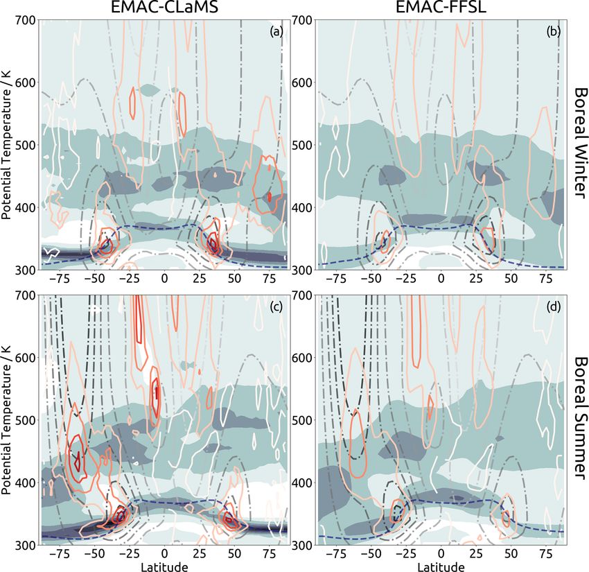
E. J. Charlesworth et al.: Lagrangian vs. Eulerian transport: investigation through age spectra 15231
3 Differences in the zonal mean state: global already found that Lagrangian transport produces higher
perspective mean age within the polar vortexes due to stronger vortex
edge transport barriers (Stenke et al., 2008; Hoppe et al.,
3.1 Mean age of air 2014). The results of this work echo those findings and
show a slightly stronger inter-representation discrepancy in
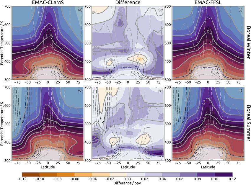
Examination of mean age of air (in Fig. 1) shows many the southern polar vortex, reaching a maximum of 0.7 years
qualitative similarities between the Lagrangian and Eule- (compared to 0.6 years in the northern polar vortex). The
rian frameworks. In both representations, mean age gradually southern polar vortex also shows stronger confinement of
increases with distance from the tropical tropopause layer the mean age differences, compared to the Northern Hemi-
(TTL), the region from 355–425 K through which most tro- sphere. In particular, the 0.4-year contour around the south-
pospheric air entering the stratosphere passes (e.g., Holton ern polar vortex extends to 75◦ S, while in the north it extends
et al., 1995; Fueglistaler et al., 2009; Butchart, 2014). At all nearly to 50◦ N. These results are likely due to the greater dy-
potential temperature levels, mean age is lowest in the trop- namical variability in the northern polar vortex (Butler et al.,
ical stratosphere (tropical pipe; Plumb, 1996) and gradually 2017). This greater dynamical variability likely causes blur-
increases towards high latitudes. Mean age is generally lower ring of the inter-representation discrepancy there, compared
in the winter than the summer, consistent with stronger win- to the more consistent southern polar vortex.
tertime downwelling in the polar region (bringing older air Above 450 K, air is mostly older in EMAC-CLaMS than
from higher to lower levels) and the isolation of the polar EMAC-FFSL. The largest differences occur at the edges
vortex (which limits the intrusion of young air from lower of the tropical pipe (around 25◦ N/S) and in the summer-
latitudes). This structure in the mean age distribution agrees time middle- and high-latitude stratosphere. The summer
well with satellite observations (Stiller et al., 2012) and other edge of the tropical pipe shows the larger differences than
models (e.g., Hauck et al., 2019). the winter edge, particularly around 600 K. This particular
The Lagrangian approach results in older air throughout point has been identified as a local minimum in diffusive ac-
most of the stratosphere. Above about 450 K, these differ- tivity by both Haynes and Shuckburgh (2000) and Abalos
ences are of a quantitative nature, and qualitatively the mean et al. (2016), suggesting that the large inter-scheme differ-
age distributions are similar during both seasons. A closer ences here (as well as the winter side of the tropical pipe)
look shows that the particular contours are in somewhat dif- are due to weaker nonphysical diffusion in EMAC-CLaMS
ferent positions, especially around the polar vortexes. In par- over EMAC-FFSL. Above 500 K in southern high latitudes,
ticular, EMAC-CLaMS results show a lower extent of old EMAC-CLaMS shows younger air than EMAC-FFSL. These
polar vortex air than EMAC-FFSL, most easily seen in the 3- differences could be caused by recirculation differences but
and 4-year contours, which are at lower altitudes in EMAC- could also be impacted by the differences in the upper bound-
CLaMS. aries of the two transport schemes (see Sect. 2.1) and will
Below 450 K there are clear qualitative differences be- therefore not be investigated further as these effects cannot
tween the representations, most visible in the 1-year contour. be readily separated.
This contour has nearly the same shape in the winter hemi- There are several other regions with notable quantitative
spheres in both transport schemes, but in the summer hemi- inter-representation differences in mean age. On the northern
sphere this contour shows a qualitative inter-representation and southern flanks of the region of horizontal outflow from
difference, particularly between 50 and 75◦ latitude. In this the tropical tropopause layer (around 35◦ N/S and 400 K)
region, between 350 and 400 K, the contour shows an eave EMAC-CLaMS shows younger air than EMAC-FFSL. This
(a vertical inversion with young air extending over the sub- difference is stronger in the winter hemisphere (greater than
tropics, resembling a roof) in EMAC-CLaMS, but in EMAC- 0.5 years) and weaker in the summer hemisphere (less than
FFSL this contour rises towards the Equator without showing 0.5 years). Although these differences are much weaker com-
an eave structure. In EMAC-CLaMS, the eave structure was pared to the differences in the polar vortexes, they are rather
found in the Northern Hemisphere during January in each large when the mean age in these regions is considered (ap-
year of the simulation; was less pronounced during October, proximately 50 % of mean age, similar to the polar vor-
November, and February; and was not found in any month texes). The differences in these regions are the counterparts
during any year in the EMAC-FFSL results. For the South- to those within the polar vortexes; in the lower stratosphere
ern Hemisphere, the eave structure was found in the EMAC- EMAC-FFSL has older air near the boundaries of the tropi-
CLaMS results in July and was less pronounced during April, cal stratosphere and younger air within the polar vortexes due
June, and August. The inter-representation mean age differ- to stronger diffusion across the latitudinal age gradient along
ences which are associated with this eave structure are ap- the polar vortex edge, creating a dipole feature in mean age
proximately half a year. differences.
Quantitative differences are largest within the polar vor-
texes, with higher mean age in EMAC-CLaMS. Other com-
parison studies of Lagrangian and Eulerian transport have
https://doi.org/10.5194/acp-20-15227-2020 Atmos. Chem. Phys., 20, 15227–15245, 2020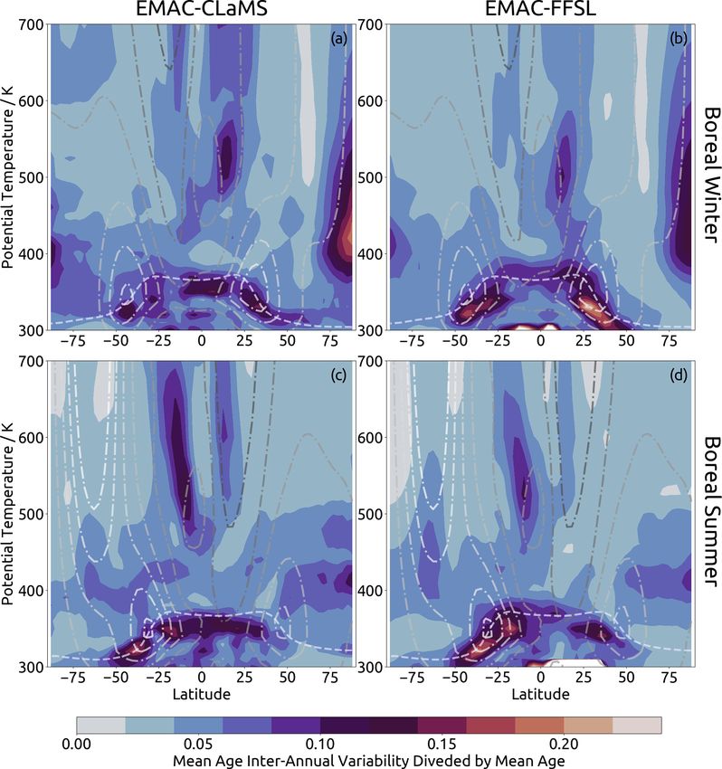
15232                      E. J. Charlesworth et al.: Lagrangian vs. Eulerian transport: investigation through age spectra

Figure 1. Mean age of air computed from age spectra for EMAC-CLaMS (a, d) and EMAC-FFSL (c, f) and the difference between them (b,
e) in boreal winter (mean of December, January, and February) (a, b, c) and boreal summer (mean of June, July, and August) (d, e, f). For
the central figures, shading shows the absolute differences (in years) between the representations (EMAC-CLaMS minus EMAC-FFSL) and
contours show percentage differences (with EMAC-FFSL as baseline). Otherwise, contours and shading show mean age (in years), with a
shading interval of 0.25 years.

3.2   Chemical composition                                             on resulting chemical composition in these regions. Quan-
                                                                       titative differences in the regions, however, depend on the
                                                                       tracer lifetime and, in the case of realistic observed chemical
Inter-representation differences in mean age are caused by
                                                                       species, the particular sources and sinks of those species.
differences in transport, meaning that simulations with chem-
                                                                          Figure 3 shows inter-representation differences in forward
ically active tracers would also show corresponding differ-
                                                                       tracer mixing ratios at various locations for exponential de-
ences in chemical composition. As an example, in Fig. 2
                                                                       cay lifetimes ranging from 1/10 of a year to 10 years. In
we consider an idealized chemical tracer with a 2-year life-
                                                                       all locations and for all lifetimes, EMAC-FFSL shows larger
time and an exponential decay globally (analogous to the
                                                                       tracer mixing ratios than EMAC-CLaMS, related to younger
E90 tracer commonly used to evaluate model transport; e.g.,
                                                                       age in these regions (compare Fig. 1). The lifetime of the
Prather et al., 2011; Abalos et al., 2017; see Sect. 2.3 for de-
                                                                       highest sensitivity to the transport scheme varies consider-
tails), which we assume to have been emitted from the trop-
                                                                       ably between the different regions. In the lowermost strato-
ical surface at a mixing ratio of 1 ppbv. Difference patterns
                                                                       sphere maximum differences occur for trace gas species with
in this 2-year lifetime tracer are largely a mirror image of
                                                                       a lifetime of a few months (red lines). In the polar vortex,
differences in mean age, as larger age means greater chem-
                                                                       on the other hand, maximum differences occur for lifetimes
ical loss for the idealized tracer from the original mixing
                                                                       of a few years (blues). Relative differences (in percent) show
ratio. However, the regions of the highest sensitivity to the
                                                                       a different dependency on lifetime (monotonic decrease), as
transport scheme differ somewhat for the 2-year tracer com-
                                                                       the tracer mixing ratio decreases with lifetime at a given lo-
pared to mean age, as the tracer is less sensitive to changes
                                                                       cation (Fig. 3). For short lifetimes, relative differences grow
in the spectrum tail. Maximum differences in tracer amount
                                                                       enormously in some regions. For instance in the polar vor-
between EMAC-FFSL and EMAC-CLaMS are found in the
                                                                       tex (both NH and SH) EMAC-FFSL tracer mixing ratios are
polar vortex (up to 40 %) and in the summertime lowermost
                                                                       higher than for EMAC-CLaMS by up to a factor of 5. The
stratosphere (up to 20 %). These results suggest that there
                                                                       southern polar vortex stands out as a region with extremely
could be substantial impacts of the chosen transport scheme

Atmos. Chem. Phys., 20, 15227–15245, 2020                                               https://doi.org/10.5194/acp-20-15227-2020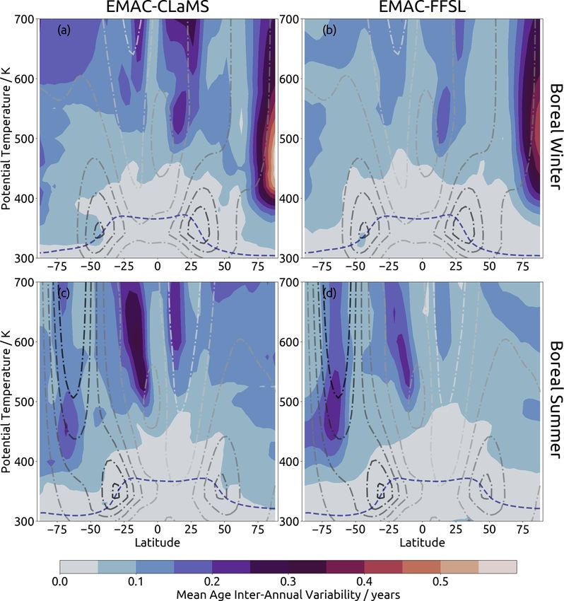
E. J. Charlesworth et al.: Lagrangian vs. Eulerian transport: investigation through age spectra                                        15233

Figure 2. Same as Fig. 1 but the quantity examined is a “forward-tracer” of 2-year lifetime (see text for details), with the exception that the
percentage differences shown in (b) and (e) use EMAC-CLaMS as the baseline (i.e., 30 % means that EMAC-FFSL results show 30 % more
forward tracer than those of EMAC-CLaMS).

large differences in the entire lifetime range below about 2              3.3   Inter-annual variability
years.
   Figure 4 presents horizontal and vertical gradients of the             Inter-annual variability in the mean age fields is shown in
2-year lifetime forward tracer. Broadly speaking, the vertical            Fig. 5. The results clearly indicate that the choice of transport
gradients are strongest along the tropopause, while the hori-             scheme affects the simulated inter-annual transport variabil-
zontal gradients are strongest at the subtropical jets, the polar         ity. In both representations the greatest variability is found
vortexes (most strongly at the southern polar vortex), and the            in the northern polar vortex and second to that at the edges
edges of the tropical pipe. While this is true in the results of          of the tropical pipe. Whereas high mean age variability is
both transport schemes, EMAC-CLaMS always shows gra-                      found in the center of the northern polar vortex, for the south-
dients which are as strong or stronger than those of EMAC-                ern polar vortex the strongest mean age variability is found
FFSL. In particular, the vertical gradients at the extratropi-            at the edge of the vortex. This is the case in both schemes
cal tropopause are approximately twice as strong in EMAC-                 and is likely to be primarily related to the frequency of sud-
CLaMS, as are the horizontal gradients at the southern po-                den stratospheric warmings, which occur much more often in
lar vortex and the edges of the tropical pipe. Meanwhile                  the northern polar vortex than the southern polar vortex. In
the horizontal gradients at the subtropical jets are approx-              EMAC-FFSL, the mean age variability at the southern polar
imately 50 % stronger in EMAC-CLaMS than in EMAC-                         vortex edge is roughly equal to the variability found at the
FFSL. These results suggest that the representation of trans-             edges of the tropical pipe. However, in EMAC-CLaMS the
port barriers is substantially stronger in EMAC-CLaMS than                variability at the edges of the tropical pipe is roughly twice as
in EMAC-FFSL. While this has been shown for the case of                   strong as the variability at the edge of the southern polar vor-
the polar vortex already by Hoppe et al. (2014), the analy-               tex. The inter-representation difference in this comparison is
sis here generalizes these findings to all the aforementioned             partially due to stronger southern polar vortex edge variabil-
stratospheric transport barriers.                                         ity in EMAC-FFSL than EMAC-CLaMS. However, this dis-
                                                                          crepancy is smaller than the inter-representation difference
                                                                          in tropical pipe edge variability; variability at the tropical
                                                                          pipe edges is about twice as strong in EMAC-CLaMS as

https://doi.org/10.5194/acp-20-15227-2020                                                 Atmos. Chem. Phys., 20, 15227–15245, 2020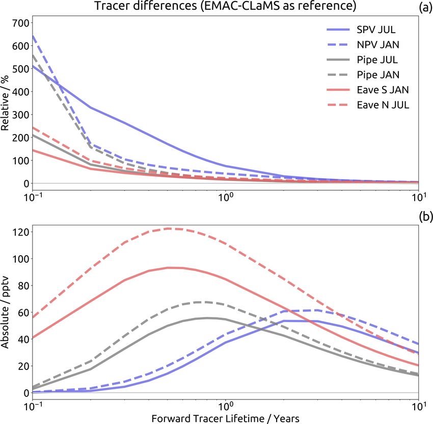
15234                      E. J. Charlesworth et al.: Lagrangian vs. Eulerian transport: investigation through age spectra

                                                                      (see Fig. 1). Analysis of the age spectra in Sect. 4.3 will shed
                                                                      more light on the reasons for the occurrence of the eaves.

                                                                      3.4   Age spectrum shape

                                                                      The age spectrum width is defined as the second moment of
                                                                      the spectra centered around the mean (e.g., Waugh and Hall,
                                                                      2002)
                                                                               Z∞
                                                                        2 1
                                                                      1 =           (τ − 0)2 G(r, t, τ ) dτ .                     (4)
                                                                          2
                                                                               0

                                                                      The width quantifies the spread or dispersion of the spectra.
                                                                         Spectrum width ranges from near zero to almost 2.5, with
                                                                      the lowest values found in the troposphere and the highest
                                                                      values found in the most troposphere-remote regions of the
                                                                      stratosphere, like the extratropical middle stratosphere and
                                                                      the polar vortexes (not shown). The summertime eave pat-
                                                                      tern in EMAC-CLaMS found in mean age and forward tracer
                                                                      contours is also seen in spectrum width as a region of higher
Figure 3. Inter-representation difference (a relative difference,
                                                                      widths (not shown).
EMAC-FFSL minus EMAC-CLaMS normalized by EMAC-                           An important parameter characterizing the shape of the
CLaMS; b: absolute difference, EMAC-FFSL minus EMAC-                  age spectra is the “ratio of moments”, which we define as
CLaMS) in forward tracer mixing ratios in several regions during      the spectrum width divided by the mean 12 / 0. The ratio of
January (“JAN”) and July (“JUL”), versus exponential decay life-      moments is also a critical parameter for estimating mean age
time of the tracer. Results are shown for the southern polar vor-     from trace gas measurements (e.g., Volk et al., 1997; Bönisch
tex (“SPV”, 70–90◦ S, 450 K), northern polar vortex (“NPV”, 70–       et al., 2009; Engel et al., 2009; Hauck et al., 2019; Hauck
90◦ S, 480 K), tropical pipe (“Pipe”, 5◦ S–5◦ N, 500 K), and sum-     et al., 2020), where the value is typically prescribed for the
mertime eave locations (“Eave”, 50◦ –75◦ north or south, 360 K).      applied inverse method.
                                                                         Figure 7 shows the ratio of moments from the age spec-
                                                                      tra. In general, the ratio of moments is relatively small in
                                                                      the tropics, related to narrow age spectra there, and increases
in EMAC-FFSL. This is also the case in the northern polar             in middle latitudes where age spectra are broader. The ra-
vortex, where mean age variability is about 50 % stronger in          tio of moments is larger in the summer compared to the
EMAC-CLaMS than in EMAC-FFSL.                                         winter hemisphere. The decrease at the upper levels and in
   Figure 6 shows inter-annual variability normalized by lo-          the polar vortex is, to some degree, related to the truncation
cal mean age. From this perspective, the northern polar vor-          of the spectra at 10 years, which causes a slight underesti-
tex still appears as a hotspot of variability and is still stronger   mate of age spectrum width. The patterns agree qualitatively
in EMAC-CLaMS than in EMAC-FFSL. Conversely, the                      with results from other models (e.g., Hall and Plumb, 1994;
southern polar vortex edge shows much weaker variability              Hauck et al., 2019). Quantitatively, the ratio values are lower
compared to other locations, due to high mean age values              than those found in the recent study by Hauck et al. (2019),
in that region, and appears to have variability of approxi-           which is related to the truncation of the spectrum tail here
mately equal magnitude in both representations. The largest           and should not be viewed as contrary to those results.
difference in this perspective from that of absolute differ-             The inter-representation ratio differences (Fig. 7b and e)
ence values is found around the tropical tropopause. Vari-            show that the ratio of moments (hence the spectrum shape)
ability in this location is stronger in EMAC-FFSL than in             is sensitive to the transport scheme used. Throughout most
EMAC-CLaMS. Furthermore, in EMAC-FFSL this variabil-                  regions of the stratosphere, the ratio of moments is larger in
ity is strongest beyond the subtropical jets, rather than at the      EMAC-FFSL than EMAC-CLaMS. The largest differences
tropical tropopause (i.e., equatorward and upward of the sub-         (up to 40 %) occur in the winter hemisphere subtropics at
tropical jets). In the case of EMAC-CLaMS, variability be-            potential temperature levels between about 350 and 450 K.
yond the subtropical jets is of a similar magnitude to vari-          In this location, EMAC-CLaMS shows very localized region
ability along the tropical tropopause. These findings could           of low spectrum moment ratios, while EMAC-FFSL shows
indicate a critical role for transport across the subtropical jets    a much weaker minima and only shows this in the southern
to cause the differences in the eave structures in the age dis-       tropics.
tribution between the Lagrangian and Eulerian frameworks

Atmos. Chem. Phys., 20, 15227–15245, 2020                                               https://doi.org/10.5194/acp-20-15227-2020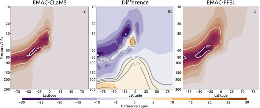
E. J. Charlesworth et al.: Lagrangian vs. Eulerian transport: investigation through age spectra                                          15235

Figure 4. Gradients of a 2-year lifetime forward tracer, from the tracer field calculated by the 10-year mean of representation age spectra.
Shown are results from EMAC-CLaMS (a, c) and EMAC-FFSL (b, d) during January (a, b) and July (c, d). The vertical gradient is calculated
with respect to potential temperature and shown in grey shading while the horizontal gradient is calculated with respect to the absolute value of
latitude and shown with the colored line contours. Plotted gradients do not have explicit units; the vertical (horizontal) gradient is normalized
to the maximum vertical (horizontal) gradient found in all four panels. Darker (redder) shading (contours) corresponds to the maximum
value, while lighter (paler) shading (contours) corresponds to the smallest values. The steps between shadings (contours) are fixed fractions
for both the filled and line contours.

   The summertime lowermost stratosphere is the only region                spheric age spectrum. This section is subdivided according
where the ratio of moments is larger in EMAC-CLaMS than                    to the regions with the most significant differences: the trop-
EMAC-FFSL. A remarkable feature is the vertical dipole in                  ical and mid-latitude stratosphere, the polar vortexes, and the
the summertime subtropical lowest stratosphere with larger                 lowermost stratosphere.
ratios below (around 350 K) smaller ratios (around 380 K).
In other words, at this location relatively broad spectra reside           4.1   Tropical and mid-latitude stratosphere
below narrower spectra. This characteristic in the ratio of mo-
ments is much more clear in EMAC-CLaMS than in EMAC-                       Air enters the stratosphere across the tropical tropopause in
FFSL and is likely related to the eave structures found in the             the TTL and is then transported upwards in the tropical pipe
mean age distribution in EMAC-CLaMS. The details of the                    by the deep branch or poleward by the shallow branch of
age spectra in this region will be investigated in Sect. 4.3.              the BDC (Brewer–Dobson circulation). Within the tropical
                                                                           pipe, with its lower edge at about 450 K, exchange with mid-
                                                                           dle latitudes is suppressed and air is thereby largely confined
4   Differences in the representation of transport                         therein (Plumb, 1996).
    processes                                                                 Figure 8b shows age spectra from EMAC-FFSL and
                                                                           EMAC-CLaMS at the 500 K level during boreal winter (Jan-
To gain further insight into inter-representation differences              uary) in the tropical pipe. Results during boreal summer
in transport processes, we turn our investigation to the strato-           are very similar (not shown). There is a clear shift of the

https://doi.org/10.5194/acp-20-15227-2020                                                  Atmos. Chem. Phys., 20, 15227–15245, 2020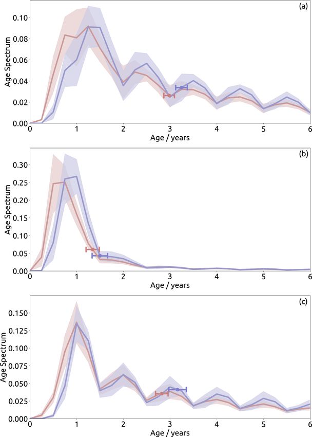
15236                    E. J. Charlesworth et al.: Lagrangian vs. Eulerian transport: investigation through age spectra

Figure 5. Standard deviation of spectra monthly-average mean age over the 10-year climatology from EMAC-CLaMS (a, c) and EMAC-
FFSL (b, d) during boreal winter (a, b) and summer (c, d).

EMAC-FFSL spectrum (red) towards younger ages for the            the same modal age (defined as the transit time at the age
transit time range below about 2 years, compared to EMAC-        spectrum peak) for EMAC-FFSL and EMAC-CLaMS. How-
CLaMS. This shift shows a higher fraction of air younger         ever, in this case EMAC-FFSL transport again clearly shows
than 9 months in EMAC-FFSL, resulting from much faster           a larger fraction of young air with transit times less than a
tropical upward transport from that transport scheme. For a      year. Similar to the case of tropical transport these differ-
transit time of 3 months (which is the age spectrum resolu-      ences must be related to stronger numerical diffusion in the
tion; see Sect. 2), EMAC-FFSL shows a substantial air mass       EMAC-FFSL transport scheme. Another interesting feature
fraction of about 4 %, whereas in EMAC-CLaMS there is no         is the stronger multiple peaks in the spectrum tail for EMAC-
such air. Results for the next transit time bin (at 6 months)    CLaMS (from ages of 3 years above). The occurrence of
are similar: the EMAC-FFSL air mass fraction is signifi-         multiple peaks in stratospheric age spectra is caused by the
cantly larger than for EMAC-CLaMS (about 0.25 compared           seasonality of transport into the stratosphere (Reithmeier and
to 0.075). As 3 months is beyond the fastest transit time from   Sausen, 2008; Ploeger and Birner, 2016). Stronger numerical
the middle troposphere to 500 K based on large-scale up-         diffusion in EMAC-FFSL blurs this seasonal transport signal
welling velocities (Wright and Fueglistaler, 2013), the dif-     over the course of a few years.
ferences at short transit times can only be caused by stronger      Very similar conclusions hold for the Southern Hemi-
vertical diffusion due to numerical diffusion in the FFSL        sphere middle latitudes during austral winter (Fig. 8a). The
transport scheme.                                                fraction of young air (age below about 1 year) here is greater
   Comparison of age spectra in northern middle latitudes at     in EMAC-FFSL compared to EMAC-CLaMS, related to
the same level (Fig. 8c) shows smaller differences and even

Atmos. Chem. Phys., 20, 15227–15245, 2020                                        https://doi.org/10.5194/acp-20-15227-2020
E. J. Charlesworth et al.: Lagrangian vs. Eulerian transport: investigation through age spectra                                    15237

Figure 6. Same as Fig. 5, but the quantity shown is the standard deviation of spectrum mean age scaled (divided) by the spectrum mean age.

stronger diffusion of the transport scheme, and the peaks in           sive transport across the vortex edge in the FFSL transport
the spectrum tail are again weaker.                                    scheme. This difference suggests that simulations of chemi-
                                                                       cally active tracers with short stratospheric lifetimes and tro-
4.2   Polar vortex                                                     pospheric origins would show substantially stronger south-
                                                                       ern polar vortex concentrations in EMAC-FFSL, compared
Due to strong polar downwelling motion and the cyclonic                to EMAC-CLaMS. For long-lived trace gas species differ-
circumpolar flow, air masses inside the wintertime strato-             ences would be smaller. Consequently, the amount of ozone-
spheric polar vortexes are largely isolated against exchange           depleting substances in polar regions with lifetimes below a
with middle latitudes, even more so in the Southern Hemi-              few years and related polar ozone loss can substantially differ
sphere, where the cyclonic circumpolar flow is stronger than           depending on the chosen transport scheme.
in the Northern Hemisphere. Figure 9b shows the age spectra               Variability in the age spectra seems to be roughly similar
within the southern stratospheric polar vortex. Below 3 years,         at most ages but is substantially different below 3 years of
the spectra show clear qualitative differences. EMAC-FFSL              age, with much more variability in EMAC-CLaMS at the 2.5-
shows two peaks in this region: one at 2.5 years and the other         year peak and much more variability in EMAC-FFSL below
at 1.25 years. Meanwhile EMAC-CLaMS shows only one                     2 years of age. At ages older than 3 years, the age spectra
peak, which is at 2.5 years. The common peak at 2.5 years              are qualitatively similar, showing multiple maxima at 1-year
is much stronger in EMAC-CLaMS than in EMAC-FFSL.                      intervals at the half-year marks and regular minima at the 1-
The contribution from air younger than 2 years is about twice          year marks. This means stronger contribution of air emitted
as strong in EMAC-FFSL as in EMAC-CLaMS. This much                     during January and weaker contribution of air emitted during
higher fraction of young air inside the polar vortex in EMAC-          July. Both schemes show this quality, with EMAC-CLaMS
FFSL than in EMAC-CLaMS is caused by stronger diffu-

https://doi.org/10.5194/acp-20-15227-2020                                             Atmos. Chem. Phys., 20, 15227–15245, 2020
15238 E. J. Charlesworth et al.: Lagrangian vs. Eulerian transport: investigation through age spectra
Figure 7. Panels correspond to those of Fig. 2, but the quantity shown is the age spectra ratio of moments (width divided by mean age, units
of years).
showing a greater difference between the contributions at the these two regions have a similar age. As the mean age and
maxima and minima. forward tracer contours in Figs. 1 and 2 in the upper region
Figure 9a shows age spectra within the northern polar vor- follow similar paths in both representations, transport from
tex. As in the southern polar vortex, ages above 3 years show the upper region into the lower region is not likely to play a
qualitative similarity between the representations; maxima in role in the discrepancy of the eave structure representation.
the spectra correspond to January-emitted tracers while min- Therefore, the eave structure, as present in EMAC-CLaMS,
ima correspond to July-emitted tracers. At ages younger than probably arises from weaker direct transport from the tropo-
2.75 years, EMAC-FFSL shows greater tracer concentrations sphere (i.e., not through the tropical tropopause layer) into
than EMAC-CLaMS. However, the difference between the the lower eave region, in comparison to EMAC-FFSL.
two representations in this location for young ages is much To gain more insight into the underlying processes, Fig. 10
smaller than the difference in the southern polar vortex, while shows the corresponding age spectra for the two schemes at
variability in the age spectra is much stronger (approximately the 360 and 400 K levels between 50–60◦ latitude. In both
a factor of 2) in EMAC-CLaMS than in EMAC-FFSL. cases, the upper-level age spectra are very similar in both
EMAC-FFSL and EMAC-CLaMS. In the Southern Hemi-
4.3 Lowermost stratosphere sphere in particular, these spectra are nearly identical, with
only slightly more tracer between 0.5 and 1.5 years of age
A particularly interesting feature in the mean age and tracer found in EMAC-CLaMS. Meanwhile the Northern Hemi-
distributions in the summertime lowermost stratosphere in sphere results show somewhat less agreement between the
Figs. 1 and 2 is the eave structure. The structure – only found two representations in the upper levels, with slightly less
in EMAC-CLaMS – has two features: an old-air region at the tracer at 0.25 years and somewhat more tracer between 0.5
level of the subtropical jet (around 360 K) and a young-air re- and 1.0 years in EMAC-CLaMS. However, there is consid-
gion above that (around 400 K). Conversely, in EMAC-FFSL
Atmos. Chem. Phys., 20, 15227–15245, 2020 https://doi.org/10.5194/acp-20-15227-2020E. J. Charlesworth et al.: Lagrangian vs. Eulerian transport: investigation through age spectra 15239
Figure 9. Age spectra from EMAC-FFSL (red) and EMAC-CLaMS
(blue) within (a) the northern polar vortex (480 K, 70–90◦ N, Jan-
uary) and (b) the southern polar vortex (90–70◦ S 450 K, July).
Lines indicate multi-annual mean with shading showing annual
variability. Dots indicate mean age of spectra, with surrounding bars
showing annual variability. Variability for both quantities is com-
puted as 2 standard deviations.
Figure 8. Age spectra from the results of EMAC-FFSL (red) and transported into the region by the shallow branch of the BDC
EMAC-CLaMS (blue) at 500 K for (a) the southern mid-latitude (e.g., Bönisch et al., 2009). In spring and summer, a new
stratosphere (40–60◦ S, July), (b) the tropical pipe (6◦ S–6◦ N, Jan- transport pathway emerges which is related to upward trans-
uary), and (c) the northern mid-latitude stratosphere (40–60◦ N, port in the tropics and poleward transport directly above the
January). Lines indicate multi-annual mean, with shading showing subtropical jet, and it is characterized by transport timescales
annual variability. Dots indicate mean age of spectra, with surround- of about half a year to 1.5 years. This poleward transport hap-
ing bars showing annual variability. Variability for both quantities pens in the layer of about 380–450 K, which belongs to the
is computed as 2 standard deviations.
region above the subtropical jet and below the tropical pipe.
Fast transport in this layer agrees well with the existence of a
tropically controlled transition region for water vapor as pro-
erable inter-representation difference in the relationship be- posed by Rosenlof et al. (1997). The EMAC-CLaMS simula-
tween the age spectra in the upper region and the lower tion shows a clear age inversion related to this flushing of the
region; EMAC-FFSL results show nearly identical spectra extratropical lowermost stratosphere with young air above
in both regions, while EMAC-CLaMS shows a consistent the jet. In the EMAC-FFSL simulation, on the other hand,
difference in the upper and lower region spectra. In the this feature is totally absent because a much higher fraction
EMAC-CLaMS spectra for both hemispheres, the upper re- of young air with transit times shorter than 0.5 years blurs
gion shows more air younger than 0.5 years while the lower the old-air signature in the layer around 350 K.
region shows more air between 0.5 years and 1.5 years, and Hence, the Lagrangian and Eulerian transport schemes
both regions show nearly identical contributions from air at result in different preferences for transport pathways into
0.5 years. the summertime lowermost stratosphere: poleward transport
The differences in age spectra, mean age, and tracer mix- above the jet (Lagrangian) versus cross-tropopause trans-
ing ratios suggest that the eave structure in the lowermost port at levels below (Eulerian). It remains to be shown from
stratosphere is caused by an interplay of transport processes trace gas observations in the lowermost stratosphere whether
as described in the following. The lowermost stratosphere the eave structure evident in the age distribution from La-
mean age distribution results from a mixture of old air masses grangian transport is a feature of the observed atmosphere.
downwelling from the stratosphere and young air masses Initial indications for a mixture of old wintertime air and
https://doi.org/10.5194/acp-20-15227-2020 Atmos. Chem. Phys., 20, 15227–15245, 202015240 E. J. Charlesworth et al.: Lagrangian vs. Eulerian transport: investigation through age spectra
than the model generation before (Forster et al., 2020), fur-
ther fueling discussion about solar geoengineering.
A modeling effort to assess the opportunities and risks
of solar geoengineering using stratospheric sulfate aerosols
within the Geoengineering Large Ensemble (GLENS)
project has recently been presented by Tilmes et al. (2018). In
this project, injection strategies have been proposed to main-
tain the distribution of global surface temperatures in the
future, and potential side effects (e.g., on precipitation and
stratospheric ozone) have been discussed (Kravitz and Dou-
glas, 2020). Although the results of that work suggest that
it may be possible to use SAI successfully (i.e., to maintain
the global distribution of surface temperatures), the authors
note that a main uncertainty in their model results is related
to stratospheric transport processes and their representation
in current climate models.
Our model experiment, which applies one climate model
with two different transport schemes in the same simula-
tion, is well-suited to shed further light on this uncertainty
of geoengineering projections related to uncertainties in air
mass dispersal due to the model representation of strato-
Figure 10. Age spectra from the results of EMAC-FFSL (red) and spheric transport. It is noteworthy here that this discussion
EMAC-CLaMS (blue) within the summertime lowermost strato-
concerns air mass transport and not the transport of sulfate,
sphere regions of the eave structures at 360 K (sold lines) and 400 K
as our simulation does not include stratospheric chemistry.
(dashed lines) in (a) the Northern Hemisphere (55–75◦ N, July) and
(b) the Southern Hemisphere (55–75◦ S, January). However, we consider a state-of-the-art transport scheme
(EMAC-FFSL) which is also applied in other current climate
models and a novel Lagrangian scheme (EMAC-CLaMS)
which has significantly less numerical diffusion. As results
young air masses from transport above the subtropical jet
from this paper show, two regions emerge where transport
in that region during early spring have already been found
differences between the two representations are especially
in aircraft in situ measurements of N2 O and CO by Krause
large: the lowermost stratosphere and the polar vortex. Both
et al. (2018).
are critical regions for the processes which affect the efficacy
of SAI. In particular, sulfate concentrations in the lowermost
stratosphere crucially affect radiative forcing, whereas sul-
5 Discussion fate concentrations in the polar vortex control the side effects
of geoengineering on stratospheric ozone.
The results of the work presented thus far have shown sub- To illustrate the potential differences in geoengineering
stantial differences in tracer transport between EMAC-FFSL simulations caused by model transport representation, we
and EMAC-CLaMS. Given that the FFSL transport scheme modified our experiments to include continuous point-source
used by EMAC is also used in a wide array of other cli- injections of tracers with idealized chemistry. The injection
mate models, the effects of unphysical numerical diffusion is handled by forcing the tracer mixing ratio to 1 ppbv within
in EMAC-FFSL which have been described here are likely a region of nine EMAC grid cells (three cells wide both
to affect tracer transport in other climate models as well. east–west and north–south). The idealized chemistry is rep-
This could cause complications for the interpretation of re- resented by a global exponential decrease with 30, 90, and
sults from these models, especially for stratospheric trans- 365 d lifetimes. Figure 11 shows the dispersal of a 365 d life-
port. One such topic, for which there is considerable model- time tracer which was injected at 30◦ N and 180◦ E at the
ing activity at the moment, is geoengineering through strato- 89 hPa pressure level. The results are shown for the two trans-
spheric aerosol injection (SAI). This has been proposed as port schemes after about 5 years of simulation and the re-
a method to reduce or entirely offset the surface temper- sults represent the state of the simulation on a single time
ature effects of global warming (e.g., Crutzen, 2006) and step. Both models show three regions with high tracer mix-
is likely to gather more attention as the global mixing ra- ing ratios: (1) a plume between 300 and 330◦ E which is the
tios of greenhouse gases rise. Relatedly, the latest-generation most prominent feature of the snapshot, (2) a second plume
climate models from the Coupled Model Intercomparison west of 260E and between 40–50◦ S, (3) and then a third lo-
Project Phase 6 (CMIP6) show an even stronger equilibrium cal maxima of tracer mixing ratios in the upper northwest
climate sensitivity and simulate stronger climate warming corner of the image. In the EMAC-FFSL results, this lat-
Atmos. Chem. Phys., 20, 15227–15245, 2020 https://doi.org/10.5194/acp-20-15227-2020You can also read