Is it Enough to Optimize CNN Architectures on ImageNet?
←
→
Page content transcription
If your browser does not render page correctly, please read the page content below
Is it Enough to Optimize CNN Architectures on
                                                                     ImageNet?

                                                             Lukas Tuggener1,2 , Jürgen Schmidhuber2,3 , Thilo Stadelmann1,4
                                            1
                                                ZHAW Centre for Artificial Intelligence, Winterthur, Switzerland, 2 University of Lugano, Switzerland
                                                                             3
                                                                               The Swiss AI Lab IDSIA, Switzerland
                                                             4
                                                               Fellow of the European Centre for Living Technology, Venice, Italy
arXiv:2103.09108v2 [cs.CV] 9 Jun 2021

                                                                        {tugg,stdm}@zhaw.ch, juergen@idsia.ch

                                                                                         Abstract
                                                      An implicit but pervasive hypothesis of modern computer vision research is that
                                                      convolutional neural network (CNN) architectures which perform better on Im-
                                                      ageNet will also perform better on other vision datasets. We challenge this hy-
                                                      pothesis through an extensive empirical study for which we train 500 sampled
                                                      CNN architectures on ImageNet as well as 8 other image classification datasets
                                                      from a wide array of application domains. The relationship between architecture
                                                      and performance varies wildly, between the datasets. For some of the datasets the
                                                      performance correlation with ImageNet is even negative. Clearly, it is not enough
                                                      to optimize architectures solely for ImageNet when aiming for progress that is
                                                      relevant for all applications. We identify two dataset-specific performance indica-
                                                      tors: the cumulative width across layers as well as the total depth of the network.
                                                      Lastly, we show that the range of dataset variability covered by ImageNet can be
                                                      significantly extended by adding ImageNet subsets restricted to fewer classes.

                                        1        Introduction
                                        Deep convolutional neural networks (CNNs) are the core building block for most modern visual
                                        recognition systems. In the past several years they have lead to major breakthroughs in many
                                        domains of computer perception. Since the inception of the field the community has been searching
                                        the high dimensional space of possible network architectures for models with desirable properties.
                                        Important milestones such as DanNet [1], AlexNet [2], VGG [3], HighwayNet [4], and ResNet [5] (a
                                        HighwayNet with open gates) can be seen as update steps in this stochastic optimization problem and
                                        stand testament that this manual architecture search works. But it is of great importance that the right
                                        metrics are used during the search for new neural network architectures. Only when we measure
                                        performance with a truly meaningful metric is it certain that a new high-scoring architecture is also
                                        fundamentally better.
                                        It would be desirable to construct such a metric form a solid theoretical understanding of deep CNNs.
                                        Due to the absence of a solid theoretical basis novel neural network designs are tested in an empirical
                                        fashion. Traditionally model performance has been judged using accuracy point estimates [2, 6, 3].
                                        This simple measure ignores important aspects such as model complexity and speed. Newer work
                                        addresses this issue by reporting a curve of the accuracy at different complexity settings of the model,
                                        highlighting how well a design deals with the accuracy versus complexity tradeoff [7, 8].
                                        Very recent work strives to improve the quality of the empiric evaluation even further. There have
                                        been attempts to use extensive empirical studies to discover general rules on neural network design
                                        [9, 10, 11, 12], instead of simply showing the merits of a single neural network architecture. Another
                                        line of research aims to improve empiricism by sampling whole populations of models and comparing
                                        error distributions instead of individual scalar errors [13].

                                        Preprint. Under review.
We acknowledge the importance of the above-                                             1.0
mentioned improvements in the empirical meth-

                                                        Relative target dataset error
ods used to test neural networks, but identify a                                        0.8
weak spot that runs trough the above-mentioned
work: the heavy reliance on ImageNet [14] (and                                          0.6
to some extent the very similar Cifar100 [15]).
In 2011, Torralba and Efros already pointed out                                         0.4
that visual recognition datasets that were built
to represent the visual world tend to become                                            0.2
a small world in themselves [16]. Objects are
no longer in the dataset because they are impor-                                        0.0
tant, they are important because they are in the                                              30   40    50     60    70   80
                                                                                                       ImageNet error
dataset. A large part of computer vision research                                             ImageNet      Powerline      Insects
has lived in the ImageNet world for almost a
decade now, and consequently worked under the
implicit assumption that ImageNet is large and      Figure 1: Is a CNN architecture that performs well
diverse enough to represent the visual world. In    on ImageNet necessarily a good choice for a dif-
this paper we challenge this assumption and ask     ferent vision dataset? This plot suggests otherwise:
the question: Do neural network architecture        It displays the relative test errors of 500 randomly
improvements achieved on ImageNet generalize        sampled CNN architectures on three datasets (Ima-
to other datasets?                                  geNet, Powerline, and Insects) plotted against the
                                                    test error of the same architectures on ImageNet.
We answer this question with an extensive empir-    The architectures have been trained from scratch
ical investigation. As a tool for this investigationon all three datasets. Architectures with low er-
we introduce the notion of architecture and per-    rors on ImageNet also perform well on Insects, on
formance relationship (APR). The performance        Powerline the opposite the case.
of a CNN architecture does not exist in a vac-
uum, it is only defined in relation to the dataset
on which it is used. This dependency is what we call APR induced by a dataset. We study the
change in APRs between datasets by sampling 500 neural network architectures and training all
of them on a set of datasets1 . We then compare errors of the same architectures across datasets,
revealing the changes in APR (see Figure 1). This approach allows us to study the APRs induced
by different datasets on a whole population of diverse network designs rather than just a family of
similar architectures such as the ResNets [5] or MobileNets [17].
All of our code, data and trained models will be made publicly available to ensure reproducibility and
facilitate future research.

2   Related Work

Neural network design. With the introduction of the first deep CNNs [1, 2] the design of neural
networks immediately became an active research area. In the following years many improved
architectures where introduced, such as VGG [3], Inception [18], HighwayNet [4], ResNet [5]
(a HighwayNet with open gates), ResNeXt [7], or MobileNet [17]. These architectures are the
result of manual search aimed at finding new design principles that improve performance, for
example increased network depth and skip connections. More recently, reinforcement learning [8],
evolutionary algorithms [19] or gradient descent [20] have been successfully used to find suitable
network architectures automatically. Our work relates to manual and automatic architecture design
because it adds perspective on how widely certain improvements are applicable.
Empirical studies. In the absence of a solid theoretical understanding, large-scale empirical studies
are the best tool at our disposal to gain insight into the nature of deep neural networks. These studies
can aid network design [21, 22, 23] or be employed to show the merits of different approaches, for
example that the classic LSTM [24] architecture can outperform more modern models [25], when
it is properly regularised. More recently, empirical studies have been used to infer more general

   1
     Since we only sample models in the complexity regime of 340 mega flops (MF) to 400MF (ResNet-152
has 11.5GF) we could complete the necessary 7500 model trainings within a moderate 85 GPU days on Tesla
V100-SXM2-32GB GPUs.

                                                    2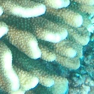
Table 1: Meta data of the used datasets.

           DATASET         N O . I MAGES   N O . C LASSES    I MG . S IZE        D OMAIN
           C ONCRETE           40K                2          227 × 227        M AINTENANCE
           MLC2008             43K                9          312 × 312          B IOLOGY
           I MAGENET           1.3M             1000         256 × 256      E VERYDAY OBJECTS
           HAM10000            10K                7          296 × 296           M EDICAL
           P OWERLINE           8K                2          128 × 128         M AINTENANCE
           I NSECTS            63K               291         296 × 296           B IOLOGY
           NATURAL              25K               6          150 × 150       NATURAL S CENES
           C IFAR 10            60K              10           32 × 32       E VERYDAY OBJECTS
           C IFAR 100           60K              100          32 × 32       E VERYDAY OBJECTS

rules on the behaviour of neural networks such as a power-law describing the relationship between
generalization error and dataset size [9] or scaling laws for neural language models [11].
Generalization in neural networks. Despite their vast size have deep neural networks shown
in practice that they can generalize extraordinarily well to unseen data stemming from the same
distribution as the training data. Why neural networks generalize so well is still an open and very
active research area [26, 27, 28]. This work is not concerned with the generalization of a trained
network to new data, but with the generalization of the architecture design progress itself. Does an
architecture designed for a certain dataset, e.g. natural photo classification using ImageNet, work
just as well for medical imaging? There has been work investigating the generalization to a newly
collected test set, but in this case the test set was designed to be of the same distribution as the original
training data [29].
Neural network transferability It is known that the best architecture for ImageNet is not necessarily
the best base architecture for other applications such as semantic segmentation [30] or object detection
[31]. Researchers who computed a taxonomy of multiple visions tasks identified that the simmilarities
between tasks did not depend on the used architecture [32]. Research that investigates the relation
between model performance on ImageNet and new classification datasets in the context of transfer
learning [33, 34] suggests that there is a strong correlation which is also heavily dependent on the
training regime used [35]. Our work differs form the ones mentioned above in that we are not
interested in the transfer of learned features but transfer of the architecture designs and therefore we
train our networks from scratch on each dataset. Moreover do we not only test transferability on a
few select architectures but on a whole network space.
Neural network design space analysis. Radosavovic et al. [13] introduced network design spaces
for visual recognition. They define a design space as a set of architectures defined in a parametric
form with a fixed base structure and architectural hyperparameters that can be varied, similar to the
search space definition in neural architecture search [8, 19, 20]. The error distribution of a given
design space can be computed by randomly sampling model instances from it and computing their
training error. We use a similar methodology but instead of comparing different design spaces, we
compare the results of the same design space on different datasets.

3   Datasets
To enable cross dataset comparison of APRs we assembled a corpus of datasets. We chose datasets
according to the following principles: (a) include datasets from a wide spectrum of application areas,
such that generalization is tested on a diverse set of datasets; (b) only use datasets that are publicly
available to anyone to ensure easy reproducibility of our work. Table 1 shows some meta-data of the
chosen datasets. For more detailed dataset descriptions and example images please see chapter A and
Figure 9 in the appendix.

                                                       3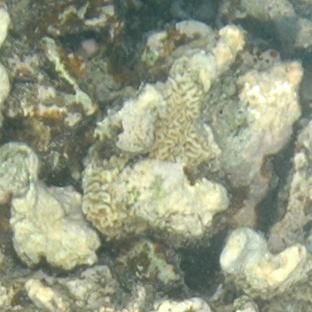
Table 2: Dataset-specific experimental settings.

                       DATASET        NO.   TRAINING EPOCHS               E VAL .   ERROR

                       CONCRETE                 20                             TOP -1
                       MLC2008                  20                             TOP -1
                       I MAGENET                10                             TOP -5
                       HAM10000                 30                             TOP -1
                       P OWERLINE               20                             TOP -1
                       I NSECTS                 20                             TOP -5
                       NATURAL                  20                             TOP -1
                       C IFAR 10                30                             TOP -1
                       C IFAR 100               30                             TOP -5

4     Experiments and Results

4.1   Experimental setup

We sample our architectures form the very gen-
eral AnyNetX [36] parametric network space.
                                                                                         mxnx3
The networks in AnyNetX consist of a stem, a         Stem
body, and a head. The body performs the ma-                              Conv2D - kernel: 3x3, stride: 2, out: 32
jority of the computation, stem and head are
kept fixed across all sampled models. The body                                           m/2 x n/2 x 32
consists of four stages, each stage i starts with
a 1 × 1 convolution with stride si , the remain-            Stage 1 (d1,w1,b1,g1,s1=1)

der is a sequence of di identical blocks. The                 Conv2D - kernel: 1x1, stride: s1, out:w1

blocks are standard residual bottleneck blocks                 Block 1

with group convolution [7], with a total block
width wi , bottleneck ratio bi and a group width                 Conv2D - k: 1x1, out: w1 /b1

gi (into how many parallel convolutions the total                Conv2D - k: 3x3, out: w1 /b1, groups:g1
width is grouped into). Within a stage, all the                  Conv2D - k: 1x1, out: w1         Conv2D - k: 1x1, out: w1
block parameters are shared. See Figure 2 for a
comprehensive schematic.
                                                     Body

The AnyNetX design space has a total of 16                     Block 2
degrees of freedom, having 4 stages with 4 pa-                                              ...
rameters each. We obtain our model instances                   Block d1
by performing log-uniform sampling of di ≤ 16,
wi ≤ 1024 and divisible by 8, bi ∈ 1, 2, 4, and                                          m/2 x n/2 x w1

gi ∈ 1, 2, ..., 32. The stride si is fixed with a           Stage 2 (d2,w2,b2,g2,s2=2)

stride of 1 for the first stage and a stride of 2                                        m/4 x n/4 x w2
for the rest. We repeatedly draw samples until              Stage 3 (d3,w3,b3,g3,s3=2)
we have obtained a total of 500 architectures in
                                                                                         m/8 x n/8 x w3
our target complexity regime of 360 mega flops
(MF) to 400 MF. We use a very basic training                Stage 4 (d4,w4,b4,g4,s4=2)

regime that consists of only flipping and crop-
                                                                                         m/16 x n/16 x w4
ping of the inputs in conjunction with SGD plus
momentum and weight decay. The same 500
                                                     Head

                                                                          FullyConnected - size: c
models are trained on each dataset until the loss
is reasonably saturated. The exact number of                                             1x1xc

epochs has been determined in preliminary ex-
periments and depends on the dataset (see Table     Figure 2: The structure of models in the AnyNetX
2). For extensive ablation studies ensuring the     design space, with a fixed stem and a head, consist-
empirical stability of our experiments with re-     ing of one fully-connected layer of size c, (where c
spect to Cifar10 performance, training duration,    is the number of classes). Each stage i of the body
training variability, top-1 to top-5 error com-     is parametrised by di , wi , bi , gi , the strides of the
parisons, overfitting and class distribution see    stages are fixed with s1 = 1 and si = 2 for the
chapters B.1 to B.7 in the appendix.                remainder.

                                                    4
4.2   Experimental results

As a preliminary analysis we compute the em-
pirical cumulative error distribution function
                                                                                                                                    1.0

                                                                                      eCDF(x): share of models with error below x
(eCDF ) per dataset. The eCDF of n models
with errors ei is defined as:
                                                                                                                                    0.8
                                    n
                    1X
         eCDF (e) =       1[ei < e],                             (1)
                    n i=1                                                                                                           0.6
                                                                                                                                                                                   Concrete
                                                                                                                                                                                   MLC 2008
meaning eCDF (x) returns the fraction of mod-          0.4                                                                                                                         ImageNet
els with an error smaller than x. Figure 3                                                                                                                                         HAM10000
                                                                                                                                                                                   Powerline
shows the eCDF per dataset. ImageNet ex-               0.2                                                                                                                         Natural
hibits a steady decrease in model performance                                                                                                                                      Insects
and very large spread between the best and the                                                                                                                                     Cifar10
                                                       0.0                                                                                                                         Cifar100
worst architectures. Natural, Insects, Power-
line and Cifar100 have a somewhat similarly                0                                                                                             20         40          60        80
                                                                                                                                                            test error on dataset
shaped eCDF , with a relatively high density
of good architectures and a long tail contain- Figure 3: eCDF plots from the 500 sampled archi-
ing significantly worse architectures. Concrete, tectures for each dataset. The y coordinate gives
HAM10000, MLC2008 and Cifar10 show a dif- the share of models with less error than the corre-
ferent picture. The eCDF s of these datasets sponding x value.
are narrow, indicating a low difference in perfor-
mance for most of the sampled architectures. The error percentage for Concrete is below 0.5 percent
for almost all of the sampled architectures, indicating that this dataset is easy to learn for modern
CNN architectures.
                 Insects - :0.967               MLC 2008 - corr:0.499                                                                HAM10000 - :0.517               Cifar100 - :0.476
          40                             35.0                                    30
                                         32.5
                                                                                                                                                              50
          30                                                                     28
                                         30.0                                    26                                                                           40
          20
                                         27.5                                                                                                                 30
          10                                                                     24
                                         25.0
                                                                                 22                                                                           20
          0                              22.5
                40        60       80            40        60           80                                                           40         60       80          40         60        80
                 Concrete - :0.001               Cifar10 - :-0.104                                                                   Powerline - :-0.436               Natural - :-0.38
                                                                                 50                                                                           80
          1.5
                                         40                                      40
                                                                                                                                                              60
          1.0                                                                    30
                                         30                                                                                                                   40
                                                                                 20
          0.5
                                                                                 10
                                         20                                                                                                                   20
          0.0                                                                     0
                40         60       80          40         60           80                                                            40       60        80          40         60        80

Figure 4: Test errors of all 500 sampled architectures on target datasets (y-axis) plotted against the test
errors of the same architectures (trained and tested) on ImageNet (x-axis). The top 10 performances
on the target datasets are plotted in orange and the worst 10 performances in red.

We analyze the architecture-performance relationship (APRs) in two ways. For every target dataset
(datsets which are not ImageNet) we plot the test error of every sampled architecture against the test
error of the same architecture (trained and tested) on ImageNet, visualizing the relationship of the
target dataset’s APR with the APR on ImageNet. Second, we compute Spearman’s ρ rank correlation
coefficient [37]. It is a nonparametric measure for the strength of the relation between two variables
(here the error on the target datasets with the error of the same architecture on ImageNet). Spearman’s
ρ is defined on [−1, 1], where 0 indicates no relationship and −1 or 1 indicates that the relationship
between the two variables can be fully described using only a monotonic function.
Figure 4 contains the described scatterplots with the corresponding correlation coefficients in the
title. The datasets plotted in the top row show a strong (Insects) or medium (MLC2008, HAM10000,
Cifar100) error correlation with ImageNet. This confirms that many classification tasks have an
APR similar to the one induced by ImageNet, which makes ImageNet performance a decent archi-
tecture selection indicator for these datasets. The errors on Concrete are independent of the their
corresponding ImageNet counterparts since the accuracies are almost saturated with errors between
0 and 0.5. This has implications for practical settings, where in such cases suitable architectures

                                                                             5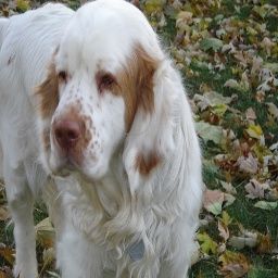
ImageNet - :-0.205                                                 Insects - :-0.2                                                HAM10000 - :0.296

                   Cumulated - Block Depth

                                                                                                                                                    Cumulated - Block Depth
                                             40                                                                                                                               40

                                                                                 Cumulated - Block Depth
                                                                                                           40
                                             30                                                            30                                                                 30
                                             20                                                            20                                                                 20
                                             10                                                            10                                                                 10
                                                        40        60        80                                  0        10        20    30    40                                  22      24   26    28        30
                                                      Powerline - :0.742                                                 Natural - :0.527                                               Cifar100 - :0.527

                   Cumulated - Block Depth

                                                                                 Cumulated - Block Depth

                                                                                                                                                    Cumulated - Block Depth
                                             40                                                            40                                                                 40
                                             30                                                            30                                                                 30
                                             20                                                            20                                                                 20
                                             10                                                            10                                                                 10
                                                  0          20        40                                           20        40        60    80                                   20      30    40        50

Figure 5: Errors of all 500 sampled architectures on ImageNet, Insects, HAM10000, Powerline,
Natural, and Cifar100 (x-axis) plotted against the cumulative block depths (y-axis).

should be chosen according to computational considerations rather than ImageNet performance, and
reinforces the idea that practical problems may lie well outside of the ImageNet visual world [38].
The most important insight from Figure 4, however, is that some datasets have a slight (Cifar10) or
even strong (Powerline, Natural) negative error correlation with ImageNet. Architectures which
perform well on ImageNet tend perform sub-par on these datasets. A visual inspection shows that
some of the very best architectures on ImageNet perform extraordinarily poor on these three datasets.
With this evidence we can safely reject the hypothesis that increasing performance on ImageNet
implies increased performance on other image classification tasks.

4.3   Identifying Drivers of Difference between Datasets

The block width and depth parameters of the top 15 architectures for ImageNet (see Figure 21 in the
appendix) follow a clear structure: they consistently start with low values for both block depth and
width in the first stage, then the values steadily increase across the stages for both parameters. The
error relationships observed in Figure 4 are consistent with how well these patterns are replicated
by the other datasets. Insects shows a very similar pattern, MLC2008 and HAM10000 have the
same trends but more noise. Powerline and Natural clearly break from this structure, having a flat or
decreasing structure in the block with and showing a quite clear preference for a small block depth in
the final stage. Cifar10 and Cifar100 are interesting cases, they have the same behaviour as ImageNet
with respect to block width but a very different one when it comes to block depth.
We thus investigate the effect of the cumulative block depth (summation of the depth parameter
for all four stages, yielding the total depth of the architecture) across the whole population of
architectures by plotting the cumulative block depth against the test error for the six above-mentioned
datasets. Additionally, we compute the corresponding correlation coefficients. Figure 5 shows that
the best models for ImageNet have a cumulative depth of at least 10. Otherwise there is no apparent
dependency between the ImageNet errors and cumulative block depth. The errors of Insects do not
seem to be related to the cumulative block depth at all. HAM10000 has a slight right-leaning spread
leading to a moderate correlation, but the visual inspection shows no strong pattern. The errors on
Powerline, Natural, and Cifar100 on the other hand have a strong dependency with the cumulative
block depth. The error increases with network depth for all three datasets. with the best models all
having a cumulative depth smaller than 10.
We also plot the cumulative block widths against the errors and compute the corresponding correlation
coefficients for the same six datasets (see Figure 6). We observe that the ImageNet errors are
negatively correlated with the cumulative block width, and visual inspection shows that a cumulative
block width of at least 250 is required to achieve a decent performance. The errors on Insects and
HAM10000 replicate this pattern to a lesser extent, analogous to the top 15 architectures. Powerline
and Natural have no significant error dependency with the cumulative block width, but Cifar100 has
an extremely strong negative error dependency with the cumulative block width, showing that it is
possible for a dataset to replicate the behaviour on ImageNet in one parameter but not the other. In
the case of Cifar100 and ImageNet, low similarity in block depth and high similarity in block width
yield a medium overall similarity of ARPs on Cifar100 and Imagenet. This is consistent with the
overall relationship of the two datasets displayed in Figure 4.

                                                                                                                              6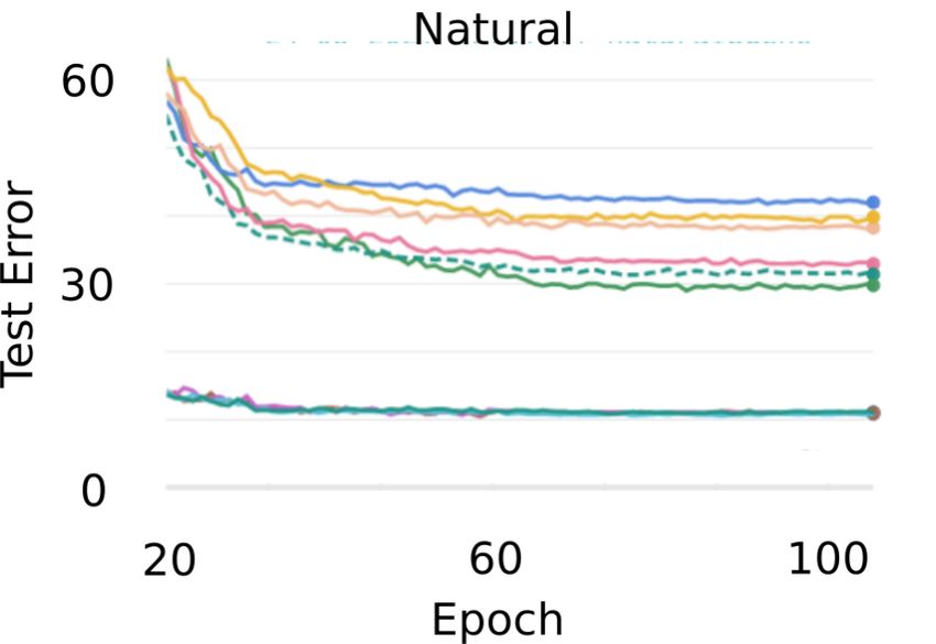
ImageNet - :-0.511 Insects - :-0.459 HAM10000 - :-0.354
1250 1250 1250
Cumulated - Block Width
Cumulated - Block Width
Cumulated - Block Width
1000 1000 1000
750 750 750
500 500 500
250 250 250
0 0 0
40 60 80 0 10 20 30 40 22 24 26 28 30
Powerline - :-0.001 Natural - :0.101 Cifar100 - :-0.551
1250 1250 1250
Cumulated - Block Width
Cumulated - Block Width
Cumulated - Block Width
1000 1000 1000
750 750 750
500 500 500
250 250 250
0 0 0
0 20 40 20 40 60 80 20 30 40 50
Figure 6: Errors of all 500 sampled architectures on ImageNet, Insects, HAM10000 and Cifar100
(x-axis) plotted against the cumulative block widths (y-axis).
ImageNet-100 - :0.966 ImageNet-10 - :0.661 ImageNet-5 - :0.258 ImageNet-2 - :0.132
60
60 20
50 30
50
15
40 40
20
30 10
30
20 20 10 5
40 60 80 40 60 80 40 60 80 40 60 80
Figure 7: Error of all 500 sampled architectures on subsampled (by number of classes) versions of
ImageNet (y-axis) plotted against the error of the same architectures on regular ImageNet (x-axis).
The top 10 performances on the target dataset are plotted in orange and the worst 10 performances in
red.
Finally, we observe a very high variance for the bottleneck ratios and the group width parameter in
Fig. 21. Individual parameter-performance scatterplots (see Figures 22 to 34 in the appendix) of
bottleneck ratio and group width don’t show tangible structures for any of the datasets either, such
that we where unable to identify structural changes in these two parameter between the datasets. We
thus conclude that optimal network depth and optimal network width can vary between datasets,
making them both important influencing factors for architecture transferability.
4.4 Impact of the Number of Classes
ImageNet has by far the largest number of classes among all the datasets. Insects, which is the
dataset with the second highest class count, also shows the strongest similarity in APR to ImageNet.
This suggests that the number of classes might be an important property of a dataset with respect
to optimal architecture design. We test this hypothesis by running an additional set of experiments
on subsampled versions of ImageNet. We create new datasets by randomly choosing a varying
number of classes from ImageNet and deleting the rest of the dataset. This allows us to isolate the
impact of the number of classes while keeping all other aspects of the data itself identical. We create
four subsampled ImageNet versions with 100, 10, 5, and 2 classes, which we call ImageNet-100,
ImageNet-10, ImageNet-5, and ImageNet-2, respectively. We refer to the resulting group of datasets
(including the original ImageNet) as the ImageNet-X family. The training regime for ImageNet-100
is kept identical to the one of ImageNet, for the other three datasets we switch to top-1 error and train
for 40 epochs, to account for the smaller dataset size. (see section B.6 in the appendix for a control
experiment that disentangles the effects of reduced dataset size and reduced number of classes)
Figure 7 shows the errors on the subsampled versions plotted against the errors on original Ima-
geNet. APR on ImageNet-100 shows an extremely strong correlation with APR on ImageNet. This
correlation significantly weakens as the class count gets smaller. ImageNet-2 is on the opposite
end has errors which are practically independent from the ones on ImageNet. This confirms our
hypothesis that the number of classes is a dataset property with significant effect on the architecture
to performance relationship
Combining this result with the outcome of the last section, we study the interaction between the
number of classes, the cumulated block depth and the cumulative block width. Table 3 contains the
7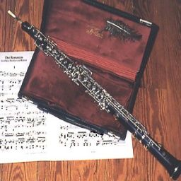
Table 3: Correlation of observed error rates with the cumulative block depth and width parameters
for all ImageNet-X datasets.

                                DATASET                         C. B LOCK D EPTH                        C. B LOCK W IDTH
                                I MAGE N ET                               −0.205                                  −0.511
                                I MAGE N ET-100                           −0.022                                  −0.558
                                I MAGE N ET-10                             0.249                                  −0.457
                                I MAGE N ET-5                               0.51                                  −0.338
                                I MAGE N ET-2                              0.425                                  −0.179

correlations between cumulative block depth/width and the errors on all members of ImageNet-X.
With decreasing number of classes, the correlation coefficients increase for cumulative block depth
and cumulative block width. Although the effect on cumulative block depth is stronger, there is a
significant impact on both parameters. We thus conclude that the number of classes simultaneously
impacts both cumulative block depth and cumulative block width.

                     Insects - :0.95                     MLC 2008 - :0.811                       HAM10000 - :0.608                 Cifar100 - :0.595
         40                                 35.0                                       30
                                                                                                                        50
         30                                 32.5                                       28
                                            30.0                                       26                               40
         20
                                            27.5                                                                        30
         10                                                                            24
                                            25.0
                                                                                       22                               20
          0                                 22.5
               20         40           60           20     30 40 50           60            10       20         30           20          40           60
                    ImageNet-100 error                    ImageNet-10 error                       ImageNet-5 error                 ImageNet-100 error
                     Concrete - :0.106                    Cifar10 - :0.45                        Powerline - :0.294                 Natural - :0.186
                                                                                       50                               80
         1.5
                                            40                                         40
                                                                                                                        60
         1.0                                                                           30
                                            30                                                                          40
                                                                                       20
         0.5
                                                                                       10
                                            20                                                                          20
         0.0                                                                           0
               5      10      15      20           20     30 40 50            60            5      10      15      20         20    30 40 50               60
                     ImageNet-2 error                    ImageNet-10 error                        ImageNet-2 error                 ImageNet-10 error

Figure 8: Test errors of all 500 sampled architectures on target datasets (y-axis) plotted against the
test errors of the same architectures on the ImageNet-X (x-axis). The top 10 performances on the
target dataset are orange, the worst 10 performances red.

We have observed that the number of classes has a profound effect on the APR associated with
ImageNet-X members. It is unlikely that simply varying the number of classes in this dataset is able
to replicate the diversity of APRs present in an array of different datasets. However, it is reasonable
to assume that a dataset’s APR is better represented by the ImageNet-X member closest in terms
of class count, instead of just ImageNet. We thus recreate Figure 4 with the twist of not plotting
the target dataset errors against ImageNet, but against the ImageNet-X variant closest in class count
(see Figure 8). We observe gain in correlation across all datasets, in the cases of MLC2008 or
Cifar10 a quite extreme one. The datasets which have a strong negative correlation with ImageNet
(Powerline, Natural) have slightly (Natural) or even moderately (Powerline) positive correlation to
their ImageNet-X counterparts. A visual inspection shows that the best models on Imagenet-X also
yield excellent results on Powerline and Natural, which was not the case for ImageNet. Table 4
shows the error correlations of all target datasets with ImageNet as well as with their ImageNet-X
counterpart. The move from ImageNet to ImageNet-X more than doubles the average correlation
(from 0.19 to 0.507), indicating that the ImageNet-X family of datasets is capable to represent a much
wider variety of APRs than ImageNet alone.

5   Discussion and Conclusions

ImageNet is not enough. Is it true that models which perform better on ImageNet generally also
perform better on other visual classification tasks? This is the question at the heart of our study. Our
extensive empirical results show that the answer is no. To get an representative estimate of the merits
of a novel architecture, it has to be tested on a variety of datasets which span the whole domain in
which this architecture will be applied.

                                                                                   8
Table 4: Comparison of error correlations between target datasets and ImageNet as well as the closest
ImageNet-X member.

                    DATASET        ρ -I MAGE N ET    ρ -I MAGE N ET-X    D IFFERENCE
                    CONCRETE          0.001               0.106            0.105
                    MLC2008           0.476               0.811            0.335
                    HAM 10000         0.517               0.608            0.091
                    POWERLINE         −0.436              0.294             0.73
                    INSECTS           0.967                0.95            −0.017
                    NATURAL           −0.38               0.186            0.566
                    CIFAR 10          −0.104              0.45             0.554
                    CIFAR 100         0.476               0.595            0.119
                    AVERAGE             0.19              0.507             0.317

Block depth and block width matter. We have identified block depth and block width as key
influence factors on the transferability of an architecture. When designing an architecture for a
practical application, where out of the box models perform poorly, these two dimensions should be
explored first.
Varying the number of classes helps. It is striking how much more accurately the ImageNet-X
family is able to represent the diversity in APRs present in our dataset collection, compared to just
ImageNet by itself. In cases where it is not possible to test an architecture on a variety of different
datasets, it is thus advisable to instead test it on different subsets (with respect to class count) of the
available datasets, similar to how it has become commonplace to test new architectures in multiple
complexity regimes [5, 17].
Future directions. Our study highlights the dangers of optimizing on a single dataset. A future
similar study should shed light on how well the breadth of other domains such as object detection or
speech classification is represented by their most used datasets.
A labeled dataset will always be a biased description of the visual world, due to having a fixed number
of classes and being built with some systematic image collection process. Self-supervised learning of
visual representations [39] could serve as remedy for this issue. Self-supervised architectures could
be fed with a stream completely unrelated images, collected from an arbitrary number of sources in a
randomized way. A comparison of visual features learned in this way could yield a more meaningful
measure of the quality of CNN architectures.
Limitations As with any experimental analysis of a highly complex process such as training a CNN
it is virtually impossible to consider every scenario. We list below three dimensions along which our
experiments are limited together with measures we took to minimize the impact of these limitations.
Data scope: We criticize ImageNet for only representing a fraction of the “visual world”. We are
aware that our dataset collection does not span the entire “visual world” either but went to great
lengths to maximise the scope of our dataset collection by purposefully choosing datasets from
different domains, which are visually distinct.
Architecture scope: We sample our architectures from the large AnyNetX network space. It contains
the CNN building blocks to span basic designs such as AlexNet or VGG as well as the whole ResNet,
ResNeXt and RegNet families. We acknowledge that there are popular CNN components not covered,
however, Radosavovic et al. [36] present ablation studies showing that network designs sourced
from high performing regions in the AnyNetX space also perform highly when swapping in different
originally missing components such as depthwise convolutions [40], swish activation functions [41]
or the squeeze-and-excitation [42] operations.
Training scope: When considering data augmentation and optimizer settings there are almost endless
possibilities to tune the training process. We opted for a very basic setup with no bells an whistles in
general. For certain such aspects of the training, which we assumed might skew the results of our
study (such as training duration, dataset prepossessing etc.), we have conducted extensive ablation
studies to ensure that this is not the case (see sections B.2 and B.7 in the appendix).

                                                    9
Acknowledgments and Disclosure of Funding
This work has been financially supported by grants 25948.1 PFES-ES “Ada” (CTI), 34301.1 IP-ICT
“RealScore” (Innosuisse) and ERC Advanced Grant AlgoRNN nr. 742870. We are grateful to Frank P.
Schilling for his valuable inputs.

References
  [1] Dan C. Ciresan, Ueli Meier, and Jürgen Schmidhuber. Multi-column deep neural networks for image classification. In 2012 IEEE
      Conference on Computer Vision and Pattern Recognition, pages 3642–3649. IEEE Computer Society, 2012.

  [2] Alex Krizhevsky, Ilya Sutskever, and Geoffrey E. Hinton. Imagenet classification with deep convolutional neural networks. In Peter L.
      Bartlett, Fernando C. N. Pereira, Christopher J. C. Burges, Léon Bottou, and Kilian Q. Weinberger, editors, 26th Annual Conference
      on Neural Information Processing Systems, pages 1106–1114, 2012.

  [3] Karen Simonyan and Andrew Zisserman. Very deep convolutional networks for large-scale image recognition. In Yoshua Bengio and
      Yann LeCun, editors, 3rd International Conference on Learning Representations, 2015.

  [4] Rupesh Kumar Srivastava, Klaus Greff, and Jürgen Schmidhuber. Highway networks. CoRR, abs/1505.00387, 2015.

  [5] Kaiming He, Xiangyu Zhang, Shaoqing Ren, and Jian Sun. Deep residual learning for image recognition. In 2016 IEEE Conference
      on Computer Vision and Pattern Recognition, pages 770–778. IEEE Computer Society, 2016.

  [6] Matthew D. Zeiler and Rob Fergus. Visualizing and understanding convolutional networks. In David J. Fleet, Tomás Pajdla, Bernt
      Schiele, and Tinne Tuytelaars, editors, 13th European Conference on Computer Vision, Proceedings, Part I, pages 818–833. Springer,
      2014.

  [7] Saining Xie, Ross B. Girshick, Piotr Dollár, Zhuowen Tu, and Kaiming He. Aggregated residual transformations for deep neural
      networks. In 2017 IEEE Conference on Computer Vision and Pattern Recognition, pages 5987–5995. IEEE Computer Society, 2017.

  [8] Barret Zoph, Vijay Vasudevan, Jonathon Shlens, and Quoc V. Le. Learning transferable architectures for scalable image recognition.
      In 2018 IEEE Conference on Computer Vision and Pattern Recognition, pages 8697–8710. IEEE Computer Society, 2018.

  [9] Joel Hestness, Sharan Narang, Newsha Ardalani, Gregory F. Diamos, Heewoo Jun, Hassan Kianinejad, Md. Mostofa Ali Patwary, Yang
      Yang, and Yanqi Zhou. Deep learning scaling is predictable, empirically. CoRR, abs/1712.00409, 2017.

 [10] Jonathan S. Rosenfeld, Amir Rosenfeld, Yonatan Belinkov, and Nir Shavit. A constructive prediction of the generalization error across
      scales. In 8th International Conference on Learning Representations. OpenReview.net, 2020.

 [11] Jared Kaplan, Sam McCandlish, Tom Henighan, Tom B. Brown, Benjamin Chess, Rewon Child, Scott Gray, Alec Radford, Jeffrey Wu,
      and Dario Amodei. Scaling laws for neural language models. CoRR, abs/2001.08361, 2020.

 [12] Lukas Tuggener, Mohammadreza Amirian, Fernando Benites, Pius von Däniken, Prakhar Gupta, Frank-Peter Schilling, and Thilo
      Stadelmann. Design patterns for resource-constrained automated deep-learning methods. AI, 1(4):510–538, 2020.

 [13] Ilija Radosavovic, Justin Johnson, Saining Xie, Wan-Yen Lo, and Piotr Dollár. On network design spaces for visual recognition. In
      International Conference on Computer Vision, pages 1882–1890. IEEE, 2019.

 [14] Olga Russakovsky, Jia Deng, Hao Su, Jonathan Krause, Sanjeev Satheesh, Sean Ma, Zhiheng Huang, Andrej Karpathy, Aditya Khosla,
      Michael S. Bernstein, Alexander C. Berg, and Fei-Fei Li. Imagenet large scale visual recognition challenge. CoRR, abs/1409.0575,
      2014.

 [15] Alex Krizhevsky, Geoffrey Hinton, et al. Learning multiple layers of features from tiny images. 2009.

 [16] Antonio Torralba and Alexei A. Efros. Unbiased look at dataset bias. In 2011 IEEE Conference on Computer Vision and Pattern
      Recognition, pages 1521–1528. IEEE Computer Society, 2011.

 [17] Andrew G. Howard, Menglong Zhu, Bo Chen, Dmitry Kalenichenko, Weijun Wang, Tobias Weyand, Marco Andreetto, and Hartwig
      Adam. Mobilenets: Efficient convolutional neural networks for mobile vision applications. CoRR, abs/1704.04861, 2017.

 [18] Christian Szegedy, Wei Liu, Yangqing Jia, Pierre Sermanet, Scott E. Reed, Dragomir Anguelov, Dumitru Erhan, Vincent Vanhoucke,
      and Andrew Rabinovich. Going deeper with convolutions. In 2015 IEEE Conference on Computer Vision and Pattern Recognition,
      pages 1–9. IEEE Computer Society, 2015.

 [19] Esteban Real, Alok Aggarwal, Yanping Huang, and Quoc V. Le. Regularized evolution for image classifier architecture search. In The
      Thirty-Third AAAI Conference on Artificial Intelligence, pages 4780–4789. AAAI Press, 2019.

 [20] Hanxiao Liu, Karen Simonyan, and Yiming Yang. DARTS: differentiable architecture search. In 7th International Conference on
      Learning Representations. OpenReview.net, 2019.

 [21] Klaus Greff, Rupesh Kumar Srivastava, Jan Koutník, Bas R. Steunebrink, and Jürgen Schmidhuber. LSTM: A search space odyssey.
      IEEE Trans. Neural Networks Learn. Syst., 28(10):2222–2232, 2017.

                                                                   10
[22] Jasmine Collins, Jascha Sohl-Dickstein, and David Sussillo. Capacity and trainability in recurrent neural networks. In 5th International
Conference on Learning Representations. OpenReview.net, 2017.
[23] Roman Novak, Yasaman Bahri, Daniel A. Abolafia, Jeffrey Pennington, and Jascha Sohl-Dickstein. Sensitivity and generalization in
neural networks: an empirical study. In 6th International Conference on Learning Representations. OpenReview.net, 2018.
[24] Sepp Hochreiter and Jürgen Schmidhuber. Long short-term memory. Neural Comput., 9(8):1735–1780, 1997.
[25] Gábor Melis, Chris Dyer, and Phil Blunsom. On the state of the art of evaluation in neural language models. In 6th International
Conference on Learning Representations,. OpenReview.net, 2018.
[26] Kenji Kawaguchi, Leslie Pack Kaelbling, and Yoshua Bengio. Generalization in deep learning. CoRR, abs/1710.05468, 2017.
[27] Laurent Dinh, Razvan Pascanu, Samy Bengio, and Yoshua Bengio. Sharp minima can generalize for deep nets. In Doina Precup and
Yee Whye Teh, editors, 34th International Conference on Machine Learning, pages 1019–1028. PMLR, 2017.
[28] Chiyuan Zhang, Samy Bengio, Moritz Hardt, Benjamin Recht, and Oriol Vinyals. Understanding deep learning requires rethinking
generalization. In 5th International Conference on Learning Representations. OpenReview.net, 2017.
[29] Benjamin Recht, Rebecca Roelofs, Ludwig Schmidt, and Vaishaal Shankar. Do imagenet classifiers generalize to imagenet? In Ka-
malika Chaudhuri and Ruslan Salakhutdinov, editors, 36th International Conference on Machine Learning, pages 5389–5400. PMLR,
2019.
[30] Jonathan Long, Evan Shelhamer, and Trevor Darrell. Fully convolutional networks for semantic segmentation. In 2015 IEEE Confer-
ence on Computer Vision and Pattern Recognition, pages 3431–3440. IEEE Computer Society, 2015.
[31] Yukang Chen, Tong Yang, Xiangyu Zhang, Gaofeng Meng, Xinyu Xiao, and Jian Sun. Detnas: Backbone search for object detection.
In Hanna M. Wallach, Hugo Larochelle, Alina Beygelzimer, Florence d’Alché-Buc, Emily B. Fox, and Roman Garnett, editors, 32th
Annual Conference on Neural Information Processing Systems, pages 6638–6648, 2019.
[32] Amir Roshan Zamir, Alexander Sax, William B. Shen, Leonidas J. Guibas, Jitendra Malik, and Silvio Savarese. Taskonomy: Disen-
tangling task transfer learning. In Sarit Kraus, editor, International Joint Conference on Artificial Intelligence 2019, pages 6241–6245.
ijcai.org, 2019.
[33] Ali Sharif Razavian, Hossein Azizpour, Josephine Sullivan, and Stefan Carlsson. CNN features off-the-shelf: An astounding baseline
for recognition. In 2014 IEEE Conference on Computer Vision and Pattern Recognition, pages 512–519. IEEE Computer Society,
2014.
[34] Jeff Donahue, Yangqing Jia, Oriol Vinyals, Judy Hoffman, Ning Zhang, Eric Tzeng, and Trevor Darrell. Decaf: A deep convolutional
activation feature for generic visual recognition. In 31th International Conference on Machine Learning, pages 647–655. JMLR.org,
2014.
[35] Simon Kornblith, Jonathon Shlens, and Quoc V. Le. Do better imagenet models transfer better? In 2019 IEEE Conference on Computer
Vision and Pattern Recognition, pages 2661–2671. Computer Vision Foundation / IEEE, 2019.
[36] Ilija Radosavovic, Raj Prateek Kosaraju, Ross B. Girshick, Kaiming He, and Piotr Dollár. Designing network design spaces. In 2020
IEEE Conference on Computer Vision and Pattern Recognition, pages 10425–10433, 2020.
[37] David Freedman, Robert Pisani, and Roger Purves. Statistics (international student edition). Pisani, R. Purves, 4th edn. WW Norton &
Company, New York, 2007.
[38] Thilo Stadelmann, Mohammadreza Amirian, Ismail Arabaci, Marek Arnold, Gilbert François Duivesteijn, Ismail Elezi, Melanie Geiger,
Stefan Lörwald, Benjamin Bruno Meier, Katharina Rombach, et al. Deep learning in the wild. In IAPR Workshop on Artificial Neural
Networks in Pattern Recognition, pages 17–38. Springer, 2018.
[39] Longlong Jing and Yingli Tian. Self-supervised visual feature learning with deep neural networks: A survey. CoRR, abs/1902.06162,
2019.
[40] François Chollet. Xception: Deep learning with depthwise separable convolutions. In 2017 IEEE Conference on Computer Vision and
Pattern Recognition, pages 1800–1807. IEEE Computer Society, 2017.
[41] Prajit Ramachandran, Barret Zoph, and Quoc V. Le. Searching for activation functions. In 6th International Conference on Learning
Representations Workshop Track Proceedings. OpenReview.net, 2018.
[42] Jie Hu, Li Shen, and Gang Sun. Squeeze-and-excitation networks. In 2018 IEEE Conference on Computer Vision and Pattern Recog-
nition, pages 7132–7141. IEEE Computer Society, 2018.
[43] Ç F Özgenel and A Gönenç Sorguç. Performance comparison of pretrained convolutional neural networks on crack detection in
buildings. In ISARC. Proceedings of the International Symposium on Automation and Robotics in Construction, pages 1–8. IAARC
Publications, 2018.
[44] A. S. M. Shihavuddin, Nuno Gracias, Rafael García, Arthur C. R. Gleason, and Brooke Gintert. Image-based coral reef classification
and thematic mapping. Remote. Sens., 5(4):1809–1841, 2013.
11[45] Oscar Beijbom, Peter J. Edmunds, David I. Kline, B. Greg Mitchell, and David J. Kriegman. Automated annotation of coral reef survey
images. In 2012 IEEE Conference on Computer Vision and Pattern Recognition, pages 1170–1177. IEEE Computer Society, 2012.
[46] Philipp Tschandl, Cliff Rosendahl, and Harald Kittler. The HAM10000 dataset: A large collection of multi-source dermatoscopic
images of common pigmented skin lesions. CoRR, abs/1803.10417, 2018.
[47] Ömer Emre Yetgin, Ömer Nezih Gerek, and Ömer Nezih. Ground truth of powerline dataset (infrared-ir and visible light-vl). Mendeley
Data, 8, 2017.
[48] Oskar Liset Pryds Hansen, Jens-Christian Svenning, Kent Olsen, Steen Dupont, Beulhah H. Garner, Alexandros Iosifidis, Benjamin W.
Price, and Toke T. Høye. Image data used for publication "Species-level image classification with convolutional neural network enable
insect identification from habitus images ", November 2019.
[49] Puneet Bansal. Intel image classification. 2018.
[50] Antonio Torralba, Robert Fergus, and William T. Freeman. 80 million tiny images: A large data set for nonparametric object and scene
recognition. IEEE Trans. Pattern Anal. Mach. Intell., 30(11):1958–1970, 2008.
Checklist
1. For all authors...
(a) Do the main claims made in the abstract and introduction accurately reflect the paper’s
contributions and scope? [Yes]
(b) Did you describe the limitations of your work? [Yes] See section 5.
(c) Did you discuss any potential negative societal impacts of your work? [No] Our evalu-
ation focuses on CNN design in general and is not specific enough to any (potentially
harmful) application of image classification.
(d) Have you read the ethics review guidelines and ensured that your paper conforms to
them? [Yes]
2. If you are including theoretical results...
(a) Did you state the full set of assumptions of all theoretical results? [N/A]
(b) Did you include complete proofs of all theoretical results? [N/A]
3. If you ran experiments...
(a) Did you include the code, data, and instructions needed to reproduce the main experi-
mental results (either in the supplemental material or as a URL)? [Yes] It is not possible
for us to add the code in a double-blind way. The final version of this paper will contain
a link to the code and instructions to reproduce every experiment we conducted.
(b) Did you specify all the training details (e.g., data splits, hyperparameters, how they
were chosen)? [Yes] We show the most important training details in our experimental
setup section (see section 4.1). Every last detail will be visible from the actual training
code.
(c) Did you report error bars (e.g., with respect to the random seed after running exper-
iments multiple times)? [Yes] Since we are running experiments on a population of
CNN architectures we get more information out of our computational resources by
growing the population rather than training each architecture multiple times. How-
ever we conducted an ablation study to verify that the level of variability introduced
by changing the CNN architectures is far greater then the variability from random
initialization effects (see section B.3 in the appendix).
(d) Did you include the total amount of compute and the type of resources used (e.g., type
of GPUs, internal cluster, or cloud provider)? [Yes] We mention the number of GPU
hours and used hardware in a footnote of the introduction.
4. If you are using existing assets (e.g., code, data, models) or curating/releasing new assets...
(a) If your work uses existing assets, did you cite the creators? [Yes] All the datasets are
properly cited.
(b) Did you mention the license of the assets? [No] We do not specifically mention
the licenses of the individual dataset, but we mention that they are all sourced form
platforms designed to share scientific data.
12(c) Did you include any new assets either in the supplemental material or as a URL? [Yes]
We will add an URL to a github repository with our code as well as instructions on how
to run it and a download link to all of our trained models. We are not able to do this in
a blind fashion so the URL is omitted from this version.
(d) Did you discuss whether and how consent was obtained from people whose data you’re
using/curating? [No] We only use publicly available data published by the original
authors with the intent for it to be used in research.
(e) Did you discuss whether the data you are using/curating contains personally identifiable
information or offensive content? [No] Most of the datasets we use are of technical
nature and therefore not prone problematic samples. The exceptions—Cifar and
ImageNet—are extremely widely accepted and used.
5. If you used crowdsourcing or conducted research with human subjects...
(a) Did you include the full text of instructions given to participants and screenshots, if
applicable? [N/A]
(b) Did you describe any potential participant risks, with links to Institutional Review
Board (IRB) approvals, if applicable? [N/A]
(c) Did you include the estimated hourly wage paid to participants and the total amount
spent on participant compensation? [N/A]
13A Extended Dataset Description
Concrete [43] contains 40 thousand image snippets
produced from 458 high-resolution images that have Negative Positive
been captured from various concrete buildings on
Concrete
a single campus. It contains two classes, positive
(which contains cracks in the concrete) and negative
(with images that show intact concrete). With 20 thou- CCA Porcill Pavon
sand images in both classes the dataset is perfectly
balanced.
MLC2008
MLC2008 [44] contains 43 thousand image snippets
taken form the MLC dataset [45], which is a subset
of the images collected at the Moorea Coral Reef Clumber spaniel Oboe Suspension bridge
Long Term Ecological Research site. It contains im-
ImageNet
ages from three reef habitats and has nine classes.
The class distribution is very skewed with crustose
coralline algae (CCA) being the most common by far
(see Figure 17 in the Appendix). bkl (benign kera-
nv (melanocytic nevi) me (melanomal) tosis-like lesions)
ImageNet [14] (ILSVRC 2012) is a large scale
dataset containing 1.3 million photographs sourced HAM10000
from flickr and other search engines. It contains 1000
classes and is well balanced with almost all classes
having exactly 1300 training and 50 validation sam-
Negative Positive
Powerline
ples.
HAM10000 [46] ("Human Against Machine with
10000 training images") is comprised of dermato- Ophonus
Clivina collaris Bembidion maritimum schaubergerianus
scopic images, collected from different populations
and by varied modalities. It is a representative collec-
Insects
tion of all important categories of pigmented lesions
that are categorized into seven classes. It is imbal-
anced with an extreme dominance of the melanocytic
nevi (nv) class (see Figure 17 in the Appendix). Sea Street Mountain Glacier Forest Building
Natural
Powerline [47] contains images taken in different
seasons as well as weather conditions from 21 dif-
Cifar10/100
ferent regions in Turkey. It has two classes, positive Cat Dog Truck Ship Deer Bird
(that contain powerlines) and negative (which do not).
The dataset contains 8000 images and is balanced
with 4000 samples per classes. Both classes contain
2000 visible-light and 2000 infrared images. Figure 9: Example images from each dataset.
Images of Cifar10/100 are magnified fourfold,
Insects [48] contains 63 thousand images of 291 in- the rest are shown in their original resolution
sect species. The images have been taken of the (best viewed by zooming into the digital doc-
collection of British carabids from the Natural His- ument).
tory Museum London. The dataset is not completely
balanced but the majority of classes have 100 to 400
examples.
Intel Image Classification [49] dataset (“natural”) is a natural scene classification dataset containing
25 thousand images and 6 classes. It is very well balanced with all classes having between 2.1
thousand and 2.5 thousand samples.
Cifar10 and Cifar100 [15] both consist of 60 thousand images. The images are sourced form the 80
million tiny images dataset [50] and are therefore of similar nature (photographs of common objects)
as the images found in ImageNet, bar the much smaller resolution. Cifar10 has 10 classes with 6000
images per class, Cifar100 consists of 600 images in 100 classes, making both datasets perfectly
balanced.
14Table 5: Top-1 error of reference network implementations [36] for Cifar10.
M ODEL R ES N ET-56 R ES N ET-110 A NY N ET-56 A NY N ET-110
E RROR 5.91 5.23 5.68 5.59
B Additional Ablation Studies
This Chapter contains additional studies not suited for the main text. Most of these studies are designed
to test for possible flaws or vulnerabilities in our experiments and therefore further strengthen the
empirical robustness of our results.
B.1 Stability of Empirical Results on Cifar10
The top-1 errors of our sampled architectures on Cifar10 lie roughly between 18 and 40, which is
fairly poor, not only compared to the state of the art but also compared to performance that can be
achieved with fairly simple models. This calls into question if our Cifar10 results are flawed in a way
that might have lead us to wrong conclusions. We address this by running additional tests on Cifar10
and evaluate their impact on our main results. We get a goalpost for what performance would be
considered good with our style of neural network and training setup by running the baseline code
for Cifar10 published by Radosavovic et al. [36]. Table 5 shows that these baseline configurations
achieve much lower error rates. We aim to improve the error results on Cifar10 in two ways: First
we train our architecture population with standard settings for 200 epochs instead of 30, second we
replaced the standard network stem with one that is specifically built for Cifar10, featuring less stride
and no pooling. Figure 10 shows scatterplots of the errors from all 500 architectures on Cifar10
against the errors on ImageNet and ImageNet-10. We can see that both new training methods manage
to significantly improve the performance with a minimum top-1 error below 10 in both cases. More
importantly can we observe that both new training methods have, despite lower overall error, a
very similar error relationship to ImageNet. The error correlation is even slightly lower than with
our original training (replicated in Figure 10 left row). We can also see that in all three cases the
error relationship can be significantly strengthened by replacing ImageNet with ImageNet-10, this
shows that tuning for individual performance on a dataset does not significantly impact the error
relationships between datasets which further strengthens our core claim.
Cifar10 - :-0.104 Cifar10-tuned-stem - :0.23 Cifar10-200ep - :-0.233
30
40 25 20.0
17.5
20
30 15.0
15 12.5
20 10 10.0
40 60 80 40 60 80 40 60 80
ImageNet error ImageNet error ImageNet error
Cifar10 - :0.45 Cifar10-tuned-stem - :0.619 Cifar10-200ep - :0.139
30
40 25 20.0
17.5
20
30 15.0
15 12.5
20 10 10.0
20 30 40 50 60 20 30 40 50 60 20 30 40 50 60
ImageNet-10 error ImageNet-10 error ImageNet-10 error
Figure 10: The Cifar10 test errors of all 500 architectures plotted against ImageNet (top row) and
ImageNet-10 (bottom row), shown for our original Cifar10 training (left column), training with a
Cifar10 specific stem in the architecture (middle column), and training for 200 epochs, which is
roughly 6 times longer (right column). The plots show that the error correlation with ImageNet-10 is
much larger in all three cases, confirming that optimizing for individual Cifar10 performance does
not alter our core result.
15B.2 Verifying Training Duration
Since we have a limited amount of computational resources and needed to train a vast number of
networks we opted to train the networks up to the number of epochs where they started to saturate
significantly in our pre-studies. As we have seen in section B.1 can the network performance still
improve quite a bit if it is trained for much longer. Even though the improved performances on Cifar10
did not yield any results contradicting the findings of our study, we still deemed it necessary to closer
inspect what happened in the later stages of training and thus performed a sanity check for Cifar10 as
well as the other two datasets that show a negative error correlation with ImageNet—Powerline and
Natural. Figure 11 shows the Cifar10 test error curves of 20 randomly selected architectures over 200
epochs. On the left side we see the same curves zoomed in to epochs 30 to 200. We see that the error
decreases steadily for all architectures, the ranking among architectures barely changes past epoch
30. The relative performance between architectures and not absolute error rates are relevant for our
evaluations, we can therefore conclude that the errors at epoch 30 are an accurate enough description
of an architecture’s power.
Figure 11: Cifar10 test error curves of 20 randomly sampled architectures trained over 200 epochs
(left). The same error curves but cut to epochs 30 to 200.
For Powerline and Natural, we select the five best and five worst architectures respectively and
continue training them for a total of five times the regular duration. Figure 12 shows the resulting
error curves. Both datasets exhibit minimal changes in the errors of the top models. On Natural
we observe clear improvements on the bottom five models but similar to Cifar10 there are very
little changes in terms of relative performance. Powerline exhibits one clear cross-over but for the
remainder of the bottom five models the ranking also stays intact. Overall we can conclude that
longer training does not have a significant effect on the APR of our datasets.
Figure 12: Test error curves of the five best and five worst models on Powerline and Natural,
respectively, when training is continued to epoch 100
B.3 Impact of Training Variability
The random initialization of the model weights has an effect on the performance of a CNN. In an
empirical study it would therefore be preferable to train each model multiple times to minimize this
variability. We opted to increase the size of our population as high as our computational resources
allow, this way we get a large number of measurements to control random effects as well as an error
estimate of a large set of architectures. However, we still wanted to determine how much of the total
variability is caused by training noise and how much is due to changing the architectures. We estimate
16You can also read