LIHOF4: CUBOIDAL DEMAGNETIZING FACTOR IN AN ISING FERROMAGNET
←
→
Page content transcription
If your browser does not render page correctly, please read the page content below
PHYSICAL REVIEW B 102, 144426 (2020)

                           LiHoF4 : Cuboidal demagnetizing factor in an Ising ferromagnet

                        M. Twengström ,1 L. Bovo ,2,3 O. A. Petrenko,4 S. T. Bramwell,2 and P. Henelius1,5
                          1
                            Department of Physics, Royal Institute of Technology, SE-106 91 Stockholm, Sweden
                2
                  London Centre for Nanotechnology and Department of Physics and Astronomy, University College London,
                                         17-19 Gordon Street, London WC1H OAH, United Kingdom
                3
                  Department of Innovation and Enterprise, University College London, 90 Tottenham Court Road, Fitzrovia,
                                                     London W1T 4TJ, United Kingdom
                           4
                             Department of Physics, University of Warwick, Coventry CV4 7AL, United Kingdom
                           5
                             Faculty of Science and Engineering, Åbo Akademi University, 20500 Turku, Finland

                    (Received 17 June 2020; revised 23 September 2020; accepted 23 September 2020; published 19 October 2020)

                 The demagnetizing factor can have an important effect on physical properties, yet its role in determining the
              behavior of nonellipsoidal samples remains to be fully explored. We present a detailed study of the role of spin
              symmetry in determining the demagnetizing factor of cuboids, focusing, as a model example, on the Ising dipolar
              ferromagnet LiHoF4 . We distinguish two different functions: the demagnetizing factor as a function of intrinsic
              susceptibility N (χ ) and the demagnetizing factor as a function of temperature N (T ). For a given nonellipsoidal
              sample, the function N (χ ) depends only on dipolar terms in the spin Hamiltonian, but apart from in the limits
              χ → 0 and χ → ∞, it is a different function for different spin symmetries. The function N (T ) is less universal,
              depending on exchange terms and other details of the spin Hamiltonian. We apply a recent theory to calculate
              these functions for spherical and cuboidal samples of LiHoF4 . The theoretical results are compared with N (χ )
              and N (T ) derived from experimental measurements of the magnetic susceptibility of corresponding samples of
              LiHoF4 , both above and below its ferromagnetic transition at Tc = 1.53 K. Close agreement between theory
              and experiment is demonstrated, showing that the intrinsic susceptibility of LiHoF4 and other strongly magnetic
              systems can be accurately estimated from measurements on cuboidal samples. Our results further show that
              for cuboids, and implicitly for any sample shape, N (χ ) below the ordering transition takes the value N (∞).
              This confirms and extends the scope of earlier observations that the intrinsic susceptibility of ferromagnets
              remains divergent below the transition, in contradiction to the implications of broken symmetry. We discuss the
              topological and microscopic origins of this result.

              DOI: 10.1103/PhysRevB.102.144426

                        I. INTRODUCTION                                  particularly important in the discussion of several phenom-
                                                                         ena that are dominated by long-range interactions, including,
    The demagnetizing energy of a magnetized sample
                                                                         for example, magnetic monopole excitations in the spin ices
presents several intriguing aspects. It plays a crucial role in the
                                                                         [9], topological skyrmionic spin textures [10], and spintronic
analysis of magnetic susceptibility [1,2], realizes a laboratory
                                                                         applications of antiferromagnets [11]. Even the problem of
example of long-range interactions [3], and even mediates
                                                                         how to calculate the demagnetizing factor for shapes beyond
some exotic physics, for example, the complex nonlinear
                                                                         ellipsoids is far from being solved in any general sense: many
response and pattern formation in the intermediate state of
                                                                         years of investigation have yielded some particularly elegant
type-I superconductors [4]. In view of the pioneering work
                                                                         results [12,13], and ongoing work has revealed new surprises.
of Poisson, Maxwell, and others, the “demagnetizing effect”
                                                                         In a recent study [3] we noted an unexpected dependence
may at first sight appear to be a solved problem that belongs
                                                                         of the demagnetizing factor on the microscopic aspects of
to the textbooks, but a closer appraisal of the literature reveals
                                                                         the material for rectangular prismatic samples, in contrast to
that it remains, to this day, a rather rich source of mathematical
                                                                         the long-held expectation that only shape and macroscopic
and practical challenges [5–8]. As far as magnetic materi-
                                                                         susceptibility should be relevant [5]. In this paper we elucidate
als are concerned, demagnetizing effects and corrections are
                                                                         this effect in detail with respect to a real model system: the
                                                                         Ising-like dipolar ferromagnet LiHoF4 .
                                                                             We therefore focus on a fundamental property of mag-
                                                                         netism, namely, the response to a small applied magnetic
Published by the American Physical Society under the terms of the        field: the intrinsic isothermal magnetic susceptibility, χ =
Creative Commons Attribution 4.0 International license. Further          limH →0 ∂M/∂H, where M is the magnetization and H is the
distribution of this work must maintain attribution to the author(s)     internal magnetic field. The susceptibility is a fundamental
and the published article’s title, journal citation, and DOI. Funded     thermodynamic characteristic of a magnetic system, reflecting
by Bibsam.                                                               its microscopic nature and magnetic state. With very careful

2469-9950/2020/102(14)/144426(8)                             144426-1                             Published by the American Physical Society
M. TWENGSTRÖM et al. PHYSICAL REVIEW B 102, 144426 (2020)
measurement, it can reveal surprising properties, as exem-
plified in our recent detection of “special temperatures” in
frustrated magnets [14]. Compared to more local probes of
spin correlations such as neutron scattering or muon relax-
ation, bulk susceptibility measurements offer the advantage
of relative experimental simplicity and precise control of the
experimental environment. However, there are still important
aspects that one must consider in order to obtain a truly
accurate measurement of the intrinsic material susceptibil-
ity. Many materials of recent interest contain high-moment
rare-earth ions leading to a high susceptibility (χ 1) and
consequent strong demagnetizing effects. The state of the sys-
tem can then be defined and determined only after particularly
careful corrections for such effects.
In detail, it is well known that the internal magnetization
and magnetic field of a paramagnetic ellipsoid exposed to
an external magnetic field are uniform within the sample.
The demagnetizing field Hd is given by Hd = −NM, where
M is the magnetization and N is the demagnetizing factor
(more generally, this is a tensor relationship Hdα = −N αβ Mβ ).
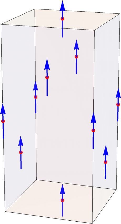
Remarkably, N, as defined in one direction, depends solely on FIG. 1. The conventional unit cell of lithium holmium tetrafluo-
the geometry of the sample and is independent of any under- ride (LiHoF4 ). The red dots represent the holmium ion positions, and
lying material properties. Due to the nature of the long-range the blue arrows indicate the Ising-like spins of LiHoF4 when fully
dipolar interaction, the internal fields become nonuniform magnetized along its principal (c) axis.
for nonellipsoids, and the calculation of the demagnetizing
factors becomes a much more complex task. However, at
an early point it was realized that it is possible to define a with the Ising direction aligned with the principal axis of the
demagnetizing factor for cuboids that depends not only on the tetragonal unit cell containing four Ho3+ ions, with a magnetic
sample geometry but also on the intrinsic susceptibility χ (T ), moment of about 7μB per ion. Due to the relative simplicity of
which leads to the temperature dependence of N [15,16]. the effective model [20], the possibility to dilute the material
Another avenue of research focused on the approximation with nonmagnetic Y3+ ions [21], and its sensitivity to applied
of uniform magnetization, from which useful results were transverse magnetic fields, LiHoF4 has been used in numerous
derived [13,17]. Interestingly, the temperature-dependent N studies on classical and quantum phase transitions [22,23] and
for cuboids has not been applied much in practice, although slow magnetic dynamics [24].
many experiments are performed on cuboids. This is despite The crucial aspect of LiHoF4 for this study is its uniaxial
the fact that the χ dependence of N was calculated [5,6] Ising symmetry, which distinguishes it from the isotropic,
nearly 20 years ago using a finite-element method to solve the multiaxial Ising spin ice compound Dy2 Ti2 O7 used in our
field equations. We and coworkers more recently introduced previous study [3]. In addition, we benefited from the com-
an alternative, iterative microscopic method, along with a mercial availability of LiHoF4 aligned single-crystal samples
brute-force Monte Carlo calculation [3], and the predicted χ cut to a range of shapes and aspect ratios that would have
dependence of N was also supported by direct measurements been challenging to realize in a laboratory (or in house) given
on cuboids of the spin ice compound Dy2 Ti2 O7 . However, the brittle nature of this material. In this investigation we
as already mentioned, in addition to the χ dependence of N, consider spherical, cubic, long, and needle-shaped samples
Ref. [3] further discovered a dependence on the microscopic of LiHoF4 , with dimensions given in Table I. The cuboidal
symmetry of the spin. For example, an isotropic Heisenberg samples were grown, cut, aligned, and polished by Altechna,
spin system or isotropic multiaxial Ising systems such as and we checked their alignment and crystal quality by x-ray
Dy2 Ti2 O7 feature a different N from a uniaxial Ising system.
In this study we test this theory using cuboids of the uniaxial
Ising compound LiHoF4 and find that the theory accounts for TABLE I. Physical dimensions of samples used. Error bars are
the experimentally determined N very well. ∼0.03 mm on dimensions and 1 in the last stated digit on weights.
The last two columns contain the calculated demagnetizing factors
in the limit of zero and infinite susceptibility for each sample.
II. EXPERIMENTAL METHOD
LiHoF4 (see Fig. 1) is an insulating rare-earth dipolar Shape Dimensions (mm) Weight (g) N (χ = 0) N (χ = ∞)
ferromagnet [18]. Due to the low-lying orbitals of the mag- Sphere Ø = 3.8 0.16415 1/3 1/3
netic Ho3+ ions, the dipolar interaction is stronger than the Cube 4.08×3.87 × 4.09 0.36505 0.327 0.274
exchange interaction, and the material orders magnetically at Long 1.95×2.17 × 8.10 0.19235 0.110 0.0751
a relatively low critical temperature of Tc ≈ 1.53 K [19]. Sig- Needle 0.60×0.67 × 8.05 0.01773 0.0363 0.0197
nificant crystal fields lead to a strong uniaxial Ising anisotropy
144426-2LiHoF4 : CUBOIDAL DEMAGNETIZING FACTOR IN … PHYSICAL REVIEW B 102, 144426 (2020)
Laue diffraction. Note that that the “cube” was not perfectly Textbook presentations of the demagnetizing factor em-
cubic, a difference that was accounted for in the analysis. phasize how the homogeneity of the internal field and local
The spherical sample was derived from a sample supplied magnetization for ellipsoids allows one to define a demag-
by Altechna that was further hand cut as in Ref. [14]. It was netizing factor N for a specified crystal axis. This is a fixed
accurately aligned along the crystalline c axis (the easy axis of number for any given ellipsoid: for example, the exact demag-
magnetization) by applying a 7 T magnetic field in a viscous netizing transformation for a sphere (N = 1/3) is
liquid grease at room temperature and then cooling to solidify
the grease. In general, the best estimate for the volume (used 1 1 1
to determine the susceptibility) was calculated through the = − , (2)
weight and the density, ρ = 5.72 g/cm3 . χ χexp, sphere 3
The magnetic susceptibility was studied on different instru-
ments in two temperature regimes, T 1.8 K and T 2 K. where χexp, sphere = ∂M/∂H0 is the experimentally determined
At T 1.8 K, the magnetic moment for each sample was susceptibility and H0 is the uniform applied magnetic field.
measured as a function of temperature using a Quantum De- This is typically contrasted with the case of nonellipsoids,
sign superconducting quantum interference device (SQUID) where neither internal field nor magnetization are uniform,
magnetometer, where the samples were positioned in a cylin- with the consequence that a demagnetizing factor N can no
drical plastic tube to ensure a uniform magnetic environment. longer be defined as a unique, fixed number in the way it
Fields of 15 and 25 Oe were applied, and there was no can for ellipsoids. Nevertheless, for our purposes, it is most
detectable nonlinearity of the susceptibility in this range. important to stress the fact that a temperature-dependent de-
Measurements were performed in the reciprocating sample magnetizing factor N (T ) can still be precisely defined for any
option operating mode to achieve improved sensitivity by sample shape.
eliminating low-frequency noise. For the cuboids we initially To see this, consider an arbitrarily shaped sample, subject
trusted the design specifications and used the cuboid edges as to the field H0 . The incremental magnetic work is μ0 H0 dm,
reference for alignment in the magnetometer (our x-ray study where m = MV is the magnetic moment of the sample of
later showed one sample to have edges that were slightly mis- volume V , which uniquely defines the magnetization M. We
aligned with its crystal axes, as discussed subsequently). By can then write
analogy with Ref. [25], different measurements were made:
low-field susceptibility and field-cooled versus zero-field- 1 1
cooled susceptibility, with no significant differences observed. = − N, (3)
χ χexp, ne
Also, magnetic field sweeps up to several hundred oersteds
at fixed temperature were performed in order to evaluate the
susceptibility accurately, to confirm the linear approximation, where N (T ) is the demagnetizing factor of the nonellipsoidal
and to estimate the absolute susceptibilities, following the (ne) sample, which corresponds to the standard “magnetomet-
method described in our previous work [25]. ric” demagnetizing factor for simple shapes like cylinders or
The magnetic moment at lower temperatures was mea- rectangular prisms.
sured using a different Quantum Design magnetic property It can then be seen by eliminating χ from Eqs. (2) and
measurement system SQUID magnetometer equipped with an (3) that N (T ) is the quantity that precisely maps the tempera-
iQuantum 3 He insert [26]. The applied fields were 50 and ture dependence of the magnetic moment of the nonellipsoid
100 Oe. onto that of the sphere or any arbitrary ellipsoid. Hence, a
Data between the high- and low-temperature regimes have knowledge of N (T ) allows the measurement of χ for any
been compared, in particular in the overlapping region 1.8 sample shape. In the fundamental investigation of magnetic
T 2 K. Without further manipulation, the two sets of data materials, χ is the quantity of interest as it can be calculated,
are in very good agreement with variations of the order of 1%. in principle, from a knowledge of the spin Hamiltonian or
This variation can be attributed to several factors, including simulated numerically using periodic boundaries and Ewald
the uncertainty in the actual field value in each of the two methods. Here, the thermodynamic limit is taken in regards to
instruments (due in part to the presence of small frozen fields the change in the surface term stemming from the fluctuations
in the superconducting coils) and variations in precise sample of the magnetic moments which produce a surface charge. The
positioning within the pickup coils. Here we show only data full derivation was made by de Leeuw et al. [27] using a semi-
below 5 K. classical approach, and a thorough microscopic derivation can
The field, measured in oersteds, and the magnetic moment be found in Ref. [28].
m, measured in emu, were converted into SI units using For a system with inhomogeneous fields, it is therefore
still possible to precisely define N (T ) without making ex-
4π m[emu] plicit reference to the inhomogeneities. They do, however,
χSI = . (1)
H[Oe]V [cm3 ] continue to play a crucial role in determining the numerical
value N (T ) at each temperature. For a given χ , our iterative
method accounts for the inhomogeneity spin by spin and can
III. THEORY OF THE DEMAGNETIZING FACTOR
be implemented on any given spin structure or local spin
The theory that we apply is given in detail in Ref. [3], but symmetry (Ising, XY, Heisenberg) for system sizes up to
it is useful to summarize some of its key aspects here. about N = 106 spins. We supplement it by direct, brute-force,
144426-3M. TWENGSTRÖM et al. PHYSICAL REVIEW B 102, 144426 (2020)
Monte Carlo simulations of the spin Hamiltonian, and in both
cases extrapolate to the thermodynamic limit, N → ∞. In
Ref. [3] we and colleagues showed that the thermodynamic
limit values of N (T ) are in excellent agreement for the two
methods, even though the finite-size corrections are rather
different.
We believe that these methods go beyond previous ap-
proaches in that the viewpoint is no longer mesoscopic (i.e.
“micro”magnetic in the common notation) but, rather, is truly
microscopic and spin Hamiltonian based. Hence, it is more
appropriate for certain fundamental studies, such as that of
spin ice [3] and LiHoF4 , studied here. This conclusion does
not detract from the value of the micromagnetic approaches
for many magnetic problems, and we have demonstrated com-
plete agreement between our approach and that of Chen et al.
[5,6] in the case of cubic spin ice.
Indeed, the works of Chen et al. have revealed many impor-
tant features of the problem: notably, for cylinders (and we can
expect the same for cuboids), as χ → 0, the demagnetizing
field is nonuniform, but the magnetization is uniform [29].
Hence, in that limit, using the results of Ref. [13], the cube
has the same demagnetizing factor as a sphere, N = 1/3. In
the opposite limit, χ → ∞, the roles are reversed, and the
demagnetizing field is uniform (on some mesoscopic scale),
but the magnetization is nonuniform [29]. So for a cube, N
takes a different limiting value, N ≈ 0.27. Our work identifies
aspects of the behavior of the function N (χ ) between these
two limits.
In our method, we first determine the function N (χ ), which
depends only on the definition of the spin degrees of freedom
and their dipole-dipole interactions and, importantly, is inde-
pendent of exchange terms in the spin Hamiltonian. Then,
by substituting χ (T ) into N (χ ), the new function N (T ) is FIG. 2. The experimentally measured susceptibility (top panel)
determined, and it is at this point that the full details of the and inverse susceptibility (bottom panel) as a function of temperature
spin Hamiltonian enter into the problem. Hence, all relevant T for the differently shaped samples of LiHoF4 listed in Table I. The
terms in the spin Hamiltonian affect N (T ), but only dipolar lower plot also shows χ → 0 and χ → ∞ values of N (χ ) from the
tables of Ref. [6].
terms affect N (χ ).
The effect of anisotropy terms in the spin Hamiltonian is
rather subtle. They will, in general, affect the bulk suscepti- IV. RESULTS
bility tensor and, through that, the demagnetizing tensor and In Fig. 2 (top panel) we show the measured low-
demagnetizing factor N (χ ) in a way that is compatible with temperature susceptibility of the different samples and note
the crystal symmetry. For example, spin ice has local Ising that the shape dependence dominates the susceptibility.
spins, but its space symmetry is cubic. Hence, the local Ising The inverse susceptibility, shown in Fig. 2 (bottom panel),
terms are not manifest in the function N (χ ), which is the same is very reminiscent of Fig. 2 in the detailed early study of
as that of other isotropic systems. However, they do strongly Cooke et al. [30]. The low-T plateau in the inverse susceptibil-
affect the temperature dependence of χ (T ) and, through that, ity below the critical temperature of the material is expected
the function N (T ). to occur at the value of the demagnetizing factor N for the
For the uniaxial spin system studied in this paper and for sample (see Sec. V). The low-T susceptibility thus provides
a given sample shape, N (χ ) will be a different function than direct experimental access to the demagnetizing factor for
that of cubic spin ice because the susceptibility tensor has dif- ferromagnets. The estimated χ → 0 and χ → ∞ values of N
ferent symmetry, although it will coincide in the limit χ → 0, [5,6], indicated respectively by color-coded pluses and crosses
where the magnetization becomes homogeneous, and also, it on the graph, are compared to the low-temperature plateau
seems [3], in the limit χ → ∞, where the demagnetizing field of the susceptibility for each sample. The χ → ∞ values are
becomes homogeneous (see above). It is in this rather subtle significantly closer to experiment, a first significant result that
way, where N (χ ) and N (T ) are both affected, but to different we return to below in Sec. V.
degrees, that microscopic effects—in particular the effects of For the spherical sample we would expect the plateau
local spin symmetry—may be revealed in the behavior of the exactly at χ = 1/N = 3, while it is a bit higher, χ = 3.037,
demagnetizing factor for nonellipsoidal samples, such as the possibly due to a deviation from a perfectly spherical shape.
cuboids studied here. The slope in the limit of high temperature should be identical
144426-4LiHoF4 : CUBOIDAL DEMAGNETIZING FACTOR IN … PHYSICAL REVIEW B 102, 144426 (2020)
for all samples since it is related to the Curie constant of
the material. The gradients of the inverse susceptibility in the
4–4.5 K interval are similar for the sphere and cube (0.211
and 0.215, respectively) but higher for the long sample and
needle (0.233 and 0.228, respectively). This discrepancy is
larger than what our theory can account for. We considered
two possible origins of the discrepancy. First, we investigated
a possible misalignment between the local Ising axis and the
long side of the cuboids. A Laue camera measurement showed
the misalignment to be 5◦ and 6◦ for the long and needle
samples, respectively. However, this degree of misalignment
cannot easily explain a 7%–9% error in the susceptibility.
Second, we considered the effect of finite sample dimensions
leading to a systematic error in the assumed point dipole
approximation, as discussed by Stamenov and Coey [31].
Room temperature measurement of palladium foil samples,
shaped to match our LiHoF4 sample dimensions (Table I),
revealed a ∼7% error (on the low side) in the measured
susceptibility of only the long and needle samples. It seems
safe to conclude that the observed discrepancies of 7% and FIG. 3. Temperature dependence of the experimentally derived
9% largely have this origin, with a small contribution from demagnetizing factor N (T ) for the approximate cube of LiHoF4
misalignment. While it would have been ideal to use much (red circles) as well as for the long sample (magenta circles) and
shorter samples, such samples would have also had to be very the needle sample (blue circles). These are compared to theoretical
thin to preserve their aspect ratios, and this would have made predictions (lines with the same color code) specified in the legend.
them very fragile. Hence, rather than use shorter samples, we Our prediction for Ising spins accounts for the experimental data very
accurately, while other predictions fail, except for the needle sample.
make a correction to the susceptibilities, as described below.
If the demagnetizing factor happened to be independent of
temperature, as many studies assume, all the curves in Fig. 2
(bottom) should simply be vertically shifted images of each (χ → 0) theory fails to describe experiment. For the needle
other, as can be deduced from the classical demagnetizing sample, the difference between theories is small, and the data
transformation confirm that the T -independent theory works reasonably well,
1 1 while the sample geometry in this case precluded a reliable
= − N. (4) calculation by our method.
χ χexp
In order to determine N (T ) for the long sample and needle,
However, in Fig. 2, we clearly see that this is not valid for we multiplied the susceptibilities by factors 1.09 and 1.07,
the spherical and cuboidal samples since the curves start to respectively, to ensure that the slope of χ (T ) approaches the
diverge at low temperature. These temperature-dependent de- same high-T limit, which is a physical requirement. As noted
viations from the usual demagnetizing transformation are the above, we believe that the main source of this deviation is a
main subject of this study. correction to the point dipole approximation in the magneti-
Since the demagnetizing factor for the sphere is indepen- zation measurement [31].
dent of the temperature, we can find the intrinsic susceptibility To emphasize the importance of accurate demagnetizing
of the material using Eq. (4) with N = 1/3.037 = 0.3293 in transformations when the susceptibility is large, like it is for
the present case. Using the intrinsic susceptibility, we then many rare-earth-based magnets at low temperature, we show
obtain the temperature-dependent demagnetizing factor N for in Fig. 4 the result of determining the intrinsic material sus-
the other samples using Eq. (4). ceptibility from the measurement on the cube. In black, we
The main result of this study is shown in Fig. 3, where we show the reference intrinsic susceptibility determined from
see the experimentally determined N as a function of T for the sphere, using N = 0.3293. For comparison, we have trans-
the samples of Table I compared to several theoretical predic- formed the measurement on the cube in three different ways:
tions. The upper red circles denote the experimentally derived using the theory for uniaxial Ising spins (red solid line), the
N (T ) for the cubic sample, compared to our calculation for theory for Heisenberg spins (red dotted line), and the fre-
an Ising system (solid line, calculation given in Ref. [3]), quently used approach of assuming the high-susceptibility
the commonly assumed T -independent value of 1/3 (dashed value of N = 1/3 (red dashed line). As Fig. 4 illustrates,
line, equal to N (χ → 0)), and the theoretical prediction for the theory for uniaxial Ising spins reproduces the reference
an isotropic Heisenberg system [3,5,6] (dotted line). It is con- susceptibility very well, while the theory for Heisenberg spins
firmed that the calculation of Ref. [3] is fully consistent with underestimates the susceptibility considerably—by more than
the experimental result, while the T -independent value and 50% at the lowest temperature. This would cause unaccept-
Heisenberg result both differ significantly from it. In Fig. 3 able errors in, say, the determination of a critical exponent
further results are displayed for the long and needle sam- for the transition. Similarly, the T -independent transformation
ples. For the long sample, the agreement between experiment diverges at χexp = 3, which would falsely indicate a critical
and our theory is very satisfactory, while the T -independent temperature of Tc = 1.8 K, well above the actual Tc = 1.53 K.
144426-5M. TWENGSTRÖM et al. PHYSICAL REVIEW B 102, 144426 (2020)
dipolar magnets RCl3 · 6H2 O (R = Dy, Er) [33] and dys-
prosium ethyl sulfate [34] did, indeed, employ ellipsoidal
samples, so there is no reason to doubt their conclusions. Ear-
lier studies on nonellipsoidal samples may contain systematic
errors, but the results presented here show how accurate intrin-
sic susceptibilities can be estimated from magnetization data
on cuboidal samples. These results therefore have practical
relevance to any experimental technique where the demag-
netizing factor needs to be considered: for example, neutron
diffraction, nuclear magnetic resonance (NMR), muon spin
rotation (μSR), x-ray magnetic circular dichroism (XMCD),
and magneto-optical Kerr effect (MOKE), to list a few. How-
ever, it should also be noted that such results for single
crystals do not easily translate through to powder samples:
in a compacted pellet, for example, the demagnetizing field
will depend on both the overall shape and any internal grain
boundaries or voids. Estimating it accurately would be a
difficult, though interesting, challenge. Hence, measurements
FIG. 4. Experimental intrinsic susceptibility of LiHoF4 derived on single-crystal samples, if available, are always preferable
under different assumptions about the behavior of the demagnetizing when demagnetizing effects are large.
factor for the cubic sample. The true value is determined from the Our measurements at temperatures below Tc confirm that
susceptibility of the sphere using N = 0.3293 (black circles), and the magnetic moment of the cuboidal samples remains re-
this is compared with that derived from the cube using several the- markably constant, at the value m = H0V/N (χ = ∞). This
ories: our theory for uniaxial Ising spins (red solid line), the theory may be simply derived by setting the internal field to zero in
for Heisenberg spins (red dotted line), and the commonly used, T - the equation
independent value of N = 1/3 (red dashed line). It can be seen that
the use of an incorrect demagnetizing factor leads to unacceptable
Hint = H0 − NM. (5)
errors in the derived intrinsic susceptibility. The plot also contrasts Indeed, it is a well-known property of many (typically “soft”)
the apparent Tc = 1.80 K implied by the T -independent curve with ferromagnets that was discussed theoretically many years ago
the correct Tc = 1.53 K, corresponding to the divergence of the Ising [35–37]. It appears that the closest to an explanation of this
curve. experimental fact was that found by Wojtowicz and Rayl [36],
who considered a highly idealized model of a toroidal sample,
where a perpendicular ordering field competes with a curling
V. DISCUSSION AND CONCLUSION
mode within the plane of the toroid: in that case, a mean-field
In summary, the demagnetizing transformation for an el- treatment yielded the observed behavior. This is an interesting
lipsoid involves a single number that depends only on sample result as it suggests a topological origin to the experimental
shape. For a nonellipsoidal sample the transformation is still observation of constant moment. However, in the present case
well defined but becomes much more subtle. Taking a cubic of a uniaxial magnet it is difficult to make the same argument
sample as an example, in the small-χ limit, the transforma- as the low-temperature state is not a curling mode but, rather, a
tion is (surprisingly) the same as that of a sphere, N = 1/3, complex domain state. In early studies of several uniaxial sys-
and in the large-χ limit, it reaches a number that does not tems including LiHoF4 (see Ref. [30] and references therein),
depend on any microscopic details of the spin Hamiltonian. it was proposed that domain wall movement is sufficiently free
Between these limits, as we have demonstrated by compar- that domains move so that the average demagnetizing field
ing experiment to microscopic theory, N (χ ) depends on the exactly cancels the applied field. Certainly, if the response
underlying microscopic symmetry of the magnetic moment is confined to the movement of purely macroscopic objects
of the material. In Fig. 3, it is confirmed that the measured (the domain walls), this would be associated with effectively
demagnetizing factor N for the nearly cubic sample of LiHoF4 zero entropy change per spin and hence athermal behavior.
is accurately accounted for by our theory, which takes the If the free energy is equated to the demagnetizing energy
symmetry of the spin and the T -dependence into account, E = (μ0V/2)NM 2 , then χexp = 1/N, as observed.
while the measurement differs from both the T -dependent However, for nonellipsoidal samples, this raises the ques-
result for an isotropic material [3,5,6] and the T -independent, tion as to which demagnetizing factor to use in the calculation
small-χ value. In Fig. 4, we see that this seemingly small of the moment. Our results (Fig. 2, bottom panel) show con-
difference in N has a very significant effect on the final trans- clusively that it is, indeed, the χ = ∞ value of N (χ ), as
formed intrinsic susceptibility of the material, the aim of most calculated here and in Refs. [5,6], rather than the usual χ = 0
susceptibility measurements. value. As predicted in Ref. [38], the paramagnetic fluctuations
It is clear that use of an ellipsoidal sample, where the seem to anticipate the low-temperature domain structure.
temperature-independent demagnetizing factor is known, is a This result strongly indicates that χ = ∞ for all T Tc ,
robust way to accurately determine the intrinsic susceptibility regardless of sample shape. In turn, it raises a certain ambi-
of a material. We note that early measurements of critical guity as to what χ represents in the ordered phase. If χ is
exponents on LiHoF4 [32] and, for example, the rare-earth interpreted as the susceptibility for N = 0, then one has to
144426-6LiHoF4 : CUBOIDAL DEMAGNETIZING FACTOR IN … PHYSICAL REVIEW B 102, 144426 (2020)
admit that it should be finite below Tc because of the broken the critical exponent β (see, for example, Ref. [34]). It is not
symmetry of the ferromagnetic state. On the other hand, if it clear whether this property will precisely survive in the case
is defined as in Fig. 3 to be a property of a sphere (say), then it of a nonellipsoidal sample because even though the internal
can be infinite as a property of the spherical domain state. As field is zero and the magnetic moment is continuous with
the temperature is lowered below Tc , the domain magnetiza- temperature, the magnetization itself is nonuniform even in
tion will increase, and the domain susceptibility will decrease, the high-temperature phase (see Sec. III). Hence, although
consistent with a dipolar ordering transition [22,32], but the corrections to the kink point method may not be very large, it
bulk intrinsic susceptibility will remain infinite. The infinite should be applied with caution when nonellipsoidal samples
susceptibility, or “critical line,” at all temperatures below Tc are used.
is reminiscent of a topologically ordered Kosterlitz-Thouless It is indeed worth emphasizing that the corrections to the
phase [39] or of a soft mode (infinite transverse susceptibility) demagnetizing transformation that we have identified are, of
in an ordered, continuously degenerate system. In view of course, indicative of inhomogeneous fields within the sam-
the Wojtowicz-Rayl argument [36], where the ferromagnetic ple. Such inhomogeneities are likely to be macroscopic, with
transition is accompanied by the appearance of a global topo- details on length scales that are not much shorter than the
logical defect (the winding mode of a torus), and the infinite sample dimensions [40]. Thus, diffuse magnetic neutron scat-
susceptibility as N → 0 does arise from a soft mode, such tering, which measures generalized susceptibilities on rather
analogies are worth considering. A detailed numerical study smaller scales, is not likely to be strongly affected by these
of domain patterns in LiHoF4 revealed a preference for a corrections, but magnetic Bragg scattering will be strongly
structure of parallel (to c) sheets of alternately spin “up” and affected—a fact that will need to be accounted for in neu-
spin “down” [40]. The infinite susceptibility could then reflect tron scattering studies of ordered states. In general, from the
the free motion of smooth or rough domain walls that restore perspective of magnetic moment measurement, field inho-
symmetry (at least locally) between spin-up and spin-down mogeneities represent a correction to be transformed away,
ordered states. There is, indeed, a certain topological character but from a more general perspective, they are an interesting
to the phenomenon as domain walls can be classified as topo- phenomenon in their own right and can be precisely analyzed,
logical defects, and rough ones can even map microscopically as we have illustrated in this paper.
to the Kosterlitz-Thouless phase (although the evidence is that
ACKNOWLEDGMENTS
the long-range interaction suppresses roughness in LiHoF4
[41]). Further investigation of the topological origins of the The simulations were performed on resources provided by
flat susceptibility of ferromagnets would certainly be worth- the Swedish National Infrastructure for Computing (SNIC)
while. at the Center for High Performance Computing (PDC) at
The insights of Ref. [36] further defined the “kink point” the Royal Institute of Technology (KTH). We gratefully ac-
method of measuring the spontaneous magnetization as a knowledge the NVIDIA Corporation for the donation of GPU
function of temperature. At the “kink” temperature Tk where resources. M.T. was supported by Stiftelsen Olle Engkvist
the magnetic moment becomes “flat,” the vanishing of the Byggmästare (Grant No. 187-0013) with support from Mag-
internal field, coupled with the continuity of the magnetic nus Bergvalls Stiftelse (Grant No. 2018-02701). L.B. was
moment versus temperature curve, suggests that the sponta- supported by the Leverhulme Trust through the Early Career
neous magnetization Ms (Tk ) is given by Ms (Tk ) = H0 /N. By Fellowship programme (Grant No. ECF2014-284). The au-
varying H0 , one can determine the function Ms (T ) and hence thors declare no competing financial interests.
[1] E. C. Stoner, Philos. Mag. 36, 803 (1945). [12] G. Rowlands, J. Magn. Magn. Mater. 118, 307 (1993).
[2] J. A. Osborn, Phys. Rev. 67, 351 (1945). [13] P. Rhodes and G. Rowlands, Proc. Leeds Philos. Lit. Soc., Sci.
[3] M. Twengström, L. Bovo, M. J. P. Gingras, S. T. Bramwell, and Sec. 6, 191 (1954).
P. Henelius, Phys. Rev. Mater. 1, 044406 (2017). [14] L. Bovo, M. Twengström, O. A. Petrenko, T. Fennell, M. J. P.
[4] R. Prozorov, R. W. Giannetta, A. A. Polyanskii, and G. K. Gingras, S. T. Bramwell, and P. Henelius, Nat. Commun. 9,
Perkins, Phys. Rev. B 72, 212508 (2005). 1999 (2018).
[5] D.-X. Chen, E. Pardo, and A. Sanchez, IEEE Trans. Magn. 38, [15] J. Würschmidt, Z. Phys. 12, 128 (1923).
1742 (2002). [16] F. von Stäblein and H. Schlechtweg, Z. Phys. 95, 630 (1935).
[6] D.-X. Chen, E. Pardo, and A. Sanchez, IEEE Trans. Magn. 41, [17] R. I. Joseph and E. Schlömann, J. Appl. Phys. 36, 1579
2077 (2005). (1965).
[7] M. Beleggia, M. De Graef, and Y. T. Millev, Philos. Mag. 86, [18] M. J. P. Gingras and P. Henelius, J. Phys.: Conf. Ser. 320,
2451 (2006). 012001 (2011).
[8] G. Di Fratta, Proc. R. Soc. A 472, 20160197 (2016). [19] G. Mennenga, L. J. deJongh, and W. J. Huiskamp, J. Magn.
[9] C. Castelnovo, R. Moessner, and S. L. Sondhi, Nature 451, 42 Mater 44, 59 (1984).
(2008). [20] P. B. Chakraborty, P. Henelius, H. Kjønsberg, A. W. Sandvik,
[10] N. Nagaosa and Y. Tokura, Nat. Nanotechnol. 8, 899 (2013). and S. M. Girvin, Phys. Rev. B 70, 144411 (2004).
[11] T. Jungwirth, J. Sinova, A. Manchon, X. Marti, J. Wunderlich, [21] D. H. Reich, T. F. Rosenbaum, and G. Aeppli, Phys. Rev. Lett.
and C. Felser, Nat. Phys. 14, 200 (2018). 59, 1969 (1987).
144426-7M. TWENGSTRÖM et al. PHYSICAL REVIEW B 102, 144426 (2020)
[22] J. A. Griffin, M. Huster, and R. J. Folweiler, Phys. Rev. B 22, [31] P. Stamenov and J. M. D. Coey, Rev. Sci. Instrum. 77, 015106
4370 (1980). (2006).
[23] D. Bitko, T. F. Rosenbaum, and G. Aeppli, Phys. Rev. Lett. 77, [32] P. Beauvillain, J. P. Renard, I. Laursen, and P. J. Walker, Phys.
940 (1996). Rev. B 18, 3360 (1978).
[24] A. Biltmo and P. Henelius, Nat. Commun. 3, 857 (2012). [33] E. Lagendijk and W. J. Huiskamp, Physica (Amsterdam) 65,
[25] L. Bovo, L. D. C. Jaubert, P. C. W. Holdsworth, and S. T. 118 (1973).
Bramwell, J. Phys.: Condens. Matter 25, 386002 (2013). [34] R. Frowein and J. Kotzler, Z. Phys. B 25, 279 (1976).
[26] N. Shirakawa, H. Horinouchi, and Y. Yoshida, J. Magn. Magn. [35] A. Arrott, Phys. Rev. Lett. 20, 1029 (1968).
Mater. 272–276, e149 (2004). [36] P. J. Wojtowicz and M. Rayl, Phys. Rev. Lett. 20, 1489
[27] S. W. de Leeuw, J. W. Perram, and E. R. Smith, Proc. R. Soc. (1968).
London, Ser. A 373, 27 (1980). [37] R. B. Griffiths, Phys. Rev. 188, 942 (1969).
[28] J. W. Perram and E. R. Smith, J. Stat. Phys. 46, 179 (1987). [38] W. Wasilewski, Phys. Lett. A 84, 80 (1981).
[29] D.-X. Chen, J. A. Brug, and R. B. Goldfarb, IEEE Trans. Magn. [39] J. M. Kosterlitz and D. J. Thouless, J. Phys. C: Solid State Phys.
27, 3601 (1991). 6, 1181 (1973).
[30] A. H. Cooke, D. A. Jones, J. F. A. Silva, and M. R. Wells, [40] A. Biltmo and P. Henelius, Europhys. Lett. 87, 27007 (2009).
J. Phys. C 8, 4083 (1975). [41] G. I. Mias and S. M. Girvin, Phys. Rev. B 72, 064411 (2005).
144426-8You can also read