LUCI onboard Lagrange, the Next Generation of EUV Space Weather Monitoring
←
→
Page content transcription
If your browser does not render page correctly, please read the page content below

submitted to Journal of Space Weather and Space Climate
                                               c The author(s) under the Creative Commons Attribution 4.0 International License (CC BY 4.0)

                                                LUCI onboard Lagrange, the Next Generation of
                                                       EUV Space Weather Monitoring
arXiv:2009.04788v1 [astro-ph.SR] 10 Sep 2020

                                                 M.J. West1,2,? , C. Kintziger3 , M. Haberreiter4 , M. Gyo4 , D. Berghmans1 , S.
                                                       Gissot1 , V Büchel4 , L. Golub5 , S. Shestov1,6 , and J.A. Davies7

                                                  1   Royal Observatory of Belgium, Ringlaan -3- Av. Circulaire, 1180 Brussels, Belgium
                                                  2   Southwest Research Institute, 1050 Walnut Street, Suite 300, Boulder, CO 80302, USA
                                                  3   Centre Spatial de Liège, Université de Liège, Av. du Pré-Aily B29, 4031 Angleur, Belgium
                                                  4   Physikalisch-Meteorologisches Observatorium Davos, World Radiation Center, 7260, Davos
                                                      Dorf, Switzerland
                                                  5   Harvard Smithsonian CfA, HEA MS 58 60, Garden Str, Cambridge, MA, USA
                                                  6   Lebedev Physical Institute, Leninskii prospekt, 53, 119991 Moscow, Russia
                                                  7   Rutherford Appleton Laboratory, Harwell Campus, Oxfordshire, OX11 0QX, UK

                                                                                             ABSTRACT

                                                  LUCI (Lagrange eUv Coronal Imager) is a solar imager in the Extreme UltraViolet (EUV) that is
                                                  being developed as part of the Lagrange mission, a mission designed to be positioned at the L5
                                                  Lagrangian point to monitor space weather from its source on the Sun, through the heliosphere,
                                                  to the Earth. LUCI will use an off-axis two mirror design equipped with an EUV enhanced active
                                                  pixel sensor. This type of detector has advantages that promise to be very beneficial for monitoring
                                                  the source of space weather in the EUV. LUCI will also have a novel off-axis wide field-of-view,
                                                  designed to observe the solar disk, the lower corona, and the extended solar atmosphere close to
                                                  the Sun-Earth line. LUCI will provide solar coronal images at a 2-3 minute cadence in a pass-band
                                                  centred on 19.5 nm. Observations made through this pass-band allow for the detection and mon-
                                                  itoring of semi-static coronal structures such as coronal holes, prominences, and active regions;
                                                  as well as transient phenomena such as solar flares, limb Coronal Mass Ejections (CMEs), EUV
                                                  waves, and coronal dimmings. The LUCI data will complement EUV solar observations provided
                                                  by instruments located along the Sun-Earth line such as PROBA2-SWAP, SUVI-GOES and SDO-
                                                  AIA, as well as provide unique observations to improve space weather forecasts. Together with a
                                                  suite of other remote-sensing and in-situ instruments onboard Lagrange, LUCI will provide science
                                                  quality operational observations for space weather monitoring.

                                                  Key words. Instrumentation: detectors – Space vehicles: instruments – Telescopes; Sun: corona;
                                                  Sun: UV radiation

                                                                                                                                                         1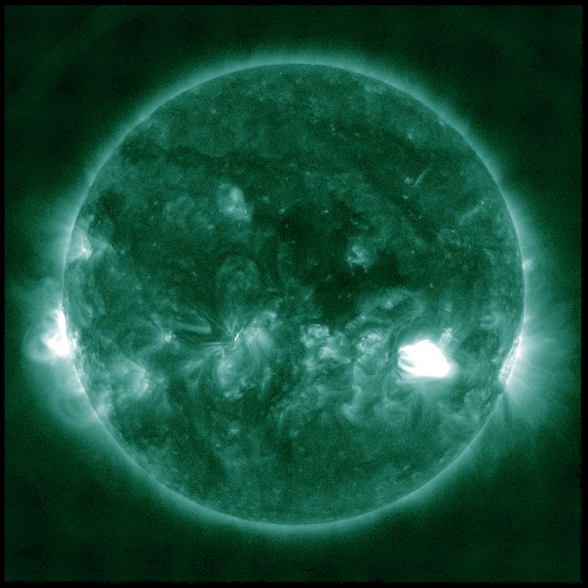
West et al.: The LUCI Instrument

1. Introduction

Space weather is manifest in many forms, from the background solar wind and the interplanetary
magnetic field carried by the solar wind plasma, to more short-lived energetic events including
Coronal Mass Ejections (CMEs), the sudden release of radiation into space by solar flares, and
Solar Energetic Particles (SEPs) generated by CME driven shocks and flares. Each event can af-
fect the near-Earth system and human life in different ways; SEPs can trigger solar particle events
throughout the solar system, where-as the magnetic fields and energetic particles in eruptions and
the solar wind can induce geomagnetic storms, ionospheric disturbances and scintillation of radio
signals (see Hapgood (2017) for a thorough review). Due to its impacts, especially on ever in-
creasing space-based sensitive equipment, space weather monitoring and forecasting have become
increasingly important.
   The ESA Space Safety Program (S2P) Space WEather (SWE) segment has been set up to sup-
port the utilisation and access of space through the provision of timely and accurate information
regarding the space environment, particularly regarding hazards to infrastructure in orbit and on
the ground. An important part of the S2P space weather network is space-based instrumentation,
where, from the vantage point beyond the Earth’s protective atmosphere, space-based instruments
can monitor the local environment through in-situ monitoring instruments, as well as make remote
sensing observations to anticipate the possible future effects of space weather.
   Most space weather monitoring instrumentation is based along the Sun-Earth line, principally
in Earth orbit and at the L1 Lagrangian point, which is upstream in the solar wind with re-
spect to the Earth, providing us with information about space weather coming towards the Earth.
Another important location identified for space weather monitoring is the L5 Lagrangian point (e.g.
Gopalswamy et al., 2011), located approximately 60 degrees behind the Earth in its orbit. The left
panel of Figure 1 shows the positions of the 5 Lagrangian points, from a view point above the solar
north pole. The Lagrangian points represent positions of relative stability for satellites, where the
Sun and Earth’s combined gravitational and centrifugal pulls balance.
   An L5 based observatory offers several observational benefits for space weather monitoring. For
example, it allows us to monitor eruptions from the side, providing more accurate measurements
of the direction and speed of phenomena moving towards the Earth, which would otherwise be
observed coming directly towards the observer. From the Earth perspective, eruptions emerging
from near solar disk centre are of most interest, as it’s these events that will eventually reach the
Earth. However, they’re observed as expanding Halos, making it difficult to measure the speed and
size (Gopalswamy et al., 2010), where a wide slow CME may be perceived as a fast narrow CME
or vice versa. The blue ice-cream cone shape in the right panel of Figure 1 represents such an Earth
directed eruption.
   When monitoring the sources of space weather on the Sun, increasing the size of your view
is important, as is increasing the amount of time you can monitor a potential source before it is
Earth effective. The red arrow in Figure 1 indicates the direction of solar rotation and highlights the
potential for an imager to observe the solar disk before it is Earth orientated. The right panel of 1
indicates the different viewing perspectives of the Sun from an observatory positioned at the L1 and

?   Corresponding author: Matthew J. West e-mail: mwest@boulder.swri.edu

                                                                                                     2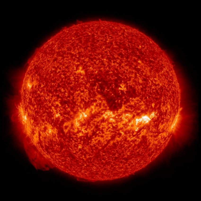
West et al.: The LUCI Instrument

Fig. 1. Left: The position of the 5 Lagrangian points relative to the Sun and Earth system from a solar north
perspective, where the red arrow indicates the direction of solar rotation. Right: The different perspectives of
the Sun from the L1 and L5 points, represented by red and green lines respectively. The blue ice-cream cone
shape represents an Earth directed eruption.

L5 points, represented by red and green lines respectively. An L5 based observatory would extend
our view of the Sun by an additional 60 degrees.
   The source of most space weather can be directly attributed to solar phenomena observed in the
lower solar atmosphere, on the solar disk and out to several solar radii off the limb. Instruments
imaging the Sun through Extreme UltraViolet (EUV) pass-bands provide us with one of the best
means of observing this region, allowing us to observe the region through a broad range of tem-
peratures (e.g. EIT on SoHO Delaboudinière et al., 1995). One example of such an instrument is
the Sun Watcher using Active Pixel System detector and Image Processing (SWAP; Seaton et al.
(2013a); Halain et al. (2013)) EUV telescope on PROBA2 (Hochedez et al., 2006), whose oper-
ations have been funded through the ESA S2P program for several years. SWAP is a small EUV
telescope that images the solar corona, through a pass-band focussed on the Fe IX/X emission lines
(corresponding to a 17.4 nm EUV pass-band). EUV observations allow us to image the lower solar
atmosphere at temperatures ranging between several thousand and several million K. The funda-
mental building block of the solar atmosphere is the Sun’s magnetic field which permeates the solar
atmosphere, and it’s at temperatures observed through EUV pass-bands that we can see magnetic
structures highlighted by the hot plasma trapped on them.
  Figure 2 shows two images of the solar atmosphere, from 2014-Jan-01 at 00:10 UT (top left)
and 2020-Jan-01 at 00:10 UT (top right), taken with the Atmospheric Imaging Assembly (AIA
Lemen et al., 2012) on the Solar Dynamics Observatory (SDO) in the 19.3 nm pass-band. The
AIA 19.3 nm pass-band primarily observes the Sun at temperatures around 1.6 × 10⁶ K. At this
temperature we can see the rich menagerie of solar structures, including hot bright active regions
and the relatively cool coronal holes. By comparing the two images in Figure 2 we can also see
the stark differences between the structure of the Sun at solar maximum (left) and solar minimum

                                                                                                              3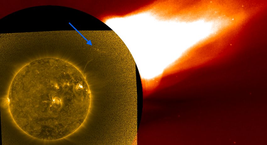
West et al.: The LUCI Instrument

Fig. 2. Top: Two representative images of the Sun from the AIA instrument on SDO, through the 19.3 nm
pass-band, from solar maximum (left; 2014-Jan-01) and solar minimum (right; 2020-Jan-01). Bottom:
Highlights several different manually identified regions that can be identified in the corresponding images
above, such as active regions (green), equatorial coronal holes (blue), filament channels (red), and polar
coronal holes (yellow).

(right), where the solar disk transforms from one being peppered with active regions, indicating
regions of intense magnetic activity, to a more placid one dominated by quiet sun regions, with
two well defined polar coronal holes. The solar activity of interest to the space weather community
ranges from long-lived (semi-static) structures, with the aim of trying to anticipate when they may
produce activity at the Earth, to more dynamic events. Long-lived structures include coronal holes,

                                                                                                         4
West et al.: The LUCI Instrument

active regions and prominences (filaments). More dynamic events, which are often intrinsically
related to the long-lived structures, include flares and eruptions. EUV instruments, when combined
with coronagraphic white-light observations from instruments such as LASCO (Brueckner et al.,
1995) onboard the Solar and Heliospheric Observatory (SoHO), allow space weather observers to
monitor solar activity from the solar surface out to several solar radii.
   The Lagrange mission is being developed under the S2P, SWE segment, to place an operational
space weather monitor at the L5 point with the express purpose of monitoring solar activity and
space weather along the Sun-Earth line. The Lagrange mission, in its current form, contains four
remote-sensing optical instruments and five in-situ instruments to analyse the Sun, inner helio-
sphere, energetic particle streams, and the ambient solar wind conditions. One of those instru-
ments will be the Lagrange eUv Coronal Imager (LUCI), which is a solar imager in the Extreme
UltraViolet (EUV).
   Several studies have used observations made by the Sun Earth Connection Coronal and
Heliospheric Investigation (SECCHI) package (Howard et al., 2008) from NASA’s Solar Terrestrial
Relations Observatory (STEREO Kaiser et al., 2008) mission, when they were positioned close to
the L4 and L5 points, to highlight the advantages of monitoring space weather from close to this
position. Bailey et al. (2020) showed that predicting the minimum Dst at Earth can be improved
with an L5 based observatory, and Rodriguez et al. (2020) showed forecasts of CME arrival times
are improved with L5 observational input. Byrne et al. (2010), using observations from when the
STEREO satellites were near quadrature with the Earth (86.7◦ separation), made three-dimensional
reconstructions of a CME to determine an accurate arrival time of the eruption at the Lagrangian L1
point, highlighting the efficiency of forecasting with instrumentation off the Sun-Earth line. This
work not only utilised white light instrumentation (coronagraphs and Heliospheric Imagers (HI;
Eyles et al., 2009)), but also EUV observations to help determine the direction of propagation. The
work also highlights that significant acceleration occurs lower down in the solar atmosphere, in
regions most typically observed with large field-of-view (FOV) EUV imagers.
   The LUCI imager is being designed to image the solar atmosphere in the EUV from the L5
Lagrangian point, in an operational capacity with the interests of space weather forecasters in mind.
In Section 2 of this article we review the different phenomena required to be observed by an EUV
imager for space weather services and science. In Section 3 we present the current design of the
instrument, highlighting some of the technical innovations and heritage incorporated into the mis-
sion, and section 4 presents a discussion on the rationale behind those decisions, and the logistics
of operating an EUV imager in the harsh and remote environment of the L5 point.

2. Space Weather EUV Observations

The Sun is the source of all space weather that could impact the Earth, other planetary bodies and
human infrastructure. It therefore needs careful observation to help understand upcoming risks and
to forecast the impact. Although the origins of space weather are intrinsically linked to the magnetic
fields formed deep in the Sun’s unobservable convection zone and tachocline, it’s the manifestation
in the solar atmosphere that needs to be monitored, in particular in the lower and middle corona. It’s
in these regions where the motions from within the Sun, combined with large magnetic Reynolds
numbers found in the corona, can cause current sheets to build up, and energy to be liberated through

                                                                                                    5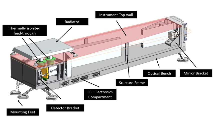
West et al.: The LUCI Instrument

the process known as magnetic reconnection. The energy released, and the reconfiguration of the
magnetic fields can result in some of the most spectacular space weather events.
   The corona is observed to be highly inhomogeneous, which is directly attributed to the magnetic
field. In general the solar atmosphere can be separated into open and closed field regions. The closed
field regions are predominantly made up of quiet sun regions and active regions, which are made
up of a series of magnetic flux tubes, or loop structures, piercing the photosphere from below. Open
field regions trace out magnetic fields that close deep in the heliosphere creating an open appearance
on the Sun.
   The solar atmosphere is best observed in the EUV portion of the electromagnetic spectrum, where
hot plasmas ranging in temperature from several thousand to several million Kelvin (K) highlight
magnetic structures permeating the region. Due to the range in temperatures and densities of differ-
ing structures in the solar atmosphere, observations are filtered into pass-bands, characterized by a
limited number of spectral lines. The AIA instrument hosts the largest selection of pass-bands on
a single instrument, covering temperatures from chromospheric to coronal regions. Figure 3 shows
the Sun in six of AIA’s pass-bands, where the top row shows the 30.4 nm (pass-band peak tem-
perature: 5 × 10⁴ K; primary pass-band ions: He II), 17.1 nm (6.3 × 10⁵ K; Fe IX), and 21.1 nm
(2 × 10⁶ K; Fe XIV) pass-bands, and the bottom row shows the 33.5 nm (2.5 × 10⁶ K; Fe XVI),
9.4 nm (6.3 × 10⁶ K; Fe XVIII), 13.1 nm (4 × 10⁵ & 1.0 × 10⁷ K; Fe VIII, XXI) pass-bands. These
images can be directly compared with the left panel of Figure 2, which shows an image from the
19.3 nm (1.6 × 10⁶ & 1.6 × 10⁷ K; Fe XII, XXIV) pass-band acquired at a similar time. To say
individual pass-bands only observe specific features is disingenuous as many of the coronal struc-
tures are multi-thermal and some pass-bands observe broad temperature ranges, through multiple
emission lines. However, each of the pass-bands was originally chosen to highlight different struc-
tures and regions of the solar atmosphere, such as: the 30.4 pass-band observes the chromosphere
and transition region, 17.1 the quiet corona and upper transition region, 19.3 the corona and hot
flare plasma, 21.1 and 33.5 active regions, 9.4 the flaring corona, and 13.1 the transition region and
flaring corona (see Table 1 in Lemen et al. (2012)).
   Teams monitoring space weather are primarily interested in understanding and forecasting when
events will happen, and if the events will impact the Earth directly or indirectly. The monitoring can
be broadly grouped into two categories, the monitoring of semi-static structures and of dynamic
structures. Semi-static structures are long-lived, persisting from days to multiple solar rotations,
and include: coronal holes, active regions, and prominences (filaments). Whereas dynamic struc-
tures are more short lived, lasting for minutes to hours, and include: flares, CMEs and their related
phenomena.
   In EUV observations, coronal holes appear as regions of lower emission in contrast to the sur-
rounding corona, due to the lower temperature and density of the plasma observed there. At pho-
tospheric and chromospheric temperatures coronal holes are almost indistinguishable from the sur-
rounding corona, however they can begin to be distinguished when the observing pass-band temper-
ature exceeds about 105 K. Coronal holes come in two varieties: polar and transient. Polar coronal
holes are more persistent, emerging in the polar regions around solar minimum and can persist for
many years. In contrast, equatorial (transient) coronal holes (Rust, 1983; Kahler and Hudson, 2001)
can occur anywhere on the Sun, but are more commonly located around the equatorial regions.
They’re generally more short lived but can still persist for several solar rotations. In the right panel
of Figure 2, two polar coronal holes can be seen capping the top and bottom of the Sun. In the left

                                                                                                      6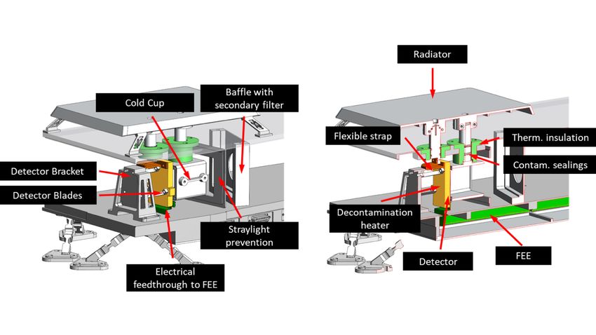
West et al.: The LUCI Instrument

Fig. 3. The Sun observed in six of the AIA imager’s pass-bands on 2014 Jan 01. The top panels (from left
to right) correspond to the pass-bands: 30.4 nm, 17.1 nm, 21.1 nm; The bottom row corresponds to: 33.5 nm,
9.4 nm, 13.1 nm. These can be compared to the left panel of Figure 2, which shows the 19.3 nm pass-band
from AIA at a similar same time.

panel, a large equatorial coronal hole can be seen near disk centre. They are classed as regions of
open magnetic field, and allow plasma to flow away from the Sun relatively unimpeded, creating
High Speed Streams (HSSs) in the solar wind. These HSSs can interact with the relatively slow am-
bient solar wind, creating compression regions, known as Co-rotating Interaction Regions (CIRs).
See Vršnak et al. (2007a) and Vršnak et al. (2007b) for a thorough review on coronal holes and
HSSs. With an Earth orientation, HSSs and their associated CIRs can enhance geomagnetic activ-
ity, the severity of which is dependent on the speed of the stream and the direction of the underlying
interplanetary magnetic field. As a consequence the emergence, growth, and development of coro-
nal holes are a main source of interest for teams monitoring space weather, and EUV observations
of coronal holes are used to help forecast the arrival of HSSs and CIRs.
   Solar prominences, labelled filaments when seen on the solar disk, are arcade-like-structures
seen in absorption at coronal temperatures, as they are made of cool (7 × 10³ ≤ T ≤ 2 × 10⁴ K)
dense material, probably of chromospheric origin. They can be seen as thin dark braided lines in
several pass-bands with a cooler component, and are best seen at chromospheric temperatures, such
as those seen in the 30.4 nm pass-band of AIA (see the top left panel of Figure 3). Prominences
can be found anywhere on the Sun, but they’re often found adjacent to polar coronal holes and

                                                                                                        7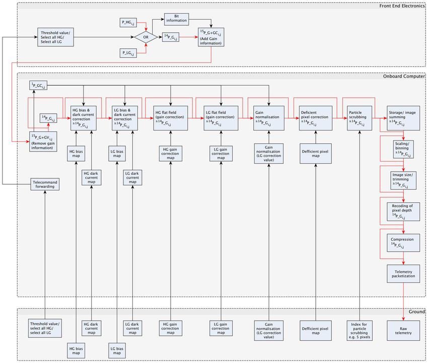
West et al.: The LUCI Instrument

active regions. The number of prominences changes with the solar cycle, with more being seen
near solar maximum. Prominences can remain stable for several solar rotations, before becoming
destabilised and possibly erupting (van Driel-Gesztelyi and Culhane, 2009) leading to some of the
most spectacular eruptions observed. The activation is not fully understood, making forecasts of
their eruption challenging. There’s some evidence that increased motion inside the foot points can
be a precursor to an eruption (Ofman et al., 1998) and therefore careful monitoring is required.
Monitoring the formation of a prominence and its life cycle is another key EUV observable. See
Parenti (2014) for a thorough review of solar prominences.

   Active regions are regions of intense magnetic activity; the concentration of magnetic flux emer-
gence, cancellation, and magnetic reconnection, in these regions releases significant amounts of
energy, directly and indirectly heating the regions to temperatures in excess of 107 K. The result-
ing high-density multi-thermal plasma causes them to emit over a broad spectrum, the emission
coming from a myriad of closed magnetic loop structures that make up the active region. They are
therefore seen in all EUV pass-bands as regions of bright loops (see Figures 2 and 3). The constant
reorganisation of the magnetic topology not only leads to a localised release of energy, but it can
also produce more dramatic events that are of interest to space weather forecasters, including flares
and eruptions. As a consequence active regions are monitored extensively for evidence of upcoming
activity. Precursors to activity have been studied extensively; Zhukov (2005) showed that regions
exhibiting excessive shear and twist are more eruption productive, whereas Lee et al. (2012) found
that active region size is a good indicator of potential flare strength, with larger flares occurring in
larger active regions. The decay phase in certain regions can also lead to increased flaring activity
(e.g. Su et al., 2009). As a consequence, monitoring the emergence, development (e.g. shape) and
subsequent decay of an active region, is paramount. See Toriumi and Wang (2019) for a review of
active regions and their related phenomena.

   Solar flares are one of the most prominent short-lived events monitored by the space weather
community, as they produce intense radiation and can produce streams of high energy particles (so-
lar proton events), which can be harmful to spacecraft and astronauts. They effect all layers of the
solar atmosphere and are observed at wavelengths ranging from radio waves to gamma rays, and
are therefore seen in all EUV pass-bands. Flares can occur anywhere on the Sun, but are generally
associated with regions of complex magnetic topology, such as active regions, and it’s in these re-
gions where the largest flares are observed. The frequency varies with the solar cycle, from several
per day at solar maximum to less than one a week at solar minimum. Flares occur when local mag-
netic fields reconnect, releasing stored magnetic energy and accelerating charged particles. These
particles interact with the plasma medium heating it to tens of millions of K, which in turn can lead
to processes such as chromospheric evaporation which can heat coronal loops (Cargill et al., 1995).
The evolution of how a flare occurs has been largely laid out in a standard model, which is credited
to Carmichael (1964), Sturrock (1966), Hirayama (1974) and Kopp and Pneuman (1976), called the
CSHKP model. The model has been built on and improved by numerous authors, developing into
the Flux Cancellation or the Catastrophe model (see e.g. Lin and Forbes (2000) and Lin (2004)).
See Benz (2017) for a thorough review of solar flare observations. Determining the occurrence of a
flare is not well understood, however there is some correlation with the magnetic complexity of the
source region. As the radiation from flares can reach Earth within minutes, and the exact cause is
unknown, forecasts are generally probabilistic, and depend on evidence of previous flaring activity.

                                                                                                      8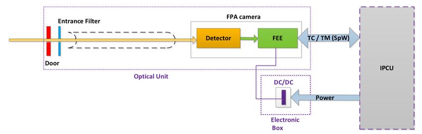
West et al.: The LUCI Instrument

   Solar flares are sometimes accompanied by CMEs, which are eruptions of magnetized plasma
into interplanetary space, and are observed as some of the most dramatic solar phenomena. It is
now generally believed that flares and CMEs are two manifestations of a single magnetically-driven
mechanism (Webb and Howard, 2012). Alongside flares, CMEs are of major concern to teams mon-
itoring space weather as they can trigger severe geomagnetic storms. They’re generally produced
from erupting prominences and from magnetic reconnection in active regions. Although CMEs
have been studied for decades, the exact mechanism responsible for their initiation is still under
debate, and different eruptions may be produced by different mechanisms. Popular models include
the Breakout model (e.g. Antiochos et al., 1999), internal tether-cutting reconnection models (e.g.
Moore et al., 2001), general flux cancellation models (e.g. Martens and Zwaan, 2001), and ideal
MHD kink/torus instability models (e.g. Kliem and Török, 2006). See Webb and Howard (2012)
for a thorough discussion.
   Like flares, predicting eruptions is difficult, although there appears to be some correlation with
the amount of magnetic shear and twist in the source region, and also with the age of prominences
(Zhukov, 2005). However, unlike flares, CMEs can take several days to reach Earth, and careful
measurements of their kinematics close to the Sun can allow forecasters to predict if they will hit
the Earth, and, if so, when. Measurements are often made in white-light observations (e.g. corona-
graphs), but the source region and direction is often determined from EUV observations. Eruptions
are often described as having three phases: (1) initiation, (2) main acceleration, and (3) propaga-
tion (e.g. Zhang and Dere, 2006). The first two phases are governed by the Lorentz force whilst, in
the later phase, the drag force becomes dominant (e.g. Cargill et al., 1996). The main acceleration
phase occurs lower down in the solar atmosphere, below the FOV of most coronagraphs, and there-
fore is often not characterised well (Byrne et al., 2014). However, in recent years there has been a
push to measure this phase with large FOV EUV imagers, like SWAP. O’Hara et al. (2019) used
unique SWAP off-point observations to close the gap with the inner edge of the LASCO corona-
graph FOV and was able to track a CME from the solar surface out into the coronagraph FOV. An
image from the SWAP campaign, from 2017 April 1, can be seen in Figure 4, overlaid on a LASCO
white-light image. In general, EUV images from the L1 orientation are not used by the forecasting
community to measure CME kinematics, as Earth effective eruptions are generally located close
to solar disk centre and are difficult to discern from the background solar disk due to the optically
thin nature of the region. However, observations from an L5 perspective would provide forecasters
and modellers with valuable acceleration information and an early warning of potential CME ar-
rival times at Earth. As with flare predictions, CME predictions are mainly probabilistic. Therefore,
space weather forecasts will often depend on the monitoring of previous eruptive activity from a
region.
   EUV imagery is often used to observe several other lower coronal phenomena such as EUV
waves, coronal dimmings, bright shock fronts, and post-eruption arcades. These signatures are of-
ten the byproduct of an eruption (e.g. Podladchikova et al., 2010) and can therefore be used to
identify potential source regions in EUV imagery. Coronal dimmings and EUV waves are best ob-
served in pass-bands observing around 1-2 million K, such as the 21.1 nm and 19.3 nm pass-bands
(Kraaikamp and Verbeeck, 2015).
   Coronal dimmings are transient coronal holes appearing on timescales of minutes to hours, and
they are most commonly associated with CMEs. When occurring close to the limb they map well
with the foot points of a CME (Webb, 2000). As they’re seen in multiple EUV pass-bands they’re

                                                                                                   9
West et al.: The LUCI Instrument
Fig. 4. A LASCO white-light coronagraph image from 2017 Apr 01 at 22:12 UT, with an off-pointed SWAP
EUV (17.4 nm pass-band) image overlaid in the centre (from 22:07 UT). The signature of an eruption can
be seen extending out to beyond 1 solar radii above the solar limb in EUV observations (indicated by a blue
arrow), and the corresponding CME signature can be seen in the LASCO white-light observation above it.
often interpreted as density depletions in the EUV corona due to the evacuation of mass associated
with the CME (Zhukov and Auchère, 2004). The presence of a coronal dimming is a good indicator
for determining the source of an eruption in EUV imagery.
Although the exact nature of EUV waves is unknown, they are often observed propagating away
from the foot point of an eruption with speeds ranging between 50 − 1500 km s−1 (Thompson and
Myers, 2009). The bright fronts propagate freely through the quiet Sun but can be seen to reflect
off strong magnetic structures such as active regions and coronal holes (Ofman and Thompson,
2002). Theories describing the nature of EUV waves include: blast waves, compression driven fast
magnetosonic waves (or shock waves) (West et al., 2011), and EUV waves being the ground tracks
of the CME expansion itself (Liu and Ofman, 2014). Waves offer a good indication of the direction
of an associated eruption.
Post-eruptive loop arcades are often seen in the lower solar atmosphere in the wake of an eruption,
they’re described in the aforementioned CSHKP standard model as being generated from magnetic
fields ejected from the reconnecting plasma in the wake of a CME, where particles are accelerated
into the lower solar atmosphere, heating the plasma which fills newly created and surrounding
magnetic loop arcades (Hudson and Cliver, 2001). The post eruptive loop systems can be extensive
and persist for days (West and Seaton, 2015) and are observed as multi-thermal structures in all
EUV pass-bands, providing another indicator for the source of an eruption.
The visibility of each of the above mentioned phenomena in EUV observations will vary depend-
ing on the chosen pass-band and the phenomena’s temperature and density, especially in contrast
to the surrounding atmosphere. An EUV observatory positioned at the L5 Lagrangian point would
serve two purposes: to track semi-static structures, and to offer important information on the po-
10West et al.: The LUCI Instrument
Fig. 5. LUCI optical unit design overview, showing the over-arching structure, including the relative position
of each of the components.
sition of coronal holes and the location of eruptive phenomena that might be Earth effective. The
LUCI instrument has been designed to monitor each of the above mentioned phenomena.
3. Instrument Overview
The LUCI instrument is being designed to observe the full EUV solar disk and a portion of the off-
limb solar atmosphere, through a single channel, from the L5 point. Such a design is challenging
due to the harsh radiation environment, mass, power, and the telemetry budget imposed. As an
operational mission, the instrument is being designed to last for 6-7 years producing an image
every 2-3 minutes, with low risk of operational or mechanical failure. The instrument design takes
significant heritage from both the SWAP instrument on PROBA2 and the EUI (Rochus et al., 2020)
on Solar Orbiter. Following both designs has the advantage of using tried and tested technology
and reducing the risk of failure. At the time of writing the SWAP instrument has been operating as
a science and operational instrument from low Earth orbit for over 10 years with minimal spectral
degradation experienced, and less than 9% of its pixels have failed. Instrument design, calibration
and observing campaigns can heavily rely on the experience gained from these missions. In this
section we outline the current design for the LUCI instrument.
The LUCI telescope is being designed with a two-mirror off-axis scheme. An overview can be
seen in Figure 5. The optical design uses heritage from the SWAP instrument, which was designed
to minimize the telescope size and to allow for a simple and efficient internal baffling system, where
the absence of a central obstruction allows for a smaller aperture of 33 mm. See Defise et al. (2007)
for further details. LUCI will be primarily comprised of an optical unit and mounted electronic box.
The optical unit implements a single channel optical system for imaging the Sun onto a detector
11West et al.: The LUCI Instrument
Fig. 6. The LUCI functional architecture, highlighting the connection between the optical unit, electronic
box and the Instrument Processing and Control Unit (IPCU).
(including a primary parabolic off-axis mirror and a secondary flat mirror). The optical unit contains
visible and infrared light blocking filters, optical baffles, and a detector assembly with dedicated
camera for image acquisition, called the Focal Plane Assembly (FPA). The functional architecture
can be seen in Figure 6, and the optical prescription of LUCI is given in Table 1.
The instrument will observe through a single pass-band, centred on 19.5 nm, imaging the Sun
on to the FPA. The spectral selection will be achieved with EUV reflective multilayer coatings
deposited on the mirrors, together with aluminium foil filters that reject visible light and infrared
radiation. A Mo/Si coating, similar to that used on SWAP, will probably be implemented due its
observed low degradation with time. The overall stack is specifically designed to provide reflectivity
in the EUV range and to achieve the spectral selection in a narrow pass-band (1.5 nm at full width
half maximum). The accuracy of the central wavelength will be within ± 0.2 nm.
The FPA will include a dual-gain Active Pixel Sensor (APS) CMOS (Complementary Metal-
Oxide-Semiconductor) detector, a cold cup for contamination control, decontamination heaters, the
Front End Electronics (FEE), and a conductive link to an external radiator for thermal management.
The CMOS pixel size will be 10 µm and consequently the focal length will be ≈ 1289 mm. The
compact design of LUCI is estimated to have a length, width and height of 960 mm, 310 mm, and
195 mm respectively, weighing under < 15 kg, and will have a total power budget of 10 W. LUCI
will not have a dedicated computer, and will communicate with the central onboard computer,
called the Instrument Processing and Control Unit (IPCU) via the FEE through a Space Wire (SpW)
interface. A separate redundant SpW interface will also be implemented. The electronic box will
contain the instrument power converter for the FEE as well as some housekeeping electronics.
LUCI is being designed in a way to minimise risk of failure, and as such, several precautions
have been taken, these include the use of qualified electronic parts with a high radiation tolerance or
immunity, the optical unit and electronic box will be shielded by > 1 mm of aluminium, and a single
one-shot entrance door for protection from contamination during delivery and launch. Furthermore,
the survival heaters will be operated by the IPCU in case the instrument is not powered. One survival
heater will support the electronic box, and a second heater will support the thermal interface on the
FPA, to ensure the temperature stays higher than a predefined threshold required for the sensor
to function. The heater will be used periodically for decontamination, to outgas any condensation
layers that build up on the cold sensor. This is essential, as molecular deposits can absorb EUV
12West et al.: The LUCI Instrument
Focal length ≈ 1289 mm
Entrance pupil ≈ 33 mm
Detector (full) 3072 × 3072, 10 µm pixels
Detector (nominal window) 2300 × 1600, 10 µm pixels
Field of view (nominal window) 61.3 × 42.7 arcmin
Plate scale 1.6 arcsec/pixel
pass-band 19.5 mm
Main Ions (peak ion temperature) Fe XII (1.6 MK), Fe XXIV (16 MK), Ca XVII (6.3MK)
Volume 960 mm, 310 mm, and 195 mm (length, width, height)
Weight < 15 kg
Table 1. Nominal characteristics of the LUCI channel and instrument parameters.
radiation and dramatically decrease photon throughput. Finally, the FEE is mounted to the bottom
of the optical bench, and will be electro-magnetically shielded to prevent interference with other
systems.
3.1. The Optical Unit and Radiator
The number of reflections in the LUCI optical design is limited to two, to optimize the optical
throughput. The mirrors will be manufactured from Zerodur, or a fused silica equivalent, with super-
polished optical surfaces, and the mirror brackets will also be primarily constructed of aluminium.
All optical elements will be mounted onto an aluminium optical bench, which will support the unit.
Aluminium is being used as the primary material to help electromagnetically isolate the telescope
from the satellite. The optical bench will be mounted onto the spacecraft via six isostatic titanium
feet on three mounts, preventing optical misalignment in case of spacecraft deformation. These
can be seen extending from the undercarriage of the optical bench in Figure 5. The optical unit
and electronic box will be equipped with an isolated feed that will allow for the measurement of
resistance between the unit and the structure. Bonding to the structure will be performed via studs
and all metallic parts will be electrically conductive, and surface treated where possible to improve
electrical conductivity. A secondary ground will be connected to the structure through the electronic
box.
In order to prevent LUCI from being illuminated by visible and infrared light, rejection filters
will be introduced within the optical path of the telescope, see Figure 7. Filters similar to those
implemented on SWAP will be used, allowing 80% EUV transmission. These filters will need to be
supported by a mesh with a thin polyimide membrane, which offers a good transmission rate, with
the drawback of the entrance filter creating a diffraction pattern on the detector and the focal plane
filter creating a shadowing effect. Both the effects of the diffraction pattern and shadowing can be
reduced with image-processing (Auchère et al., 2011). An achromatic transmission of 82%, and an
overall maximum transmittance of 14.2% on the detector is anticipated. The photon flux falling onto
a given pixel is calculated by integrating the pixel spectral flux with respect to the wavelength over
the selected pass-band. With the proposed LUCI optical design, photon rates of 14513, 812, and
49 ph s−1 pixel−1 are estimated from active regions, the quiet sun, and coronal holes respectively.
Through provisional estimates of the detector efficiency (9.7 e− / UV photon) and electronic gain
13West et al.: The LUCI Instrument
Fig. 7. LUCI instrument Top view.
(5 e− / DN), we calculate corresponding signal-to-noise ratios to be 534, 126, and 29 respectively,
where the noise is estimated from a combination of photon shot noise, noise contribution from the
analog-to-digital converter (including quantisation noise), readout noise of the detector and noise
of the dark current.
A stray-light prevention system of two planar optical baffles will be implemented in order to
avoid any direct view between the detector and the entrance pupil, and vanes will be added where
necessary to prevent stray-light from indirect sources.
An aluminium radiator will be attached to the optical unit via four titanium elements, which are
optimized for low thermal conductivity. The radiator, which is located above the FPA (see Figure
5), is supported by titanium blades that allow for differential dilatation. The thermal feed-throughs
isolate against the instrument top wall, will allow axial movement to a certain degree, and include
seals to minimize the contact area whilst protecting against contamination.
Both the primary and secondary mirrors have a common mount design of three titanium blades
fixed on a bracket which is glued on the mirrors. This interface allows shimming for mirror align-
ment. The front filter is mounted close to the door mechanism to reduce the acoustic vibration
pressure on the filter. Venting holes with labyrinths placed close to the front filter allow depressuri-
sation and outgassing and reduce the risk of differential pressure on both sides of the filter, either
during depressurisation or due to acoustic vibrations.
Several calibrated diodes will be placed within the optical unit and used periodically to help
characterise the detector. Periodic calibration campaigns are envisaged whereby the satellite is off-
pointed, to remove substantial EUV signal and stray-light from the detector. The diodes will then
be used to characterise the detector for bias (offset), dark-current corrections, and to help identify
underperforming pixels. Maps (look up tables) of the corrections will be constructed on the ground
and uploaded to the satellite for onboard correction.
14West et al.: The LUCI Instrument
Fig. 8. LUCI Focal Plane Assembly.
3.2. The Focal Plane Assembly and Electronic Box
The FPA is comprised of an APS-CMOS detector, a decontamination heater, a cold cup, the FEE,
and a thermal link to the external radiator for cooling the detector down. Figure 8 shows a section
of the FPA. The cold cup is designed to trap contamination and is situated in front of the detector,
where a high thermal conductive connection ensures the cold cup is the coldest point within the
FPA. The FEE is situated on the underside of the optical bench. This location prevents possible
contamination of the detector by the electronic board and assures short distances to the detector
readout electronics. Decontamination heaters are mounted on the backside of the detector, and will
be used after launch to support out-gassing and bake-out campaigns, when required. These heaters
will be controlled by the IPCU with the aid of local thermistors located on the detector and cold-cup.
The EUV photons will be collected on an APS-CMOS detector, in a backside thinned configura-
tion. The detector has been procured from the same detector set as those used on EUI (see Section
5.1 of Rochus et al. (2020) for full details). The full detector accommodates 3072 × 3072 pixels of
10 µm each. For each pixel, the signal is proportional to the solar flux corresponding to the small
viewing angle of the pixel. The electrical signals are converted to digital numbers in the FEE. To
increase the dynamic range of each image, a dual-gain pixel design has been developed where each
pixel outputs both a high and a low gain signal, allowing the acquisition of images with an improved
dynamic range. The high gain channel has low read noise and a low saturation level, which is de-
sirable for observing the faint off-limb corona. The low gain channel has a high saturation level but
larger read-noise for observing the bright solar disk.
Similar to the SWAP instrument, the detector is expected to be covered by a scintillator coat-
ing (approximately 10 µm thick). The phosphorous coating, known as P43 (Gd2 O2 S which gets
activated by Tb), absorbs EUV radiation and re-emits it as visible light (at 545 nm) to which the
15West et al.: The LUCI Instrument
APS-CMOS is sensitive; see Seaton et al. (2013a) for further details. The coating has been selected
due to its observed low degradation.
The LUCI electronics mainly consist of the FEE and an electronic-box with power unit. The
FEE is required to read out the sensor, and is connected by a SpW interface to the IPCU. The FEE
is divided into two parts, an analogue and a digital part. The analogue part reads out the image
sensor, which is converted into a digital signal, to be transferred to the IPCU. The electronic box
contains a low power voltage interface (DC/DC), line filter, the power converter for the FEE, some
housekeeping electronics, and a power interface to the IPCU. The unit is supported by survival
heaters.
Thanks to the APS-CMOS design, a rolling shutter system is implemented where transfer can
start after imaging of the first row has finished. Rows of pixels are read off the APS-CMOS detec-
tor, and the FEE will select the high or low gain channel on a pixel-by-pixel basis dependent on
a predefined signal threshold. The threshold will be changeable via individual tele-command, or
through a pre-defined observation commanding scheme. The signal from each pixel will be 14-bits,
with an additional 15th-bit attached to indicate the gain channel from which the pixel was selected.
Due to telemetry restrictions only a window of 2300 × 1600 pixels of the full 3072 × 3072 pixels
will be read out, producing a wide-FOV image of 61.3 × 42.7 arcmin (see section 3.4 for further
details). Assuming a net transfer rate of 70 Mbit via the SpW interface, an image will take approx-
imately 0.79 s (0.92 s with overhead) to transfer to the IPCU, where it will undergo pre-processing
and compression.
3.3. Onboard Software
Image processing will be performed on a separate computer, such as the IPCU, where the image of
15 bit pixels will be received from the FEE. The first step in the image processing chain will be to
remove and store the gain indication bit in a separate map, which will be required at a later stage
for gain correction. The remaining steps in the processing chain are concerned with preparing the
acquired image for transmission to the ground. Each of these steps will be optional and configurable
from the ground. They include: a bias subtraction, an offset/dark-signal (non-uniformity) correction,
a deficient pixel removal scheme, energetic particle scrubbing, a small-scale flat field, image size
scaling, summing, compression, and a recoding of the pixel depth. Each of these steps can be seen
in the processing diagram in Figure 9, where the red arrows indicate the overarching operational
flow. It is foreseen that each step in the processing flow should be optional via tele-command and
can therefore be skipped if needed.
With an APS-CMOS detector, each pixel is treated individually, with its own offset and dark-
signal. Subtraction of a dark map of coefficients, prepared and uploaded from the ground, will be
performed to correct for any such offset. Each channel of the detector will require its own map. The
maps will be updated throughout the mission and characterised through calibration campaigns.
A gain (small scale flat-field) correction may be required to normalise the signal from each pixel;
the correction will serve two purposes. First, a pixel-by-pixel gain correction for either gain channel
may be required to correct for non-uniformities between individual pixels. Second, if the image
contains a combination of pixels from the high and low gain channels, the low gain signal should be
corrected with a pre-defined factor to normalise the signal with those acquired from the high gain
pixels. The gain correction is treated as a multiplicative factor. Two gain correction maps (one for
16West et al.: The LUCI Instrument
Fig. 9. The onboard processing flow required to process images before transmission to the ground, where
P represents a pixel within an image. Pi, j represents data acquired from a pixel on the detector located at
position i, j. The red arrow indicates the operational flow. The black arrows indicate additional inputs to each
section of the on-board software. HG indicates a pixel from the high gain channel. LG indicates a pixel from
the low gain channel. G indicates a pixel in a combined HG, LG image. GC indicates the gain channel, e.g.
1 for high gain and 0 for low gain.
each gain) will be required, which will, like the dark map, be updated throughout the mission, and
characterised through calibration campaigns.
Out of the millions of pixels in an imaging sensor, there can be quite a number with a deviating
behaviour, that can range from absolutely dead (zero output signal) to continual oversensitivity
(signal always saturated). If the deviation is strong enough and persistent in every image, the pixel
value is in fact meaningless and will hamper the compression. The deficient pixel removal scheme
assumes a 1 bit pixel map onboard that has the same physical dimensions of the sensor. This pixel
map is configurable from the ground, and will be updated throughout the mission. When an image
17West et al.: The LUCI Instrument
is passed through the deficient pixel removal scheme, each pixel in the sensor for which the bit is
set in the deficient pixel map, will be replaced by the average or median of its neighbours.
Besides pixels that have a value deviating persistently in every image, it is also possible to have
enhanced brightness in single pixels (occasionally streaks) created during the image acquisition
by the FEE, due to the impact of charged particles from cosmic sources, or solar particle events.
Such outliers will appear in single images but they can equally disturb the compression. A particle
scrubbing technique will primarily be used to remove artefacts. Outliers are identified by comparing
them with their neighbours spatially (and optionally temporally) through a scheme such as the
Median Absolute Deviation (MAD) algorithm, a method to estimate the local standard deviation in
the presence of outliers. Any flagged pixel is then replaced by a median of the surrounding pixels. If
temporal comparisons are to be applied, then multiple images will need to be stored in the onboard
memory.
It is foreseen that the nominal image acquisition will be a single image with no summing required.
However, an option to sum images will be reserved in the case that EUV signals are weak in the
far-field of an image, and need to be enhanced. The number of images will be adjustable via the
observation commanding scheme. If summing is implemented, multiple images will need to be
stored in the onboard memory. Adaptive schemes, where only portions of the image are summed
may also be applied.
Image scaling (binning) will not form part of the nominal image acquisition pipeline, but
is reserved for potential high cadence campaigns, or the production of low resolution images,
whereby the acquired image is scaled down to reduce telemetry. For example, full detector im-
ages (3072 × 3072 pixels) may be read from the FEE and scaled down to half resolution to preserve
telemetry. If required, pixels will be binned X × X, where X could be a factor of 2 or greater.
Assuming the pixels are summed in a 2 × 2 pattern, omitting the under-scan and over-scan pixels,
an image comprised of 14-bit signals could be stored as a 16-bit unsigned integer image without
information loss.
As described above, LUCI will be capable of acquiring observations across its full 3072 × 3072
pixel detector. In nominal acquisition mode a window of the full detector will be acquired and
read out by the FEE. A second image trimming may be applied through the IPCU. Such trimming
may come into effect if pointing knowledge acquired during image acquisition shows the image to
include unwanted regions. Trimming could therefore be implemented to save telemetry. Although
trimming and binning are conceptually separate, they will be performed as part of the same process
since the trimming is just an offset in the binning origin and end point.
The final stage of the software processing chain is pixel recoding, in which each pixel is scaled
between user-defined low and high values. The photon detection process suffers from an intrinsic
uncertainty due to its quantum nature. This can be exploited by applying a non-linear mapping on
the recorded pixel values, which leads to a bit-depth reduction while maintaining the signal dynamic
range and reducing noise, which should improve the performance of any compression algorithm;
see Nicula et al. (2005) for further details. Recoding will be required if large gain corrections are
applied. For example, the program could quickly replace (recode) all 16 bit values into 14 bit values.
Before final telemetry packetization, the images will be compressed. Both lossless and lossy
compression can be applied, as required by the telemetry budget and the acquisition mode. CCSDS
standards will be followed, probably using the CCSDS 123.0-B-2 standard. In the case of lossy
compression, different limits may be applied to the quantizer to compress different portions of an
18West et al.: The LUCI Instrument
acquired image by different amounts (e.g. on-disk to on-limb variations). A configurable pixel-by-
pixel mask, which decides which maximum error is applied, may be used.
3.4. LUCI Expected Output
The LUCI instrument will provide images of the solar disk and the extended solar atmosphere
through a pass-band centred on the 19.5 nm wavelength, corresponding to light produced by highly
ionised Fe XII, with a peak temperature of 1.6 × 10⁶ K. LUCI will be capable of producing
3072 × 3072 images in both high and low gain channels. Nominally, a window of the full detector
will be acquired, trimming regions of lower interest, and ultimately reducing the overall telemetry.
The image will be composed of a combination of high and low gain pixels. A nominal image will be
2300 × 1600 pixels, with a plate-scale of 1.6 arcsec per pixel, producing a novel wide-FOV image
of 61.3 × 42.7 arcmin. Figure 10 shows a SUVI mosaic image, comprised of seven background
subtracted images, taken through a pass-band centred on 19.5 nm on 2018-Feb-12 at around 04:00
UT (see Tadikonda et al. (2019) for further details). The image has been scaled and trimmed to
represent the full FOV of the LUCI detector. The red box indicates the nominal LUCI window, with
proposed pixel and length scales included.
The full LUCI FOV is designed to reach the inner edge of an average coronagraph FOV, filling
the observational gap between the coronagraph and the EUV imager scenes. The Sun centre will
always be in the middle of the full FOV array. However, the nominal observation window will
trim the image to the top, bottom and left of the Sun, restricting the FOV to 5.3 arcmin of solar
atmosphere in these directions, whilst the FOV to the right of the Sun (close to the Sun-Earth line
from an L5 perspective) will extend to 24 arcmin from the solar limb (1.5 Solar Radii from the
solar limb). Figure 11 shows an artificial representation of what LUCI can expect to observe. The
image is constructed from a SUVI image observed on 2017-Sep-10, through the 19.5 nm pass-band.
SUVI’s FOV is 53.3 × 53.3 arcmin, therefore, the image was trimmed on the top, bottom and left,
whilst the right portion of the image was extrapolated out to the LUCI FOV.
As described in Section 3.2, the instrument will implement a high and low gain signal reconstruc-
tion. In principle, the high gain channel will be used to image the faint off-limb solar atmosphere,
whereas the low gain channel will be used to image the bright solar disk, in regions where the high
gain channel will saturate. The low gain signal will then be adjusted with the onboard gain correc-
tion (see Section 3.3) by a pre-defined factor, to normalise the signal. The factor will be determined
through pre-flight and in-flight calibration campaigns, allowing it to be adjusted throughout the so-
lar cycle to compensate for the changing brightness of the EUV Sun. By adjusting the threshold, it
will also allow the instrument to create individual high gain or low gain images.
4. Discussion
The Lagrange mission is a planned operational mission to monitor the Sun and solar-wind from
the L5 Lagrangian point. LUCI has been designed to be the EUV instrument onboard Lagrange.
The logistical challenges of the mission environment have impacted most of the decisions that have
gone into the instrument design. Here we discuss the merits and reasoning behind several of those
decisions, and how they have shaped the LUCI instrument design.
19West et al.: The LUCI Instrument
Fig. 10. Represents the FOV of LUCI. The background image is made up of seven SUVI images acquired
during a mosaic campaign and stitched together. The image has been scaled and trimmed to the proposed
LUCI resolution and FOV. The images were taken through SUVI’s 19.5 nm pass-band. The red box indicates
the nominal LUCI window, with proposed pixel and length scales included.
4.1. Pass-Band Selection
The logistical constraints of sending an instrument to the L5 point led to the decision to use a
single channel instrument design. The instrument needs to be of compact design, requiring a low
power consumption, and have a low mass. Building upon the heritage of SWAP, an off-axis two
mirror design has been decided on, producing an instrument of modest length, width and height
(960 mm, 310 mm, and 195 mm respectively), weighing under 15 kg, and with a total power budget
of approximately 10 W. It was originally considered that LUCI would have several observational
pass-bands, which would have been implemented through multiple instruments, or with a filter
wheel design. However, the logistical constraints reduced the design to a single unit, and to reduce
additional mechanical risk, a filter wheel has not been included. It should be noted, that at time of
writing, EUV imagers: EIT, EUVI on STEREO A, and AIA, have all been operating successfully
without a failure in the filter wheel mechanism, for over 24, 13, and 10 years respectively.
20West et al.: The LUCI Instrument
Fig. 11. A representative reconstruction of an anticipated LUCI image, using processed SUVI 19.5 nm pass-
band observations.
The decision to use a single pass-band is reinforced by the restricted telemetry budget available.
The addition of a second or third channel would have led to several compromises in individual
pass-bands, such as a reduction in resolution, cadence, or FOV. A lower resolution would have
compromised the ability of the detector to monitor smaller scale structures, such as flare location; a
reduction in cadence would have reduced the ability to temporally identify the sources of flares and
eruptions, as well as inhibited the ability to monitor off-limb eruptions. Finally, a reduction in the
FOV would have reduced the ability to monitor the off-limb solar atmosphere, one of the primary
observables of the mission.
Figures 2 and 3 show images of Sun through the most commonly used pass-bands available to
forecasting teams. The pass-band centred on 19.5 nm was selected as it covers some of the bright-
est spectral lines emitted by iron ions in the solar atmosphere, including Fe XII (19.512 nm, with
a peak temperature of T=1.6 × 10⁶ K). It will also observe highly ionised Fe XXIV (19.203 nm;
T=1.6 × 10⁷ K) and Ca XVII (19.285 nm; T=6.3 × 10⁶ K). Similar pass-bands have been suc-
cessfully used on other instruments such as EIT, AIA, and SECCHI-EUVI, and following a poll
of several space weather forecasters, a preference for the 19.5 nm pass-band was expressed, as it
reveals most relevant phenomena.
The temperature range observed by the 19.5 nm pass-band is sufficiently broad to capture most
space weather related phenomena (see Section 2), and is ideal for monitoring both the quiet corona
and hot flare plasmas, where a strong signal is generated from the Fe XXIV and Ca XVII lines.
21You can also read