Net ecosystem exchange (NEE) estimates 2006-2019 over Europe from a pre-operational ensemble-inversion system
←
→
Page content transcription
If your browser does not render page correctly, please read the page content below
Research article
Atmos. Chem. Phys., 22, 7875–7892, 2022
https://doi.org/10.5194/acp-22-7875-2022
© Author(s) 2022. This work is distributed under
the Creative Commons Attribution 4.0 License.

          Net ecosystem exchange (NEE) estimates 2006–2019
                  over Europe from a pre-operational
                      ensemble-inversion system
      Saqr Munassar1,2 , Christian Rödenbeck1 , Frank-Thomas Koch1,3 , Kai U. Totsche4 , Michał Gałkowski1,5 ,
                                     Sophia Walther1 , and Christoph Gerbig1
            1 Department  of Biogeochemical Signals, Max Planck Institute for Biogeochemistry, Jena, Germany
                           2 Department  of Physics, Faculty of Sciences, Ibb University, Ibb, Yemen
          3 Meteorological Observatory Hohenpeissenberg, Deutscher Wetterdienst, Hohenpeissenberg, Germany
                           4 Institute of Geoscience, Friedrich Schiller University, Jena, Germany
             5 Faculty of Physics and Applied Computer Science, AGH University of Science and Technology,

                                                        Kraków, Poland
                               Correspondence: Saqr Munassar (smunas@bgc-jena.mpg.de)

                                 Received: 20 October 2021 – Discussion started: 3 November 2021
                             Revised: 19 May 2022 – Accepted: 24 May 2022 – Published: 17 June 2022

      Abstract. Three-hourly net ecosystem exchange (NEE) is estimated at spatial scales of 0.25◦ over the Euro-
      pean continent, based on the pre-operational inverse modelling framework “CarboScope Regional” (CSR) for
      the years 2006 to 2019. To assess the uncertainty originating from the choice of a priori flux models and obser-
      vational data, ensembles of inversions were produced using three terrestrial ecosystem flux models, two ocean
      flux models, and three sets of atmospheric stations. We find that the station set ensemble accounts for 61 % of
      the total spread of the annually aggregated fluxes over the full domain when varying all these elements, while
      the biosphere and ocean ensembles resulted in much smaller contributions to the spread of 28 % and 11 %,
      respectively. These percentages differ over the specific regions of Europe, based on the availability of atmo-
      spheric data. For example, the spread of the biosphere ensemble is prone to be larger in regions that are less
      constrained by CO2 measurements. We investigate the impact of unprecedented increase in temperature and si-
      multaneous reduction in soil water content (SWC) observed in 2018 and 2019 on the carbon cycle. We find that
      NEE estimates during these 2 years suggest an impact of drought occurrences represented by the reduction in net
      primary productivity (NPP), which in turn leads to less CO2 uptake across Europe in 2018 and 2019, resulting
      in anomalies of up to 0.13 and 0.07 PgC yr−1 above the climatological mean, respectively. Annual temperature
      anomalies also exceeded the climatological mean by 0.46 ◦ C in 2018 and by 0.56 ◦ C in 2019, while Standardised
      Precipitation–Evaporation Index (SPEI) anomalies declined to −0.20 and −0.05 SPEI units below the climato-
      logical mean in both 2018 and 2019, respectively. Therefore, the biogenic fluxes showed a weaker sink of CO2
      in both 2018 and 2019 (−0.22 ± 0.05 and −0.28 ± 0.06 PgC yr−1 , respectively) in comparison with the mean
      −0.36 ± 0.07 PgC yr−1 calculated over the full analysed period (i.e. 14 years). These translate into a continental-
      wide reduction in the annual sink by 39 % and 22 %, respectively, larger than the typical year-to-year standard
      deviation of 19 % observed over the full period.

Published by Copernicus Publications on behalf of the European Geosciences Union.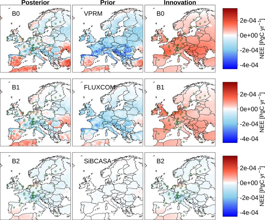
7876                                                                S. Munassar et al.: NEE estimates 2006–2019 over Europe

1   Introduction                                                     cies in simulating the atmospheric transport. The structure
                                                                     of prior uncertainty (e.g. uncertainties in the prior biosphere
The atmospheric mole fractions of greenhouse gases (GHGs)            flux estimates) is of particular importance as it determines
like CO2 , CH4 , and N2 O have drastically increased since           the way in which the flux corrections calculated from the data
the industrial era began (Friedlingstein et al., 2019), primar-      information should be spread in space and time (Chevallier
ily because of anthropogenic GHG emissions. As a conse-              et al., 2012; Kountouris et al., 2015) Defining proper error
quence, the globally averaged surface air temperature has            covariance matrices in both flux and measurement space is
risen by 0.87 ◦ C from 1850 to 2015 (Jia et al., 2019). Car-         therefore essential to obtain an optimal estimate of the true
bon dioxide is ranked as the most prominent anthropogenic            fluxes. Non-optimised flux components used as prescribed
GHG owing to its atmospheric abundance, resulting from               fluxes in the inverse frameworks should be provided with the
(a) the natural exchange through the biogeochemical interac-         highest achievable confidence, as any uncertainty in these
tions with the organic molecules in the biosphere and hydro-         components will directly modify the estimated biosphere–
sphere (represented by the net primary productivity – NPP),          atmosphere fluxes.
(b) significant anthropogenic emissions from burning of fos-            Here, we present NEE estimates from a pre-operational re-
sil carbon and from cement production, and (c) land use              gional inversion system set-up over Europe covering 14 years
changes such as deforestation. The largest uptake of atmo-           since 2006. An ensemble is created by varying (a) a priori
spheric CO2 is carried out through terrestrial gross primary         biogenic fluxes, (b) a priori ocean fluxes, and (c) the number
production (GPP) and thought to derive an uptake of about            of available atmospheric observation sites in order to esti-
one-third of anthropogenic emissions owing to the enhance-           mate their impact on a posteriori optimised biogenic fluxes.
ment of photosynthetic CO2 uptake in the recent decades              We furthermore discuss the interannual variability (IAV) over
(Cai and Prentice, 2020). However, measurements of NEE               this period, with a special focus on the changes in NEE in
(net ecosystem exchange) cannot be easily achieved at finer          2018 and 2019, specifically in light of the water availabil-
spatial and temporal scales over the globe. Ancillary data           ity and temperature variations that occurred in the wake of
from the atmosphere and the biosphere are thus applied in the        anomalously warm and dry conditions over the continent.
inverse modelling set-ups to estimate the natural CO2 fluxes.        These changes are analysed using the seasonal and annual
Such a method of using atmospheric data to constrain NEE             NEE fluxes aggregated over different subregions in Europe.
obtained from the terrestrial biogenic models is also called a          The inversion set-up, observational dataset, and prior
top–down method.                                                     fluxes used are described in Sect. 2, including details on en-
   The continuous expansion of GHG in situ measurement               semble member configuration. A statistical analysis of uncer-
capabilities enabled atmospheric tracer inversion systems to         tainty and spreads over the ensembles of inversions is pre-
better infer the sources and sinks of CO2 at global (Ciais et        sented and discussed in Sect. 3.1. Section 3.2 presents the
al., 2010; Enting et al., 1995; Kaminski et al., 1999; Röden-        NEE estimated in the pre-operational inverse system based
beck et al., 2003) and regional scales (Gerbig et al., 2003;         on several analysed cases. Finally, discussions and conclu-
Kountouris et al., 2018b; Lauvaux et al., 2016). Meanwhile,          sions are summarised in Sect. 4.
regional atmospheric inversions have employed atmospheric
transport models at a finer spatial resolution to deal with the
                                                                     2     Methods
complex atmospheric circulation at continental measurement
stations (Broquet et al., 2013; Lauvaux et al., 2016; Monteil        2.1    Inversion framework
et al., 2020).
   The observational site network across Europe has been             The CarboScope Regional inversion system (CSR) is used to
markedly homogenised since the Integrated Carbon Obser-              infer NEE from observed atmospheric CO2 dry mole frac-
vation System (ICOS) was established in 2015, allowing for           tions at a high spatiotemporal resolution over Europe. The
a better estimation of the regional budgets of CO2 over Eu-          CSR makes use of Bayesian inference to regularise the solu-
rope (Monteil et al., 2020). Consequently, this has allowed          tion of the under-determined inverse problem (i.e. there are
for a better understanding of the impacts of climate extremes        more unknown fluxes than atmospheric observations). For
on ecosystem productivity such as the drought episode that           details about the mathematical concepts, we refer the reader
occurred in 2018 (Bastos et al., 2020; Rödenbeck et al., 2020;       to Rödenbeck (2005); the specifications of the set-up largely
Thompson et al., 2020). The inversions typically assume an-          follow previous studies by Kountouris et al. (2018a, b). The
thropogenic emissions to be well known and thus target the           inversion in the regional domain is embedded into the global
more uncertain biosphere–atmosphere fluxes.                          atmosphere using the “two-step scheme” described in Rö-
   The regional inversion framework encounters various               denbeck et al. (2009). The system scheme allows for the use
sources of uncertainties, such as (1) the uncertainty of a priori    of far-field contributions calculated from optimised fluxes
knowledge (necessary in the Bayesian framework inversions            in a separate global inversion run within the regional inver-
to regularise the solution of the ill-posed inverse problem)         sion without a direct nesting between the global and regional
and (2) the representation error resulting from the inaccura-        models at the boundaries in space and time. A global for-

Atmos. Chem. Phys., 22, 7875–7892, 2022                                               https://doi.org/10.5194/acp-22-7875-2022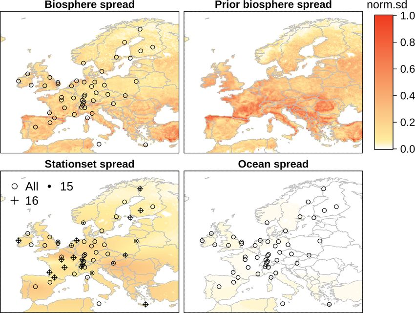
S. Munassar et al.: NEE estimates 2006–2019 over Europe                                                                     7877

ward run is then carried out using “global” observations to        most significant of these changes occurred on 26 June 2013,
obtain simulated concentrations for the regional sites. A sec-     when the vertical resolution of the HRES model was in-
ond forward run is conducted applying zero fluxes outside of       creased from L91 to L137. In our modelling framework that
the regional domain. This can be regarded as a regional run        translates into a 150 % increase in vertical resolution, as we
utilising a global transport model at a coarse spatial resolu-     use 60 and 90 levels (surface to approximately 20.1 km a.g.l.)
tion. For each simulated site, the subtraction of the “regional”   as input data before and after June 2013, respectively. The
signal from that simulated from the global run results in the      upstream influence is simulated over the past 10 d by releas-
far-field contribution at the sites within the regional domain.    ing 100 virtual particles at the sampling heights of stations
Subtracting the latter from the measurements yields the re-        (receptors). Additionally, we use the Eulerian global model
maining regional mixing ratio that is used in the regional in-     TM3 (Heimann and Körner, 2003) within the CarboScope
version, which applies the regional-scale transport model at       global inversion framework (Rödenbeck et al., 2003) to pro-
a finer spatial resolution.                                        vide the far-field contributions to the regional domain at a
   The inversion searches for the optimal flux vector at 3-        coarser spatial resolution of 5◦ (longitude) × 4◦ (latitude).
hourly temporal resolution through minimising the cost func-
tion J (Eq. 1) with respect to the adjustable parameters p         2.2   Atmospheric data
(indicated in Eq. 2) that are assumed to have zero mean and
unit variance:                                                     Since CO2 dry mole fractions are the main constraint of the
                                                                   inversion system, we have aimed in our study to maximise
           1 T
J = Jc +     p p.                                           (1)    the data coverage by using the observations available through
           2                                                       the ICOS network as well as further atmospheric observa-
In CSR, the a priori probability distribution of the fluxes is     tion sites (both ICOS-associated and independent). All of the
defined in a different way than the traditional way through a      datasets are high-quality products of the level-2 ICOS At-
linear flux model f . This flux model is written as a function     mospheric Release, which underwent a strict filtration pro-
of a fixed term f fix and an adjustable term containing the in-    cedure described in Hazan et al. (2016). This homogenised
formation of flux uncertainties and correlations in the matrix     data treatment makes the data suitable for inverse modelling.
F, in which the covariance matrix is implicitly defined:           For measurement sites with multiple sampling levels, the top
                                                                   one is chosen, as this one is expected to be represented best
f = f fix + F p.                                            (2)    in the STILT transport model.
                                                                      The core of our observational dataset consists of data
J c in Eq. (1) represents the observational constraint term        from 44 sites collected in the ICOS Carbon Portal under
(Eq. 3), consisting of the model–data mismatch (cmeas −cmod )      the 2018 drought initiative (https://doi.org/10.18160/ERE9-
and the respective observation error covariance matrix Qc          9D85, Drought 2018 Team and ICOS Atmosphere Thematic
(also containing the transport and representativeness uncer-       Centre, 2020), covering the period 2006–2018. This base
tainty):                                                           dataset was extended into 2019 by the level-2 data (L2) re-
     1                                                             leased by ICOS in 2020 as well as included data from four
J c = (cmeas − cmod )T Q−1
                        c (cmeas − cmod ).                  (3)    new sites. From the total number of sites, 23 are currently
     2
                                                                   ICOS-labelled and have provided data since 2015, while the
The modelled concentrations cmod are calculated using the          rest are non-labelled sites, providing datasets since 2006.
atmospheric transport model over the measurement values            Figure 1 shows the distribution of all sites throughout the do-
cmeas sampled at different times and locations. For a detailed     main of Europe. The figure also shows the division of the
mathematical description of the inversion scheme, the reader       domain into six subregions (Northern, Southern, Western,
is referred to Rödenbeck (2005).                                   Eastern, South-eastern, and Central Europe) used for post-
   Atmospheric transport is simulated by the Stochastic            processing, to outline the impact of the observational con-
Time-Inverted Lagrangian Transport (STILT) model (Lin et           straint distribution on posterior fluxes.
al., 2003), which is utilised to calculate surface influences         The representation error is assumed to be specific for dif-
at the stations (i.e. “footprints”) at a spatial resolution of     ferent station types, which are categorised as five classes ac-
0.25◦ (longitude) × 0.25◦ (latitude) over hourly time inter-       cording to the ability for regional transport models to reason-
vals. The model is driven by meteorological fields from the        ably simulate the atmospheric concentration, given the vari-
high-resolution implementation of the Integrated Forecast-         able complexity of representing the local circulation, over
ing System (IFS HRES) model of the European Centre for             each station (Rödenbeck, 2005). Weekly representation er-
Medium Range Weather Forecasts (ECMWF), extracted at               rors are presented in Table 1, defining the measurement er-
a 0.25◦ × 0.25◦ horizontal and 3-hourly temporal resolution.       ror covariance matrix in the cost function. The observations
The overall quality of the driving meteorological fields in-       are mostly provided at an hourly frequency, especially in re-
creased following the evolution of the forecast system, which      cent years. We also include measurements from flask sam-
underwent regular updates throughout the study period. The         pling (mostly weekly) when available from the correspond-

https://doi.org/10.5194/acp-22-7875-2022                                          Atmos. Chem. Phys., 22, 7875–7892, 2022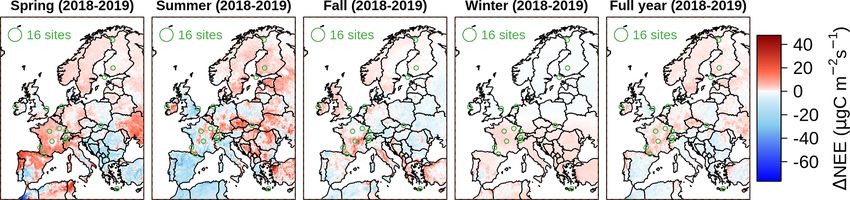
7878                                                                 S. Munassar et al.: NEE estimates 2006–2019 over Europe

                                                                      sphere models at an hourly temporal resolution. Three bio-
                                                                      sphere models were used as priors in the inversion runs.
                                                                      The first is the Vegetation Photosynthesis and Respiration
                                                                      Model, VPRM (Mahadevan et al., 2008). VPRM is a di-
                                                                      agnostic model driven by shortwave radiation and temper-
                                                                      ature at 2 m from the ECMWF’s high-resolution operational
                                                                      forecast product (IFS HRES). To calculate NEE and respi-
                                                                      ration fluxes, it uses MODIS (Moderate Resolution Imaging
                                                                      Spectroradiometer) indices derived from surface reflectance,
                                                                      namely the Enhanced Vegetation Index (EVI) and land sur-
                                                                      face water index (LSWI) together with type-specific veg-
                                                                      etation parameters optimised against the eddy covariance
                                                                      (EC) data. Parameter values for VPRM previously used by
                                                                      Kountouris et al. (2018b) were updated using the most re-
                                                                      cent EC data and are available at https://www.bgc-jena.mpg.
                                                                      de/bsi/index.php/Services/VPRMparam (last access: 20 Oc-
                                                                      tober 2021). The second biosphere prior is from the data-
Figure 1. Station network distribution over Europe. Differ-
                                                                      driven modelling approach FLUXCOM, which combines
ent graphical symbols denote the type of station classifications;
coloured regions indicate Central Europe (green), Northern Europe     eddy covariance measurements and satellite observations in
(blue), Western Europe (purple), Southern Europe (orange), Eastern    several machine learning algorithms to quantify the surface–
Europe (yellow), and South-eastern Europe (light red).                atmosphere energy and carbon fluxes (Jung et al., 2020).
                                                                      Here, we use an extension of the modelling set-up described
                                                                      in Bodesheim et al. (2018), which employs daily and hourly
ing sites. To better represent the well-mixed boundary layer          surface meteorological information from ERA5 as well as
in the STILT model, we limit our analyses to measurements             a mean annual cycle of satellite data to produce NEE esti-
of 6 h daytime for all stations, i.e. 11:00 to 16:00 LT, except       mates at an hourly temporal and 0.5◦ spatial resolution. It
for mountain sites. For the latter, night-time hours (23:00           should be noted that the magnitude of interannual changes
to 04:00 LT) are chosen, as mountain sites experience free-           in the data-driven flux estimates is generally found to be
tropospheric conditions, depending on the mountain height.            unrealistically small (Jung et al., 2011). The terrestrial bio-
Particularly before establishing ICOS in 2015, the variabil-          sphere model SiBCASA (Schaefer et al., 2008) is used as
ity of station data coverage across the period of interest            the third biosphere model. SiBCASA is a combined frame-
was rather high, underlining the sparsity of available data           work based on the Simple Biosphere (SiB) model and the
(Fig. 2). Since then, the site network over Europe has been           Carnegie–Ames–Stanford Approach (CASA) model. As ex-
markedly expanded as new stations have been installed. It             plained in Schaefer et al. (2008), gross primary productivity
should be noted that the variability in data coverage is ex-          (GPP) is calculated by SiB assuming that it is in balance with
pected to result in an inconsistency of annual flux variations.       heterotrophic and autotrophic respiration (RH , RA ), mean-
Therefore, we combined stations into three subsets: (a) the           ing that diurnal and seasonal variations are well represented;
full set of stations, referred to as “all sites”, (b) a subset        however, the long-term terrestrial carbon changes cannot be
of 15 stations that have consistent coverage from 2006 to             predicted by SiB component alone. CASA fills this gap as it
2019, to which we will refer as “core sites”, and (c) a third         includes a light-use-efficiency model to estimate net primary
subset of 16 stations that do not have gaps longer than 1             productivity (NPP, equal to GPP – RA ). In turn, CASA can-
month during 2015–2019, subsequently referred to as “re-              not calculate NEE during night-time. Therefore, combining
cent sites”. The far-field contributions provided to the re-          both models in a hybrid version of SiBCASA combines the
gional domain were calculated in the two-step inversion ap-           advantages in their biophysical and biogeochemical aspects
proach (Rödenbeck et al., 2009) using a global observational          to calculate NEE from RH , RA (SiB), and NPP (CASA).
record from 75 sites (https://doi.org/10.17871/CarboScope-               Following Kountouris et al. (2018b), we assume that the
s10oc_v2020, Rödenbeck, 2020), which has the best data                spatial correlation of the prior uncertainty follows a hyper-
coverage in the 2010–2019 period.                                     bolic decay function, similar to the inversion case nBVH (no
                                                                      Bias VPRM as prior with a hyperbolic decaying correlation
2.3    A priori fluxes
                                                                      of the spatial uncertainty structure) described in that study.
                                                                      In this case, the annually aggregated uncertainty matches the
Terrestrial ecosystem flux models are utilised to provide prior       assumed prior uncertainty without the need for an additional
knowledge of biogenic fluxes (NEE, defined as net ecosys-             bias term in the biosphere flux model. The spatial correlation
tem exchange). To appropriately represent the diurnal cycle           length scales are 66.4 km in the zonal direction and 33.2 km
in our modelling framework, NEE is obtained from the bio-             in the meridional direction. One notable difference in the cur-

Atmos. Chem. Phys., 22, 7875–7892, 2022                                                https://doi.org/10.5194/acp-22-7875-2022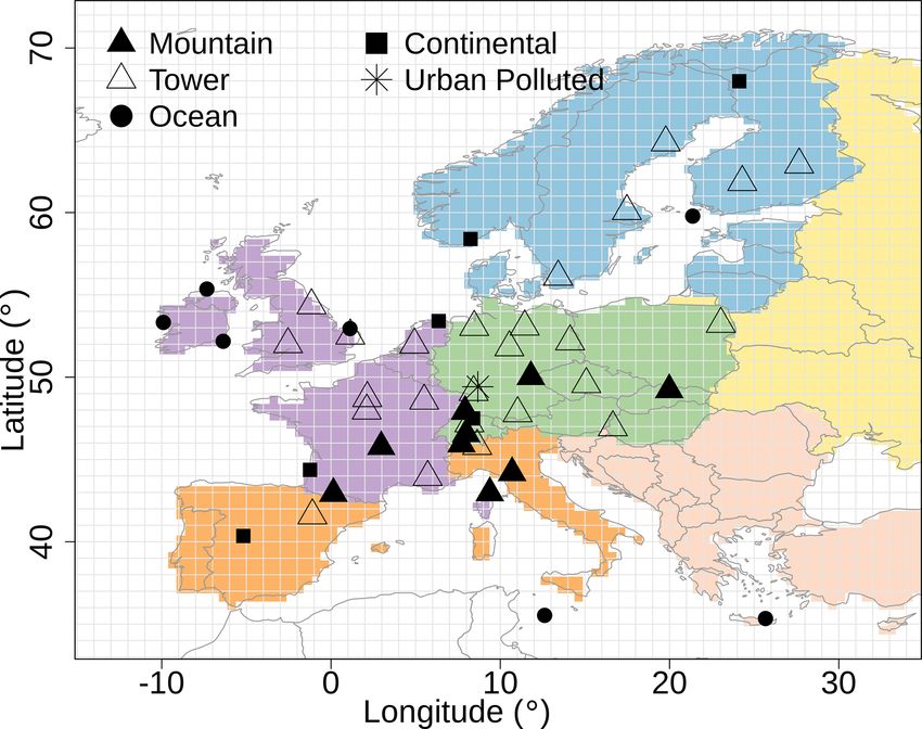
S. Munassar et al.: NEE estimates 2006–2019 over Europe                                                                           7879

Table 1. Representation error of station locations.

                                Classification          Mountain     Tower     Ocean    Continental   Urban
                                Code                    M            T         S        C             UP
                                Error (µmol mol−1 )     1.5          1.5       1.5      2.5           4

Figure 2. Dataset density measured from 2006 until 2019 over Europe. Yellow to red colour scale denotes monthly-averaged dry mole
fractions of CO2 . Symbols on the right-hand axis: C – core site; R – recent site.

rent work is the improved implementation of the directional                specific emission inventories of EDGAR-v4.3 (Emissions
dependence, with a twofold increase in decay distance in the               Database for Global Atmospheric Research), and further pro-
meridional direction. Temporarily, prior uncertainties are as-             cessed following the COFFEE approach (Steinbach et al.,
sumed to be correlated over 30 d, as found in Kountouris et                2011) to include diurnal, weekly , seasonal, and annual vari-
al. (2015).                                                                ations. These emissions are updated annually according to
   Ocean CO2 fluxes and anthropogenic emissions are re-                    national consumption data from the BP (British Petroleum)
garded as prescribed fluxes in the inversion system. Ocean                 statistical review of world energy (BP Annual Report 2019)
fluxes are taken from two sources at a coarse spatial reso-                and are available from the ICOS Carbon Portal under
lution, (5 × 4◦ ): a climatological flux product with monthly              https://doi.org/10.18160/Y9QV-S113 (Karstens, 2019). We
fluxes of Fletcher et al. (2007) and the CarboScope pCO2 -                 estimate the uncertainty associated with the anthropogenic
based ocean flux, providing fluxes at 6-hourly temporal res-               emissions for 2014 by comparing fossil fuel emissions over
olution (Rödenbeck et al., 2013). The CarboScope pCO2 -                    the EU27+UK as reported in Petrescu et al. (2021). In their
based ocean fluxes comprise seasonal, interannual, and day-                study, they have reported data from eight sources, including
to-day variations and are updated in the CarboScope global                 an EDGAR product, and the spread over the annual total is
inversion based on the Surface Ocean CO2 Atlas pCO2 ob-                    0.038 PgC with a mean of 0.974 PgC yr−1 , suggesting un-
servations (SOCAT). We have used fossil fuel emissions                     certainty of around 4 % among those emission products. If
developed in-house based on the category and fuel-type-                    we assume this is also the uncertainty of our anthropogenic

https://doi.org/10.5194/acp-22-7875-2022                                                  Atmos. Chem. Phys., 22, 7875–7892, 2022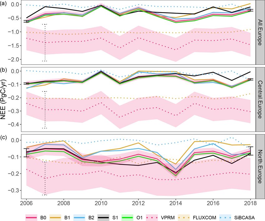
7880                                                               S. Munassar et al.: NEE estimates 2006–2019 over Europe

emission product, we can compare it to the spread of prior             It is noteworthy that there is a striking similarity in inter-
NEE in our study (0.940 PgC yr−1 ). As a result, prescrib-          annual variations between the a posteriori fluxes and both
ing fossil fuel in the inversion and solving for NEE is ap-         VPRM and SiBCASA prior fluxes for the years 2009–2013.
propriate; however, when interpreting posterior biosphere–          This agreement does not necessarily mean that posterior in-
atmosphere exchange fluxes, one has to take into account that       terannual variability (IAV) is driven by biosphere models.
part of the fluxes and their variability might be compensating      This can be deduced from B1 (FLUXCOM) estimates from
for errors in anthropogenic emissions.                              which the IAV differs in both the prior and posterior fluxes
                                                                    and where FLUXCOM NEE has weak interannual variations.
2.4    Set-up of the inversion runs                                 Instead, VPRM and SiBCASA are likely to import this sig-
                                                                    nal from the meteorological data used to force these models.
We conduct three ensembles of inversion runs listed in Ta-          However, the VPRM model overestimates the mean CO2 up-
ble 2 utilising different set-ups of prior products (biosphere      take compared to the a posteriori fluxes, while SiBCASA un-
and ocean ensembles) as well as selected sets of observa-           derestimates the mean CO2 uptake, and this dissimilarity is
tional data (station set ensemble). The inversion runs are la-      persistent for all years as well.
belled with unique codes for reference. B0 is defined as the           The statistical uncertainty and spreads over the ensembles
base case of our analysis. It is configured using default set-      are evaluated and affect our data (Fig. 3). It is noticed that the
tings of the inversion runs, with biogenic fluxes from VPRM         spreads over the posterior fluxes and prior fluxes are compa-
and climatological ocean fluxes, and using all available atmo-      rable with the corresponding uncertainties over the full do-
spheric data as input. In the biosphere ensemble (consisting        main (All Europe), Central Europe, and Northern Europe.
of B0, B1, and B2), FLUXCOM and SiBCASA replace the                 Note that calculating the spread over a small size of sam-
VPRM model in both B1 and B2, respectively, allowing for            ples might not reflect the true standard deviation. There is a
a distinction between the effect of using different prior flux      clear reduction in uncertainty and spread in posterior fluxes
models on posterior NEE. This ensemble of inversions was            either over the full domain (All Europe) or in subregions like
performed for the period 2006–2018, as the availability of          Central and Northern Europe. Unlike prior uncertainty, pos-
SiBCASA fluxes was limited to this period of time. In the           terior uncertainty slightly differs from year to year following
ocean ensemble, we replace the climatological ocean fluxes          the number of atmospheric sites available (Fig. 2). This gets
used in B0 with the pCO2 -based CarboScope ocean fluxes in          even clearer when looking at the marked reduction in the pos-
O1. The station set ensemble is formed by running the inver-        terior uncertainty in Central Europe as well as in regions with
sion with varying measurement station subsets as explained          high station density, resulting in a stronger observational con-
in Sect. 2.2: B0 – all sites; S1 – core sites; and S2 – recent      straint. In contrast to Central Europe, a smaller reduction in
sites. For each of the three ensembles of inversions, its spread    posterior spread is found in Northern Europe as well as in
is calculated as the standard deviation of the differences be-      other regions where there are few or no stations (e.g. Eastern
tween each ensemble member and the ensemble mean over               Europe, Fig. S1 in the Supplement). In this case, NEE esti-
the respective overlapping period of time. The statistical un-      mates are not well constrained by atmospheric data. Instead,
certainty is calculated in the inverse system based on model–       a posteriori flux is driven by the inversion using biosphere
data mismatch and the prescribed prior uncertainty and was          models and their uncertainty, particularly for the distant ar-
performed for the base case inversion (B0) as it remains iden-      eas that cannot be constrained by observations through the
tical independent of the biosphere model used.                      spatial correlation. Table 3 denotes the reduction in the bio-
                                                                    sphere ensemble spread in the a posteriori spread relative to
3     Results                                                       the a priori spread over the full domain, Central and North-
                                                                    ern Europe (95.1 %, 96.0 %, and 74.8 %, respectively). It in-
3.1    Statistical analysis of ensemble uncertainties               dicates less reduction in Northern Europe due to the sparse-
                                                                    ness of observational sites. The large reduction in spread in
The annual NEE estimates among the biosphere ensemble
                                                                    Central Europe reflects a notable dependency of NEE esti-
(Fig. 3) show good agreement across the three biosphere
                                                                    mates on the atmospheric measurements, substantially where
models but also across S1 and O1 inversions, yielding similar
                                                                    the observation network is dense.
budgets of CO2 fluxes over the full domain. The findings sug-
                                                                       To analyse the seasonal variations, the seasonal cycle from
gest that atmospheric data constraints are more dominated in
                                                                    B0, B1, B2, S1, and O1 inversions is averaged over 13 years
the posterior NEE fluxes in comparison with the prior con-
                                                                    for the full domain of Europe together with the correspond-
straint. Subregions that are characterised by strong observa-
                                                                    ing biogenic prior fluxes for VPRM, FLUXCOM, and SiB-
tional constraints such as Central Europe show a closer con-
                                                                    CASA (Fig. 4). Results show good agreement amid a pos-
sistency in the posterior fluxes despite large prior differences
                                                                    teriori results of all inversions, while prior biosphere mod-
among the biosphere models compared to the regions less
                                                                    els show large differences, a pattern similar to the one seen
constrained by atmospheric data, such as Northern Europe.
                                                                    over the annual fluxes in Fig. 3. Nevertheless, posterior NEE
                                                                    fluxes estimated in the S1 inversion show differences dur-

Atmos. Chem. Phys., 22, 7875–7892, 2022                                               https://doi.org/10.5194/acp-22-7875-2022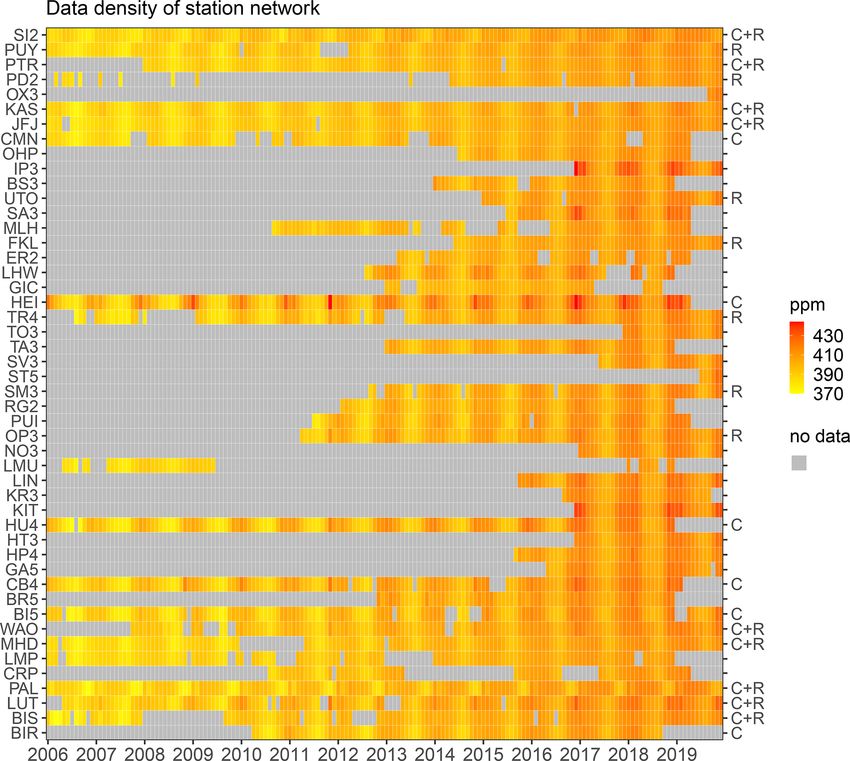
S. Munassar et al.: NEE estimates 2006–2019 over Europe                                                                                  7881

Table 2. Set-ups of the inversions.

                                      Inv. code   Biosphere     Ocean           Station set     Time period
                                      B0 (base)   VPRM          Mikaloff        all             2006–2018
                                      B1          FLUXCOM       Mikaloff        all             2006–2018
                                      B2          SiBCASA       Mikaloff        all             2006–2018
                                      O1          VPRM          CarboScope      all             2006–2018
                                      S1          VPRM          Mikaloff        core sites      2006–2019
                                      S2          VPRM          Mikaloff        recent sites    2015–2019

Figure 3. NEE fluxes estimated using B0, B1, B2, S1, and O1 inversions for the 2006–2018 period over the full domain of Europe (a),
Central Europe (b), and Northern Europe (c). Posterior fluxes are plotted with solid lines and their a priori fluxes as the dotted lines. Priors
and posteriors of the biogenic ensemble are distinguished by identical colours for each modelled scenario. Light red shadowing denotes the
statistical uncertainty and error bars indicate the spread among the biosphere inversions’ ensemble.

ing May–August when compared with the estimates of other                  ble spread over the a priori biosphere models agrees with the
runs, reflecting a larger sensitivity of IAV to summer fluxes             assumed prior uncertainty, with a relatively high value (about
when applying a different set of stations. In addition, the dif-          0.44 PgC yr−1 domain-wide) indicating large discrepancies
ference in posterior fluxes seen in Fig. 3 over the annually ag-          between prior flux models. This confirms that the prior un-
gregated estimates computed from the B1 inversion over the                certainty assumed in the CSR system is realistic. The IAV
period 2014–2018 largely results from the estimates during                of B0 was calculated separately for prior and posterior fluxes
May and June when comparing them to the rest of biosphere                 (blue bars) from the anomalies relative to the long-term mean
ensemble elements (Fig. 4).                                               to reveal the magnitudes of interannual deviation in compar-
   Figure 5 illustrates the statistical uncertainty and the               ison with the spread variability.
spread through the overall ensembles of inversions (listed                   In terms of the spread of the biosphere ensemble, the stan-
in Table 2) calculated annually over three regions. As was                dard deviation of posterior fluxes declines from 0.666 to
discussed in the time series of NEE (Fig. 3), a reduction in              0.032 PgC yr−1 over All Europe. Spatial differences are ex-
posterior NEE uncertainty with respect to the assumed prior               pected as stations are not evenly distributed across the do-
uncertainty is clear (dark grey bars in Fig. 5). A larger reduc-          main of Europe. This can be noticed from the spread over
tion is realised in Central Europe, emphasising a strong atmo-            Central Europe (a large number of stations, 18 sites) and
spheric signal constraint in the inversion. The spread among              Northern Europe (a smaller number of stations, 8 sites). As
ensemble members (Fig. 5, yellow bars) represents the stan-               a result, the lack of observations leads to inflating the spread
dard deviation of the respective inversion results. The ensem-            over the biosphere ensembles.

https://doi.org/10.5194/acp-22-7875-2022                                                      Atmos. Chem. Phys., 22, 7875–7892, 2022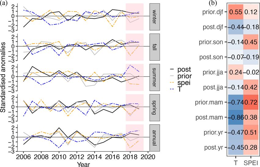
7882                                                                      S. Munassar et al.: NEE estimates 2006–2019 over Europe

Table 3. Reduction in the biosphere ensemble NEE spread over Europe.

                                   Region               Prior spread     Posterior spread   Spread reduction
                                                         (PgC yr−1 )          (PgC yr−1 )               (%)
                                   All Europe                  0.666               0.032               95.1
                                   Central Europe              0.137               0.005               96.0
                                   Northern Europe             0.098               0.024               74.8
                                   Southern Europe             0.061               0.023               61.7
                                   Eastern Europe              0.129               0.024               80.9
                                   Western Europe              0.142               0.015               89.1

Figure 4. Seasonal cycle of NEE calculated as the average of monthly fluxes over 13 years estimated using the ensembles of inversions
(solid lines) B0, B1, B2, S1, and O1 as well as the biogenic prior fluxes (dotted lines) obtained from VPRM, FLUXCOM, and SiBCASA.

                                                                            assess the posterior uncertainty. In addition, NEE estimated
                                                                            among the station set ensemble suggests that while in all
                                                                            cases the posterior fluxes are data-driven, modification of the
                                                                            observation inputs leads to interannual variations. The spread
                                                                            of the ocean ensemble remains the smallest in all the regions,
                                                                            indicating quite a weak dependency of posterior NEE esti-
                                                                            mates on ocean fluxes, in particular over inland regions (e.g.
                                                                            Central Europe).
                                                                               The spatially distributed spread of all ensembles is de-
                                                                            picted in Fig. 6. In this instance, the standard deviation was
Figure 5. Spread uncertainties calculated from three inversion en-          calculated for each grid cell rather than aggregating fluxes
sembles of biosphere, ocean, and station set (yellow bars). Grey bars       over regions first and then computing the spread (Fig. 5).
refer to the statistical uncertainties, and blue bars denote the stan-      The spatial spread here illustrates the deviations in the bio-
dard deviations of IAV.                                                     sphere ensemble (“Biosphere spread”), the biosphere models
                                                                            (“Prior biosphere spread”), the station set ensemble (“Sta-
                                                                            tionset spread”), and the ocean ensemble (“Ocean spread”).
   The largest impact on NEE estimates in the ensembles is                  The maximum spread of 0.191 × 10⁻⁴ (PgC yr−1 ) was ob-
observed when the spread over the station set ensemble is                   served over the a priori terrestrial biosphere models, par-
analysed. In this regard, a robust analysis can be based on a               ticularly concentrated in Central and Southern Europe. The
subset from Central Europe, as the subsets of stations in this              spread of the a posteriori biosphere ensemble is signifi-
region clearly contrast in the two ensemble members (core                   cantly reduced. In the station set ensemble, isolated stations
sites and recent sites). The spread of the station set ensem-               like Hegyhátsál in Hungary and Sierra de Gredos in Spain
ble was found to be 0.11 PgC yr−1 – larger than those re-                   demonstrate a relatively high impact on the NEE spatial pat-
sulting from the biosphere and ocean ensembles (0.05 and                    terns over broader areas, reflecting the inversion correlation
0.02 PgC yr−1 , respectively). It is noteworthy that the spread             length. However, such an impact is not clearly realised in the
in the station set ensemble is slightly larger than the statistical         Stationset spread map amid dense clusters of sites due to the
uncertainty, highlighting the importance of performing en-                  commutative constraint that compensates for the excluded
sembles of inversions using different numbers of stations to

Atmos. Chem. Phys., 22, 7875–7892, 2022                                                       https://doi.org/10.5194/acp-22-7875-2022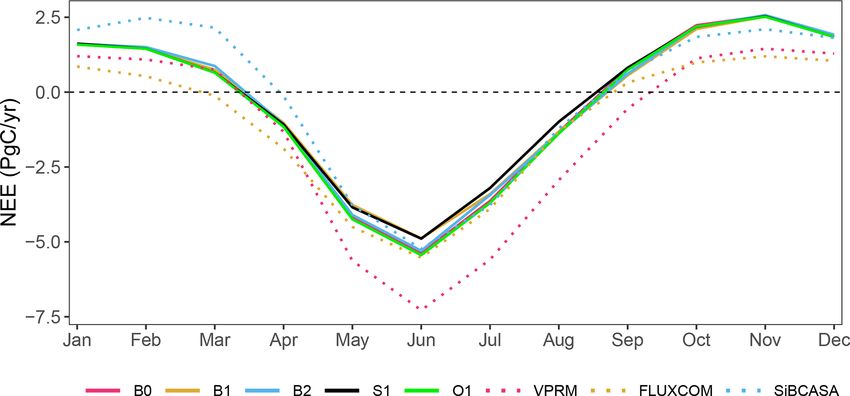
S. Munassar et al.: NEE estimates 2006–2019 over Europe                                                                       7883

sites within the subsets of stations. These results highlight       ble with findings of NEE anomalies reported by Rödenbeck
the importance of defining a proper function of spatial corre-      et al. (2020) but estimated using different global inversion
lation decay in the prior uncertainty structure. Quite a small      runs (2019 was not included in that study). Herein, we shed
influence is seen through the spread over the ocean, where          more light on 2019 NEE estimates which suggest an even
a slight impact emerges only in wider coastal regions, being        weaker uptake of CO2 in comparison with the summer of
almost negligible inland (e.g. in Central and Eastern Europe).      2018. It is noticed that the posterior fluxes estimated using
   Figure 7 indicates the spatial distributions of prior and pos-   the biosphere model FLUXCOM exhibit the largest anomaly
terior NEE averaged over the full 13-year period, estimated         of NEE during the summer of 2019. Despite slight differ-
from B0, B1, and B2 inversions as well as the correspond-           ences in the amplitude of IAV, there is good agreement in
ing innovation of fluxes (the difference between posterior and      the posterior fluxes estimated with both the FLUXCOM and
prior fluxes). Positive corrections have been made to the bio-      VPRM models. Such common agreement is inherited from
sphere flux models that are regarded to be negatively biased        the identical observations used in both the inversion runs,
(VPRM and FLUXCOM, as was unequivocally confirmed                   as demonstrated in the case of the biosphere ensemble in
by the annual time series of NEE in Fig. 3). In contrast,           Sect. 3.1. Therefore, the IAV in this case is more likely to be
SiBCASA results are closer to the mean of posterior fluxes,         attributed to climate anomalies, in particular during drought
with a small domain-wide negative correction, except for lo-        occurrence in the growing season.
cal positive innovations seen over Northern Germany and the            The agreement between posterior fluxes using FLUXCOM
Western Mediterranean coast.                                        and prior fluxes of VPRM in the spring season confirms two
                                                                    important conjectures: (1) posterior IAV are largely derived
3.2   NEE estimates of 2018 and 2019 in a
                                                                    by atmospheric data regardless of the biosphere model used;
      pre-operational system
                                                                    (2) the VPRM model can capture year-to-year variations dur-
                                                                    ing spring, reflecting its capability to represent dynamic bio-
In this section, we present CO2 fluxes for 2 selected years         spheric activity during the growing season. It is clear that
estimated in a pre-operational system in the context of long-       FLUXCOM exhibits remarkably weaker annual variations
term estimates. In synergy with the research project VERIFY         during spring and fall in comparison with the VPRM and
in alignment with the scope of the Paris Climate Agreement,         the a posteriori fluxes. In winter, the VPRM model agrees
the system is used to provide annual updates of estimated           well with FLUXCOM in the interannual variations, showing
fluxes over Europe once the atmospheric observations and            less IAV compared to the NEE estimates. We attribute this to
auxiliary data required to force prior flux models and atmo-        the lower signal of temperature assimilated in the biosphere
spheric transport models are available. The CSR is described        models from the meteorological data as well as less infor-
as a “pre-operational system”, as it is still under develop-        mation of radiation reflectance obtained from the remote-
ment from year to year. The period of interest is chosen to         sensing data due to dominant cloudy scenes in winter, pro-
start from 2006, in which a better coverage of observations         vided that the VPRM and FLUXCOM models use forcing
exists within the domain of Europe. Here, we give special           data from meteorology and remote sensing. In addition, mis-
attention to analysis of the drivers of spatiotemporal differ-      representation in the anthropogenic emissions prescribed in
ences in line with climate disturbances that occurred in 2018       the inversion may contribute to the posterior IAV, in particu-
and 2019, during which inaccuracies of estimating the con-          lar during winter due to the fact that the biosphere signal is
tinental fluxes of CO2 have been reported (Friedlingstein et        generally weak.
al., 2019). This is due to the sensitivity of ecosystem respira-       To assess the temporal changes in NEE in response to such
tion and photosynthetic fluxes to extreme events like lasting       climate variations, we compare the seasonal anomalies of
droughts. The analysis here is based on two inversion runs          NEE (prior and posterior) to the anomalies of 2 m air tem-
using observational data only from the subset of core sites         perature and Standardised Precipitation–Evapotranspiration
that have consistent measurements, i.e. (1) the S1 inversion        Index (SPEI) (Beguería et al., 2014) during spring, summer,
set-up and (2) a similar set-up to S1 performed with FLUX-          fall, and winter as well as the annual mean (Fig. 9). Here
COM instead of VPRM. The choice of using consistent mea-            we show estimated NEE integrated over the full domain.
surements is essential to study the IAV to diminish the uncer-      Monthly near-real-time data of SPEI (SPEI01) are obtained
tainty caused by gaps of data coverage over years. The IAV          from https://spei.csic.es/map/maps.html (last access: 24 De-
of estimated CO2 fluxes is then compared with the IAV of            cember 2020) at 1◦ spatial resolution and monthly 2 m air
the biosphere flux models (VPRM and FLUXCOM) used as                temperature accessed via https://psl.noaa.gov/data/gridded/
priors in the two inversion runs.                                   index.html (last access: 11 February 2021) at 0.5◦ spatial
   Summer NEE anomalies between 2006 and 2019 (1NEE,                resolution. The anomalies were normalised with the stan-
Fig. 8) are positive in the years 2007, 2010, 2016, 2018,           dard deviation of the interannual variations since 2006. In
and 2019 indicating that the mean uptake of CO2 during the          addition, Pearson correlation coefficients between posterior
growing season was lower than average in these years. The           fluxes, prior fluxes, temperature, and SPEI for the full year
magnitudes of anomalies during these years are compara-             and calendar seasons were calculated. It is of note that, due to

https://doi.org/10.5194/acp-22-7875-2022                                            Atmos. Chem. Phys., 22, 7875–7892, 2022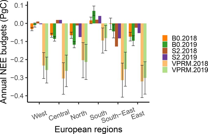
7884                                                                   S. Munassar et al.: NEE estimates 2006–2019 over Europe

Figure 6. Spatial spread of biosphere, prior, station set, and ocean ensembles. Standard deviation (SD) in the legend is normalised over
maximum spread 1.91 × 10⁻⁴ in units of PgC yr−1 per grid pixel. Stations used in the station set ensemble are referred to by circles (B0),
dots (S1), and the plus symbol (S2).

Figure 7. Posterior, prior, and innovation of fluxes (posterior – prior) averaged over the 2006–2018 period calculated from the biosphere
ensemble of inversions (B0, B1, and B2). Green circles refer to observing sites.

Atmos. Chem. Phys., 22, 7875–7892, 2022                                                   https://doi.org/10.5194/acp-22-7875-2022
S. Munassar et al.: NEE estimates 2006–2019 over Europe                                                                              7885

                                                                          alised from the SPEI and temperature anomalies, there is a
                                                                          relatively moderate correlation between estimated NEE and
                                                                          SPEI and temperature at the annual scale over the full domain
                                                                          (Fig. 9b). However, the correlation coefficients vary greatly
                                                                          between seasons. A high anticorrelation (−0.86) between es-
                                                                          timated NEE and temperature is found to be consistent dur-
                                                                          ing spring. In contrast, anticorrelation drastically decreases
                                                                          and turns out to almost vanish in summer and fall. Nonethe-
                                                                          less, the relatively moderate correlation of SPEI with poste-
                                                                          rior NEE during summer is adequate to deduce the lack of
                                                                          SWC under dry conditions through the anticorrelation be-
                                                                          tween SPEI and temperature. This implies that warm con-
                                                                          ditions accelerate the depletion of soil moisture content, in
                                                                          particular in the soil top layer that lacks water content in its
Figure 8. Anomalies of NEE fluxes during spring, summer, fall,            deeper layers to compensate for the higher evaporation rate at
and winter estimated from two inversion runs differing in biosphere       the surface layer. This affects photosynthesis efficiency dur-
models (FLUXCOM in red colour and VPRM in blue colour) using              ing the growing season by decreasing the gross primary pro-
the atmospheric data of core sites. Solid lines indicate the a posteri-   ductivity but also increases the contribution of soil respira-
ori anomalies, while dashed lines refer to the corresponding a priori     tion, which is more pronounced in 2019.
(biosphere models) anomalies.                                                During winter, water availability does not seem to be a
                                                                          limiting factor of NEE as we notice from low correlations
                                                                          between posterior NEE and SPEI. Instead, temperature neg-
the fact that the biosphere model VPRM utilises temperature               atively correlates with posterior NEE indicating that the in-
from meteorological fields and EVI data from the satellite                crease in temperature coincides with enhanced uptake of
sensor MODIS, it is anticipated to systematically correlate               CO2 where photosynthesis can occur, e.g. in evergreen ar-
with temperature and SPEI. Consequently, we mostly devote                 eas. But cold years have more and longer snow cover which
our comparison to the posterior fluxes.                                   decreases photosynthesis, whereas soil heterotrophic respira-
   The findings of standardised anomalies in Fig. 9a show                 tion contributes more to CO2 release since soil temperature
that the decrease in CO2 uptake in 2018 and 2019 during the               is expected to be larger than air temperature owing to snow
growing season was concurrent with a profound deficit of soil             cover insulation. Meanwhile, the anticorrelations between
water content (SWC) (negative SPEI anomalies, dry condi-                  estimated NEE and temperature may result from a misattri-
tions). The reduction or very low SWC also coincided with                 bution of anthropogenic emissions, as warmer winters mean
an unprecedented rise in temperature (positive T anomalies,               less anthropogenic emissions (the opposite holds true for
highest in 2018) across Europe. Being an indicative factor                colder winters). It is of note that X December, X +1 January,
of drought occurrences, SPEI links water availability in the              and X + 1 February are incorporated into the winter estimate
surface including soil moisture (crucial limitation of GPP, es-           of a specific year (X). Figure 10 illustrates the seasonal con-
pecially in the temperate regions) and temperature to the pre-            tribution of NEE to IAV, which is dominated by summer and
cipitation and evapotranspiration rate. Hence, there is quite             spring variability in comparison with winter. We note that the
good agreement between posterior NEE and SPEI not only                    posterior fluxes are in agreement with the biosphere model
at spatial scales but also at temporal scales. The standard de-           VPRM in summer and fall, while the variability of posterior
viations of the interannual variations in posterior NEE, SPEI,            fluxes is larger during winter and smaller during spring com-
and temperature over All Europe in the annual mean through                pared to prior fluxes; the opposite holds true for the prior
the 14 years were equal to 0.17 PgC yr−1 , 0.12, and 0.45 K,              fluxes. Temperature is, however, shown to vary greatly dur-
respectively. When relating the changes occurring during                  ing winter, while the SPEI contribution does not show a sig-
2018 and 2019 to the context of the previous 12 years, the                nificant variability between seasons.
annual anomalies of SPEI were found to decline to more than
twice as much as the climatological deviation: around −0.29               3.2.1   Spatial differences in NEE estimates in 2018 and
in 2018 and to around −0.08 in 2019. As a consequence, pos-                       2019
terior NEE anomalies increased to 0.14 and 0.08 PgC yr−1
above the climatological mean in 2018 and 2019, respec-                   Using an identical set of observation sites for the last 5 years,
tively.                                                                   the S2 inversion demonstrates the differences between NEE
   The excess of annually averaged temperature was predom-                estimates in 2018 and 2019 as seen in Fig. 11. Results em-
inant in 2018 and 2019, reaching around 0.40 and 0.47 ◦ C                 phasise the aftermath of drought episodes, showing a smaller
above the climatological mean, respectively. Despite the fact             uptake of CO2 in France, Germany, and Northern Europe
that the impact of the 2018 and 2019 drought on NEE is re-                during the spring of 2018 (March–April–May), while dur-

https://doi.org/10.5194/acp-22-7875-2022                                                  Atmos. Chem. Phys., 22, 7875–7892, 2022
7886 S. Munassar et al.: NEE estimates 2006–2019 over Europe
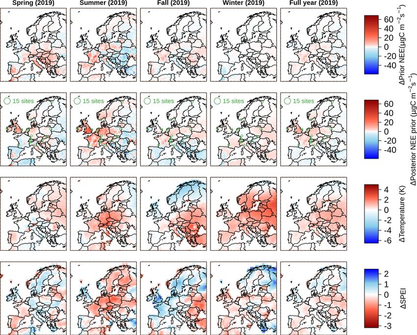
Figure 9. Panel (a) shows the anomalies of posterior NEE (post), prior NEE (prior), SPEI (spei), and 2 m air temperature (T ) standardised
relative to the standard deviation of climatological variations at annual and seasonal scales since 2006 over the full domain of Europe. Units
of NEE and temperature are in PgC yr−1 and K, respectively, while SPEI is unitless. Panel (b) refers to the correlation coefficients of posterior
and prior NEE on the y axis with SPEI and air temperature on the x axis calculated in springs (mam), summers (jja), falls (son), and winters
(djf) and at annual scales (yr) over the full domain of Europe. Note: seasonal T and SPEI correspond to NEE seasons mentioned on the y
axis.
imally small throughout the full domain, while the annual
mean fluxes indicate much smaller uptake in 2018 compared
to 2019. This confirms a longer impact of the drought lasting
from the early growing season during spring until the end
of summer. To explain the changes in spatial distribution of
NEE alongside SPEI and temperature in 2019, anomalies of
NEE were estimated using the S1 inversion with respect to
2006–2018 anomalies. Figure 12 indicates the coincidence of
the large release of CO2 during summer time in Central Eu-
rope with the positive anomalies of temperature and the neg-
ative anomalies of SPEI over those regions. The prior fluxes,
to a lesser extent, show the impact of temperature and SWC
on NEE during the growing season. However, in the United
Kingdom positive NEE anomalies can only be detected from
the posterior fluxes. The positive anomalies of temperature
during winter show a slight impact on NEE (positive anoma-
lies). This can be interpreted as an increase in soil respiration.
The annual budgets of NEE in 2019 and 2018 are sum-
Figure 10. Seasonal contribution to IAV calculated relative to marised in Fig. 13 for six subregions estimated using the B0
14 years for posterior NEE fluxes (post), VPRM NEE fluxes (prior), and S2 inversions. The choice to use the B0 inversion is to
SPEI, and T during the four seasons over the full domain. estimate annual flux budgets of CO2 through assimilating as
many atmospheric observations as possible to strengthen the
observational constraint in the spatial and temporal aspects.
ing the summer of 2019 (June–July–August) the estimates The S2 inversion is specifically used to keep identical obser-
of NEE, to some extent, suggest a higher CO2 release, in vations in 2018 and 2019 for the purpose of assessing the
particular in the United Kingdom, France, Germany, and NEE differences between the 2 years. The annually aggre-
Southern Europe. NEE estimates during the fall of 2018 sug- gated fluxes estimated from the B0 inversion over the full
gest less uptake in Western, Northern, and Southern Europe domain yield −0.28 and −0.22 PgC in 2019 and 2018, re-
compared to the fall of 2019. Obviously, during winter time spectively. The performance of the inversion reflected in the
(December–January–February) the differences are infinites-
Atmos. Chem. Phys., 22, 7875–7892, 2022 https://doi.org/10.5194/acp-22-7875-2022S. Munassar et al.: NEE estimates 2006–2019 over Europe 7887
Figure 11. Differences in NEE estimates for 2018–2019 in seasonal and annual mean calculated from the S2 inversion set-up.
Figure 12. The 2019 anomalies of prior fluxes (first row), posterior NEE estimated from the S1 inversion (second row), 2 m air temperature
(third row), and SPEI (fourth row) relative to 2006–2019 over Europe. Columns denote mean estimates of spring, summer, fall, winter, and
annual NEE estimates, from left to right.
a posteriori fluxes is associated with an uncertainty reduction These results, again, highlight the sensitivity of the inver-
of 85.5 to 88 % with respect to assumed prior uncertainty for sion to data coverage but also the stronger impact of warmer
2019 and 2018, respectively. Likewise, the underlying Euro- summers on NEE, where S2 estimates suggest larger flux
pean regions indicate an uncertainty reduction with different budgets in 2019 compared to 2018 over Western and South-
magnitudes based on atmospheric data availability. The rel- ern Europe. Overall, B0 and S2 results suggest a suppression
atively observationally weak constraint in 2019 has thus re- of GPP, predominantly in Central and Northern Europe.
sulted in a small increment of posterior uncertainty in regions
that have a smaller number of stations. For instance, the un-
certainty in Southern Europe was amplified from 0.018 PgC 4 Discussion and conclusions
in 2018 to 0.027 PgC in 2019, coinciding with an increase in
the net source of CO2 fluxes from 0.016 in 2018 to 0.069 PgC 4.1 Sensitivity of posterior fluxes to input data
in 2019. Despite the data coverage difference in both years,
Southern Europe still shows a larger annual flux of 0.04 PgC The smaller spread in the a posteriori fluxes found through
in 2019 estimated using the S2 inversion in comparison with the ensembles of inversions is evident over All Europe re-
0.02 PgC in 2018. flecting the good performance of the inversion system. In the
biosphere ensemble, flux estimates are not very sensitive to
a priori terrestrial ecosystem fluxes. We deduce this from the
https://doi.org/10.5194/acp-22-7875-2022 Atmos. Chem. Phys., 22, 7875–7892, 20227888 S. Munassar et al.: NEE estimates 2006–2019 over Europe
the results point to a relatively higher influence in the coastal
regions.
Our results denote a comparable reduction in posterior un-
certainty and the spread relative to their a priori (Fig. 5).
It is noteworthy that the indirect effect of statistical poste-
rior uncertainty on the corresponding spread over the ensem-
bles of inversions emerges from the common dependency on
observational data, which predominantly appear in the well-
constrained areas in Germany, France, Benelux, and the UK.
Over such regions, the posterior uncertainty and spreads are
greatly reduced and the inversions tend to converge regard-
less of which prior flux model is used. It is essential to con-
sider the prior uncertainty assumption as well as the prior
error structure in the spatial and temporal aspects. This will
Figure 13. Posterior NEE flux budgets over six European regions determine to which extent the posterior fluxes are dependent
in 2018 and 2019 using the B0 and S2 inversions (dark colours)
on the uncertainty biogenic fluxes, specifically in the regional
compared to their priors from the VPRM model (light colours). Un-
certainties associated with B0 and VPRM fluxes are referred to in
inversions where the degrees of freedom can drastically in-
the error bars. crease following the finer spatial and temporal resolution of
biosphere flux models and atmospheric transport models.
4.2 Response of NEE estimates to climate variation
small spread over the a posteriori fluxes (Fig. 3), occurring
despite major differences in a priori fluxes. Likewise, differ- The linkage between NEE and climate variation has been ex-
ent ocean flux models have the smallest effect on estimating amined via SPEI and temperature as proxy data of climate
NEE, in particular inland, where the ocean–land exchange is variation. The anomalies of SPEI and temperature are anal-
dissipated. However, the spread in the station set ensemble is ysed along with NEE anomalies during the recent years 2018
strongest, at 0.11 PgC yr−1 for the annually aggregated fluxes and 2019 in the context of the period 2006–2017. The recent
over the full domain. This points out a higher sensitivity of drought events decreased the efficiency of GPP, in particu-
the inversion to the number of stations in comparison with lar during spring and summer, where soil moisture markedly
0.06 and 0.02 PgC yr−1 spreads in the biosphere and ocean declined during the summer of 2018 and 2019 accompanied
ensembles, respectively. This effect is most pronounced over with an exceptional rise in temperature (Ma et al., 2020). But
Central Europe, where measurements of CO2 dry mole frac- GPP during spring 2019 showed a higher efficiency (larger
tions are available from a large number of stations, and thus uptake of CO2 ) than the spring of 2018, benefiting from
a contrasting number of sites manifests itself amongst station the increment of temperature, SWC, and light availability.
subsets, given that the station subsets were not selected based The finding is consistent with a study on seasonal NEE over
on geographical locations but on the long record of data cov- North America implemented by Hu et al. (2019) and seems
erage. Further, this finding corroborates the dominant influ- to hold for Northern regions where temperature is substan-
ence of observational constraint on NEE estimates in the bio- tially regarded as a limiting factor to NEE. Additionally,
sphere and ocean ensembles seen through interannual varia- our results showed that Central Europe experienced higher
tions. Such influence is, however, subject to the availability sources of CO2 during 2019, which can be impacted by an
of the atmospheric data which can otherwise be altered by the extended legacy of the drought of 2018, where forests were
prior constraint to maintain the posterior estimates according profoundly stressed and thus their growth was negatively im-
to Bayes’ approach. For example, the relative spread over pacted. MacKay et al. (2012) found an about 17 % reduc-
biosphere ensembles in Northern Europe, having less dense tion in drought plot growth relative to a reference plot and
coverage, increases to 38.4 % compared to 23.9 % in Central showed that growth reduction in the forests across Europe ex-
Europe. Conversely, in the station set ensemble, the spread ceeded this value under drought conditions depending on tree
calculated for Northern Europe was found to be smaller than species. Furthermore, the ecosystem respiration response to
that in Central Europe (51.8 % versus 71.7 %), reflecting the the temperature increment may contribute to such a positive
biogenic flux constraints in this case, given the smaller dif- anomaly, given that temperature anomalies during 2019 over
ferences in observations among the station subsets in this en- Central and Southern Europe were unprecedented, in line
semble. The ocean ensemble spread remains at a minimum with the 2018 anomaly (Hari et al., 2020). In agreement with
percentage in both regions, although it is elevated to 9.6 % Rödenbeck et al. (2020), we found that summer NEE anoma-
in Northern Europe in comparison with only 4.3 % in Cen- lies were in agreement with the anomalies of temperature and
tral Europe. Although the impact of ocean fluxes on NEE SPEI, occurring in different summers including 2018.
estimates can be negligible over the full domain and inland,
Atmos. Chem. Phys., 22, 7875–7892, 2022 https://doi.org/10.5194/acp-22-7875-2022You can also read