On the relationship between satellite-retrieved surface temperature fronts and chlorophyll a in the western South Atlantic - HAL
←
→
Page content transcription
If your browser does not render page correctly, please read the page content below
On the relationship between satellite-retrieved surface
      temperature fronts and chlorophyll a in the western
                         South Atlantic
                   Martin Saraceno, Christine Provost, Alberto R. Piola

     To cite this version:
    Martin Saraceno, Christine Provost, Alberto R. Piola. On the relationship between satellite-retrieved
    surface temperature fronts and chlorophyll a in the western South Atlantic. Journal of Geophysical
    Research, 2005, 110, pp.C11016. �10.1029/2004JC002736�. �hal-00124846�

                                 HAL Id: hal-00124846
                         https://hal.science/hal-00124846
                                    Submitted on 23 Feb 2023

    HAL is a multi-disciplinary open access            L’archive ouverte pluridisciplinaire HAL, est
archive for the deposit and dissemination of sci- destinée au dépôt et à la diffusion de documents
entific research documents, whether they are pub- scientifiques de niveau recherche, publiés ou non,
lished or not. The documents may come from émanant des établissements d’enseignement et de
teaching and research institutions in France or recherche français ou étrangers, des laboratoires
abroad, or from public or private research centers. publics ou privés.
                                              Copyright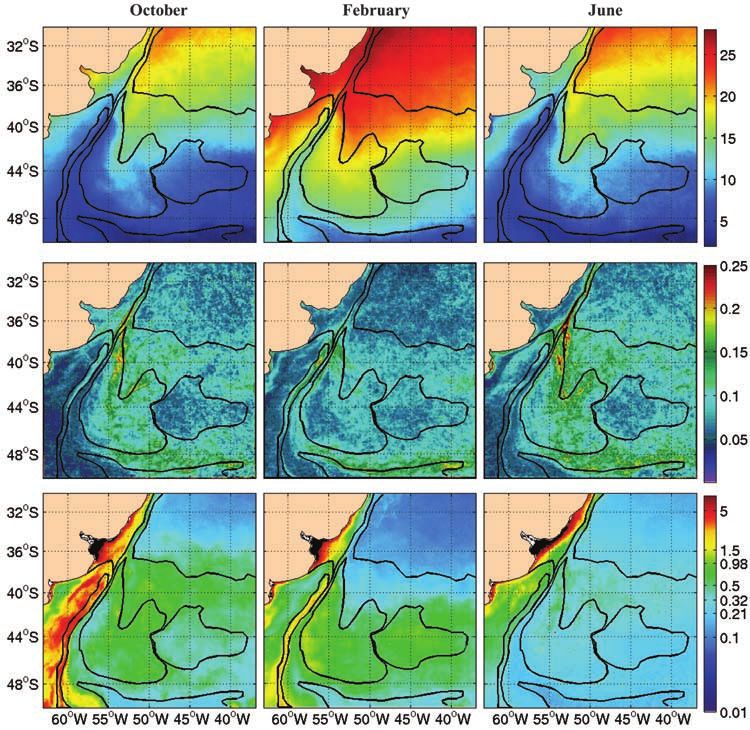
21562202c, 2005, C11, Downloaded from https://agupubs.onlinelibrary.wiley.com/doi/10.1029/2004JC002736 by Cochrane France, Wiley Online Library on [22/02/2023]. See the Terms and Conditions (https://onlinelibrary.wiley.com/terms-and-conditions) on Wiley Online Library for rules of use; OA articles are governed by the applicable Creative Commons License
                  JOURNAL OF GEOPHYSICAL RESEARCH, VOL. 110, C11016, doi:10.1029/2004JC002736, 2005

On the relationship between satellite-retrieved surface
temperature fronts and chlorophyll a
in the western South Atlantic
Martin Saraceno and Christine Provost
Laboratoire d’Océanographie Dynamique et de Climatologie, UMR 7617, CNRS, IRD-UPMC-MNHN, Institut Pierre Simon
Laplace, Université Pierre et Marie Curie, Paris, France

Alberto R. Piola
Departamento de Oceanografı́a, Servicio de Hidrografı́a Naval, Buenos Aires, Argentina
Departamento de Ciencias de la Atmósfera y los Océanos, Facultad de Ciencias Exactas y Naturales, Universidad de Buenos
Aires, Buenos Aires, Argentina
Received 1 October 2004; revised 4 June 2005; accepted 29 August 2005; published 18 November 2005.

[1] The time-space distribution of chlorophyll a in the southwestern Atlantic is examined
using 6 years (1998–2003) of sea surface color images from Sea-viewing Wide Field
of View Sensor (SeaWiFS). Chlorophyll a (chl a) distribution is confronted with sea
surface temperature (SST) fronts retrieved from satellite imagery. Histogram analysis of
the color, SST, and SST gradient data sets provides a simple procedure for pixel
classification from which eight biophysical regions in the SWA are identified, including
three new regions with regard to Longhurst (1998) work: Patagonian Shelf Break (PSB),
Brazil Current Overshoot, and Zapiola Rise region. In the PSB region, coastal-trapped
waves are suggested as a possible mechanism leading to the intraseasonal frequencies
observed in SST and chl a. Mesoscale activity associated with the Brazil Current Front
and, in particular, eddies drifting southward is probably responsible for the high chl a
values observed throughout the Brazil Current Overshoot region. The Zapiola Rise is
characterized by a local minimum in SST gradient magnitudes and shows chl a maximum
values in February, 3 months later than the austral spring bloom of the surroundings.
Significant interannual variability is present in the color imagery. In the PSB, springs and
summers with high chl a concentrations seem associated with stronger local northerly
wind speed, and possible mechanisms are discussed. Finally, the Brazil-Malvinas front is
detected using both SST gradient and SeaWiFS images. The time-averaged position of the
front at 54.2°W is estimated at 38.9°S and its alongshore migration of about 300 km.
Citation: Saraceno, M., C. Provost, and A. R. Piola (2005), On the relationship between satellite-retrieved surface temperature fronts
and chlorophyll a in the western South Atlantic, J. Geophys. Res., 110, C11016, doi:10.1029/2004JC002736.

1. Introduction                                                             and changes in chl a concentration can be used to delineate
1.1. Sea Surface Temperature Fronts and Color                               boundaries of eddies or currents, i.e., oceanic fronts [Quartly
Satellite Images                                                            and Srokosz, 2003]. Fronts are locally marked by high levels
  [2] Since September 1997 the ocean color sensor Sea-                      of chlorophyll a when the mixing between two adjacent
viewing Wide Field of View Sensor (SeaWiFS) has been                        water masses provides the optimal conditions for growth
providing an outstanding data set for a wide range of studies,              (nutrients, light, warmth and enhanced mixing and upwell-
involving large-scale oceanic biological productivity. Chlo-                ing) that neither water masses contain alone [Quartly and
rophyll abundance is associated with fronts, eddies and                     Srokosz, 2003]. The objective of the present paper is to
regions of upwelling. Thus SeaWiFS records are useful for                   compare chl a distribution with SST and SST gradient fields
studying physical processes in the ocean [e.g., McGillicuddy                in the southwestern Atlantic (SWA) Ocean using satellite
et al., 1998; Fratantoni and Glickson, 2002].                               data. Highest values in SST gradient fields are used as a
  [3] In this article, we use chlorophyll a (chl a) as a water              proxy for the surface thermal fronts. The SWA stands out as
mass tracer. Although chl a is a nonconservative quantity,                  one of the regions of the world ocean with highest concen-
near surface chl a concentrations are more or less homoge-                  tration and most complex distribution of chl a. The high
neous within a given water body (a given current or an eddy)                concentration of chl a is associated with high primary
                                                                            productivity, and a major fishery [Food and Agricultural
                                                                            Organization, 1972]. Improving our knowledge on the
Copyright 2005 by the American Geophysical Union.                           spatial distribution of chl a and on the relationship
0148-0227/05/2004JC002736                                                   between chl a and SST fronts is crucial for living

                                                                     C11016                                                        1 of 16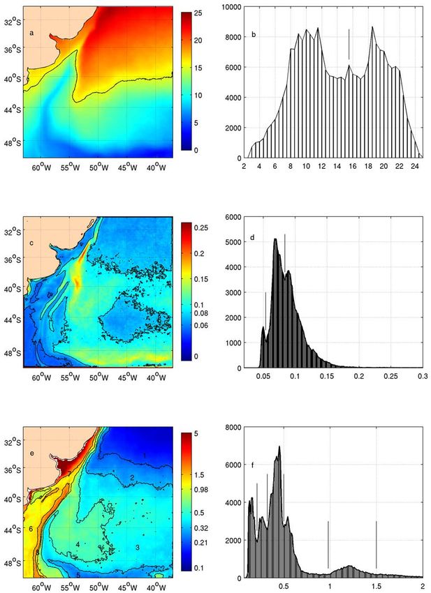
21562202c, 2005, C11, Downloaded from https://agupubs.onlinelibrary.wiley.com/doi/10.1029/2004JC002736 by Cochrane France, Wiley Online Library on [22/02/2023]. See the Terms and Conditions (https://onlinelibrary.wiley.com/terms-and-conditions) on Wiley Online Library for rules of use; OA articles are governed by the applicable Creative Commons License
C11016                SARACENO ET AL.: FRONTS AND CHLOROPHYLL A IN THE SW ATLANTIC                                     C11016

                                                               concentration in the Confluence region reflects the complex
                                                               ocean circulation patterns of the SWA. The Confluence is
                                                               formed by the collision between the Malvinas Current
                                                               (MC) and the Brazil Current (BC) approximately at 38°S
                                                               (Figure 1) and makes the region one of the most energetic
                                                               of the world ocean [Gordon, 1981; Chelton et al., 1990].
                                                               The MC is part of the northern branch of the Antarctic
                                                               Circumpolar Current [Piola and Gordon, 1989] that carries
                                                               the cold and relatively fresh subantarctic water equator-
                                                               ward along the western edge of the Argentine Basin. The
                                                               BC flows poleward along the continental margin of South
                                                               America as part of the western boundary current of the
                                                               South Atlantic subtropical gyre. After its collision with the
                                                               MC, the BC flows southward and, at about 44°S, returns
                                                               to the NE. This path is commonly referred to as the
                                                               overshoot of the Brazil Current [e.g., Peterson and
                                                               Stramma, 1991].
                                                                 [5] Two major oceanic fronts are present in the SWA: the
                                                               Subantarctic Front (SAF) and the Brazil Current Front
                                                               (BCF). The former is the northern boundary of subantarctic
                                                               water and the latter is the southern limit of South Atlantic
Figure 1. Schematic diagram of major fronts and currents       Central Water. Bottom topography plays an important role
in the western South Atlantic. The collision between the       controlling the location of the SAF. The Shelf Break Front
Malvinas Current (MC) and Brazil Current (BC) occurs           and the Malvinas Return Front are part of the SAF and
near 38°S. After collision with the BC, the main flow of the   correspond respectively to the western and eastern bound-
MC describes a sharp cyclonic loop, forming the Malvinas       aries of the MC: their position is established by the sharp
Return Flow (MRF). The mean positions of the Brazil            bottom slope at the shelf edge following approximately the
Current Front (BCF, solid line) and the Subantarctic Front     300 and 3000 m depths, respectively [Saraceno et al., 2004]
(SAF, dash-dotted line) are from Saraceno et al. [2004].       (Figure 1). Bathymetry is also responsible for the low SST
The different shaded regions are from Longhurst’s [1998]       gradient magnitude observed above the Zapiola Rise
biophysical provinces in the southwestern Atlantic (SWA):      [Saraceno et al., 2004]. The position where the Brazil and
South Atlantic Gyral Province (SATL), Brazil Current           Malvinas currents collide is not controlled by bottom topog-
Costal Province (BRAZ), Southwest Atlantic Shelves             raphy and the variability of the position of the resulting front
Province (FKLD), South Subtropical Convergence Province        is a subject of controversial results. Using AVHRR data from
(SSTC), and Subantarctic Water Ring Province (SANT).           1981 to 1987, Olson et al. [1988] estimate that the separation
Isobaths at 300, 3000, 5000, 5250, and 5500 m are              points of the BCF and SAF from the 1000 m isobath occurs
represented [from Smith and Sandwell, 1994]. The Zapiola       around 35.8 ± 1.1°S and 38.6 ± 0.9°S respectively. Using a
Rise feature is observed at 45°W, 45°S. The along- and         combination of altimeter and thermocline depth data, Goni
cross-shelf sections (solid black segments) used to plot the   and Wainer [2001] find that in the period 1993 – 1998 the
Hovmoller diagrams in Figures 5 and 13 are also indicated.     separation of the BCF from the 1000 m isobath depth occurs,
Letters indicate the intersection between the cross-shelf      on average, at 38.5 ± 0.8°S. Computing SST frontal prob-
section and the shelf break front (A), the Malvinas Return     abilities from nine years of AVHRR data, Saraceno et al.
Front (B), and the BCF (C and D). These points correspond      [2004] find evidence that the SAF and BCF merge into a
to local maxima in SST gradient and chl a along the section    single surface front in the collision region. In the lee of the
(Figure 5).                                                    collision region (east of 53.5°W) the two fronts diverge
                                                               (Figure 1) [Gordon and Greengrove, 1986; Roden, 1986]. In
                                                               the collision region, the single front pivots seasonally,
resources management. High fishery activity is present in      around a fixed point located at 39.5°S, 53.5°W [Saraceno
the frontal regions [e.g., Bisbal, 1995]. In particular, the   et al., 2004]. In winter the front is orientated N-S along
Patagonian shelf break has been shown to be an economic        53.5°W and in summer it shifts to a NW-SE direction.
and ecologically important region where the presence of        Because this front separates water masses with distinct
species such as anchovy (E. anchoita) or hake (M. hubbsi)      thermohaline and nutrient characteristics, the frontal dis-
during 5– 6 months of the year are associated with the         placements produce a strong impact on the distribution of
Patagonian shelf break front [Acha et al., 2004]. The large    biota [e.g., Brandini et al., 2000]. Thus the Brazil/Malvinas
primary productivity is also likely to affect the regional     frontal motion should be detectable in satellite color images,
balance of CO2 on the Patagonian shelf [Bianchi et al.,        possibly providing independent evidence of the frontal
2005].                                                         displacements.
                                                               1.2.2. Biophysical Regions
1.2. Southwestern Atlantic Ocean                                 [6] Chl a concentration can be used to identify biogeo-
1.2.1. Physical Characteristics                                graphical regions in the ocean. Longhurst [1998] (hereinaf-
  [4] The SWA Ocean is characterized by the Brazil/            ter referred to as L98) discusses concisely the large-scale chl
Malvinas Confluence region. The distribution of the chl a      a distributions and the major forcing responsible for the chl

                                                          2 of 16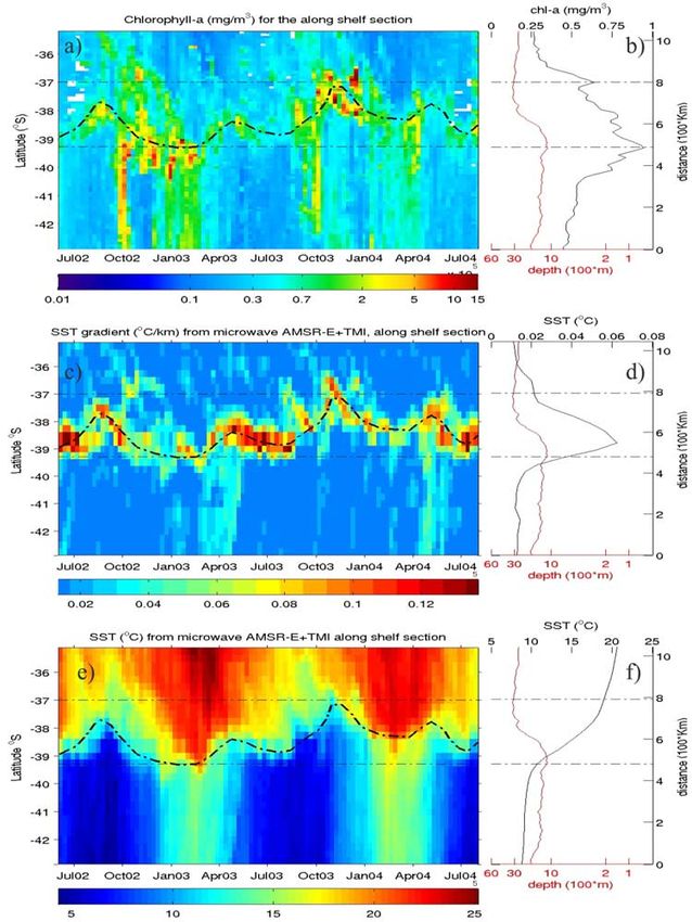
21562202c, 2005, C11, Downloaded from https://agupubs.onlinelibrary.wiley.com/doi/10.1029/2004JC002736 by Cochrane France, Wiley Online Library on [22/02/2023]. See the Terms and Conditions (https://onlinelibrary.wiley.com/terms-and-conditions) on Wiley Online Library for rules of use; OA articles are governed by the applicable Creative Commons License
C11016                 SARACENO ET AL.: FRONTS AND CHLOROPHYLL A IN THE SW ATLANTIC                                     C11016

a concentration in each biogeochemical province that he           Center (GSFC) Distributed Active Archive Center (DAAC)
defined. L98 determines provinces considering several data-       with reprocessing 4 [McClain et al., 1998]. The bins
bases: chlorophyll fields obtained from the coastal zone          correspond to approximately 9  9 km grid cells on a
color scanner (CZCS) sensor, global climatologies of mixed        global grid.
layer depth, Brunt-Väisälä frequency, Rossby internal radius     [10] The RSMAS data set cover the period from January
of deformation, photic depth and surface nutrient concen-         1986 to December 1995. It is composed of 697 images
trations. L98 defines five Provinces in the SWA (Figure 1):       5 day composite with approximately 4  4 km resolu-
The Southwest Atlantic Shelves Province (FKLD) is limited         tion. Cloud detection (G. Podestá, personal communica-
by the 2000 m isobath to the east. Tidal forcing on the shelf     tion, 2004) was done applying a median filter with a
is supposed to be the major forcing of the spring and             window size of 5x5 pixels through the individual images
summer bloom concentrations of chl a (L98). Dynamic               (corresponding to a single pass). All pixels over water
eddying is proposed as the main mechanism causing the             with estimated temperatures below 3°C were flagged as
high concentration values through the shelf break, where a        clouds. Whenever a pixel in the box differed by more
linear chlorophyll feature is observed in a high percentage       than 2°C from the median of the box, it was also
of days, especially in summer (L98). The Brazil Current           flagged as cloud contaminated. Compositing was made
Costal Province (BRAZ) is limited by the 2000 m isobath to        conserving the warmest temperature observed during the
the east and by the confluence between the Brazil and             5 day period for each pixel. This composite reduces the effect
Malvinas currents to the south. A sharp turbidity front           of cloud coverage and the likelihood of negative biases due
marks the limit of tidal stirring near the mouth of the Plata     to cloud contamination [Podestá et al., 1991]. A seasonal
river [Framiñan and Brown, 1996; L98]. The South Atlantic        analysis of the cloud coverage in the SWA using the same
Gyral Province (SATL) comprises the South Atlantic anti-          data set was carried out by Saraceno et al [2004]. It is shown
cyclonic circulation, where surface chlorophyll values are        that the difference between summer and winter cloud cover
low throughout the year over most of the area. The portion        is lower than 10%. Using NCEP (National Center of
of the Subantarctic Water Ring Province (SANT) comprised          Environmental Prediction) and ECWMF (European Centre
in the SWA has an oligotrophic regime. The South Sub-             for Medium Weather Forecasting) reanalysis in the SWA,
tropical Convergence (SSTC) Province presents a strong            Escoffier and Provost [1998] find similar low seasonal
biological enrichment during all seasons (L98).                   variability in cloud cover. Thus we consider that the
                                                                  seasonal cloud cover variability does not affect the results.
1.3. Outline                                                        [11] The RSMAS SST and color time series are not
  [7] After presenting the data and methods in section 2,         concomitant. We consider the 8 day composite with 9
eight biophysical regions are identified based on histogram       9 km of spatial resolution of version 4.1 of the AVHRR
analysis of SST, SST gradient and chl a mean distributions        data from JPL to fill the gap. Version 4.1 assigns excessive
(section 3). The chl a time-space variability and its rela-       cloud coverage in regions with strong thermal gradients
tionship with thermal fronts in the Patagonian Shelf break        [Vazquez et al., 1998]. The front in the Brazil/Malvinas
(PSB), Brazil Current overshoot and Zapiola Rise regions          collision region is constantly covered by ‘‘clouds’’ in those
are examined in section 4. The Brazil-Malvinas collision          images (not shown). Version 4.1 ends on July 2003. The
front as seen with SST gradient and SeaWiFS images is also        latest version (5.1) which spans up-to-date and has a 4
described in section 4. Summary and discussion of the main        4 km spatial resolution presents large regions with constant
results, including further analysis of the chl a interannual      artificial cloud masking in the SWA (as confirmed by
variability, follows in section 5.                                J. Vazquez, personal communication, 2004). Thus we use
                                                                  the 4.1 version to analyze the SST and SST gradient in
                                                                  those regions of the SWA where gradient values are not
2. Data and Methods                                               too high (i.e., in the shelf and shelf break region).
  [8] We use six years (January 1998 to December 2003) of           [12] Because of the lower spatial resolution (one by one
SeaWiFS images and four different sources of satellite            degree), Reynolds data are not adequate to compare the
derived SST based on Advanced Very High Resolution                frontal thermal structures (SST gradient) with color
Radiometer (AVHRR) or microwave measurements. The                 images. However, they are useful when SST time series
AVHRR data used cover different time periods and have             are considered.
different spatial resolution and characteristics according to       [13] Finally, to compare color and SST distributions at the
the processes applied to produce the SST and the cloud            confluence of the Brazil/Malvinas front, AMSR-E [Wentz
masking. The three AVHRR data are (1) data received at a          and Meissner, 2004] data are used. AMSR-E data are
local station in Argentina and processed at the Rosenstiel        available since June 2002 and are cloud free. Their spatial
School of Marine and Atmospheric Science, University of           resolution is about 25 km.
Miami (RSMAS); (2) version 4.1 produced by the Jet                  [14] For each SST image of the RSMAS, 4.1 JPL and
Propulsion Laboratory (JPL), and (3) the optimal interpo-         AMSR-E data set, an SST gradient image is produced
lated data set from Reynolds and Smith [1994]. Microwave          conserving the respective spatial resolution. SST gradient
measurements are from the Advanced Microwave Scanning             magnitude fields were produced using a Prewitt operator
Radiometer for Eos (AMSR-E) [Wentz and Meissner, 2004].           [Russ, 2002] using a window of about 30  30 km
Detailed description of each database follows below.              (corresponding to 7  7 pixels for the RSMAS, 3  3 pixels
  [9] Phytoplankton pigment concentrations are obtained           for the 4.1 JPL and 1  1 pixel for the AMSR-E data set).
from 8 day average composite SeaWiFS products of level 3          This box size retains the large and mesoscale frontal features
binned data, generated by the NASA Goddard Space Flight           with an acceptable amount of noise.

                                                             3 of 16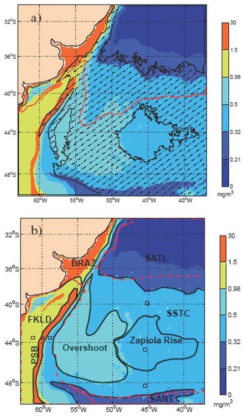
21562202c, 2005, C11, Downloaded from https://agupubs.onlinelibrary.wiley.com/doi/10.1029/2004JC002736 by Cochrane France, Wiley Online Library on [22/02/2023]. See the Terms and Conditions (https://onlinelibrary.wiley.com/terms-and-conditions) on Wiley Online Library for rules of use; OA articles are governed by the applicable Creative Commons License
              C11016
            SARACENO ET AL.: FRONTS AND CHLOROPHYLL A IN THE SW ATLANTIC

                                                                                                                                                                                                                                                                                                                                          Figure 2

                                                                                                                                                                                                                                                                                                                                                      4 of 16
              C11016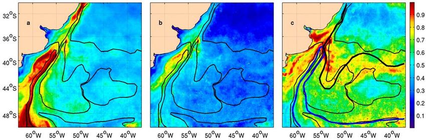
21562202c, 2005, C11, Downloaded from https://agupubs.onlinelibrary.wiley.com/doi/10.1029/2004JC002736 by Cochrane France, Wiley Online Library on [22/02/2023]. See the Terms and Conditions (https://onlinelibrary.wiley.com/terms-and-conditions) on Wiley Online Library for rules of use; OA articles are governed by the applicable Creative Commons License
C11016                 SARACENO ET AL.: FRONTS AND CHLOROPHYLL A IN THE SW ATLANTIC                                         C11016

Table 1. Classification of SST, SST Gradient, and chl a               Centered at 45°S, 45°W, the Zapiola Rise is a region with
According to the Respective Histograms for the Mean Images            low SST gradients. Thresholds determined from the SST
                                                Thresholds            gradient histogram define three distinct ranges (Table 1).
SST, °C                                  16
                                                                      Values over the Zapiola Rise range between 0.06 and
Grad SST, °C/km                          0.06, 0.08                   0.08°C/km. The BCF, the Shelf Break Front and the
Chl a mg/m3                              0.21, 0.32, 0.5, 0.88, 1.5   Malvinas Return Front north of 45°S and the SAF south
                                                                      of 47°S present values higher than 0.08°C/km. Values
                                                                      lower than 0.06°C/km are found in small regions, mostly
  [15] In order to calculate spectra of SST time series               located in the southwest of the domain.
extracted at certain locations (section 4.1), cloudy pixels             [20] The 6 years mean color distribution from SeaWiFS
in the time series are filled using a cubic spline interpola-         shows a wide range of chlorophyll values in the SWA: from
tion. Cloudy pixels in the time series represent less than 8%         oligotrophic regions to regions that exhibits concentrations
of the record length. Spectra, confidence limits (CL) and             higher than 5 mg/m3. The histogram presents five local
significant peaks of the time series are then calculated using        minima or thresholds (Table 1) that classify pixels into six
the singular spectrum analysis multitaper method toolkit              different ranges of values that establish eight major areas in
[Ghil et al., 2002]. Two data tapers are used and signif-             the SWA (Figure 2e).
icant peaks have been estimated with the hypothesis of a                [21] The superposition of the regions derived from the
harmonic process drawn back in a background red noise.                threshold classification shows that most of the boundaries
  [16] To investigate possible forcing mechanisms for the             defined by the SST gradient regions are common with the
variability observed in chl a, surface wind data were                 boundaries of the regions defined by chl a (Figure 3a).
analyzed. We consider satellite scatterometer data from               Eight biophysical regions (Figure 3b) present one or more
QuikSCAT between January 2000 and December 2003                       variables that identify each region uniquely (Table 2). Chl a
(http://www.ifremer.fr/cersat/fr/data/overview/gridded/               defines main regions and the SST threshold separates those
mwfqscat.htm). The wind satellite data are daily and have a           that have common chl a concentrations: PSB from BRAZ
spatial resolution of 0.5°.                                           and SATL from SANT. In addition, the 0.08°C/km gradient
                                                                      threshold is critical to identify the Zapiola Rise. Three of
3. Identification of Regions                                          these regions coincide with the L98 classification into
                                                                      Provinces (SANT, BRAZ and SATL) and three new regions
  [17] The 10 year mean of SST and SST gradient fields                appear, which subdivide the SSTC and FKLD Provinces
from RSMAS and the 6 year mean of chl a fields together               into subregions (Figure 3 and Table 2). The SSTC Province
with their respective histograms (Figure 2) are used to               contains the Zapiola Rise and the Overshoot regions; and
identify biophysical regions in the SWA. Histogram analy-             the FKLD Province contains the PSB region.
sis is largely used in image analysis for objective pixel               [22] The regions identified in this section arise from the
classification [e.g., Russ, 2002]. Histograms of mean images          mean fields, thus variability on interannual or seasonal
(Figures 2b, 2d, and 2f) show that chl a and SST gradient             timescale is not considered. The spatiotemporal variability
magnitude have a multimodal structure, while SST can be               of the chl a and its relationship with thermal fronts is
considered as bimodal. The local minima in the histograms             discussed in the next section; the evolution of the bound-
determine the thresholds used to classify pixels in the mean          aries of biophysical regions with time deserves further
images (Table 1).                                                     analysis and will be the subject of a future work.
  [18] The 10 year RSMAS SST mean (Figure 2a) encom-
passes values from 2°C in the south to 25°C in the north.
Isotherms present strong curvatures associated with the               4. Specific Features
convoluted paths of the Malvinas and Brazil currents (see               [23] In the previous section, three new regions with
Figure 1). The corresponding histogram separates SST in               regard to L98 Provinces were identified. Below we describe
relatively warm (>16°C) and cold (
21562202c, 2005, C11, Downloaded from https://agupubs.onlinelibrary.wiley.com/doi/10.1029/2004JC002736 by Cochrane France, Wiley Online Library on [22/02/2023]. See the Terms and Conditions (https://onlinelibrary.wiley.com/terms-and-conditions) on Wiley Online Library for rules of use; OA articles are governed by the applicable Creative Commons License
C11016 SARACENO ET AL.: FRONTS AND CHLOROPHYLL A IN THE SW ATLANTIC C11016
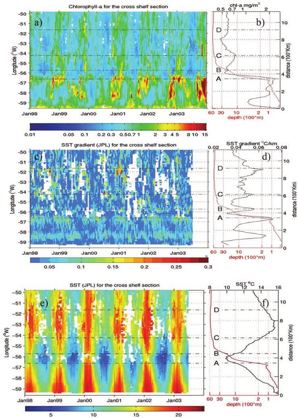
The PSB region is clearly visible in the cross-shelf section
(Figure 5) associated with the local maxima of chl a and
SST gradient at 56.6°W. Both local maxima correspond
in time and space and are located over the topographic
shelf break, emphasizing the strong topographic control
(Figure 5).
[25] Over the shelf and in the core of the MC (west and
east of the PSB region respectively) the time evolution of
the chl a is quite different (Figure 6). Chl a concentra-
tions start increasing in September in the three time series.
From August to April, the PSB region presents higher
concentration with regard to surrounding waters. Values
over the shelf and at the PSB reach their maximum in
October (3.5 mg/m3) while values in the MC reach their
maximum in September and decay to a mean value of
0.5 mg/m3 during the rest of the year. Thus the presence
of the shelf break front is responsible for the higher chl a
values over the PSB region. Different processes associated
with the shelf break front could induce a vertical circula-
tion [Huthnance, 1995] that may enhance a higher trans-
port of nutrients to the euphotic zone than over the
Patagonian shelf or in the MC. To date, such a process
in the PSB region has not been documented in the
literature, while several propositions were made. Erickson
et al. [2003] suggested that iron can be transported from
the South American continent by westerly winds and
fertilize the adjacent South Atlantic Ocean. This kind of
fertilization affects large areas and is therefore unlikely to
explain by itself the higher productivity over the narrow
PSB region. L98 proposed that enhanced topographically
driven mesoscale activity (i.e., eddies) could also play a
role in generating the higher values observed over the PSB
region. However, the higher percentage of eddies that
creates at the B/M Collision region drift southeastward
rather than westward [Lentini et al., 2002] and there is no
evidence of eddies reaching the PSB region. Acha et al.
[2004] additionally suggested that internal waves, coupled
with episodic wind stress, are a possible mechanism to
Figure 3. (a) Six ranges of chl a magnitudes based on the enhance the supply of the nutrient-rich MC to the euphotic
respective histogram, represented by background colors. zone. Finally, Podestá [1990] suggested that the interleaving
The hatched region indicates areas with SST gradients of water masses at the front could enhance vertical stability,
higher than 0.08°C/km. The solid red line is the threshold retaining phytoplankton cells in the euphotic zone.
deduced from the SST field. (b) Information from the three 4.1.1. Seasonal and Intraseasonal Variability
mean fields (SST, chl a, and SST gradient) synthesized and [26] Power spectral density of SST and chl a time series
compared to L98 mean definition of Provinces in the SWA extracted in a box of one by one degree in the northern part
Ocean, with background colors as in Figure 3a. Regions of the PSB region shows significant peaks centered at the
obtained from histograms are indicated with solid black annual and intraseasonal frequencies (Figure 7). The annual
lines, and L98 provinces (BRAZ, SSTC, SANT, SATL, peak is a common factor for the whole region, and has
FKLD) are indicated with dashed red lines. Small boxes already been described both for the SST [e.g., Podestá et
north, south, and within the Zapiola Rise Region and east, al., 1991; Provost et al., 1992] and for the chl a [e.g., L98;
west, and within the Patagonian Shelf Break (PSB)
indicate the position where time series are extracted
(Figures 6 and 12). Table 2. Southwest Atlantic Regional Characteristics
L98 chl a, SST
Region Province mg/m3 SST °C Gradient, °C/km
south of the domain along the western branch of the SAF SATL SATL 16 0.08
this bloom (>0.08°C/km north of 44°S, Figure 3) corre- Overshoot SSTC 0.5 – 0.98 0.08
Zapiola Rise SSTC 0.32 – 0.521562202c, 2005, C11, Downloaded from https://agupubs.onlinelibrary.wiley.com/doi/10.1029/2004JC002736 by Cochrane France, Wiley Online Library on [22/02/2023]. See the Terms and Conditions (https://onlinelibrary.wiley.com/terms-and-conditions) on Wiley Online Library for rules of use; OA articles are governed by the applicable Creative Commons License
C11016 SARACENO ET AL.: FRONTS AND CHLOROPHYLL A IN THE SW ATLANTIC C11016
Figure 4. October, February, and June monthly climatologies of (top) SST (°C), (middle) SST
gradient (°C/km), and (bottom) chl-a (mg/m3). Black lines are limits of biophysical regions as defined
in Figure 3b.
Garcia et al., 2004]. On the other hand, similar intra- [27] The spectra of the SST time series also show a
seasonal peaks than those observed in Figure 7 are present significant peak at the semiannual frequency (Figure 7b).
along the PSB region (and not in adjacent regions, not Using shorter SST time series, Provost et al. [1992] showed
shown) for the SST and chl a time series, suggesting that a that the ratio of the semiannual to the annual component in
process linked to the shelf break is responsible for the the PSB region represents a local maximum with reference
observed variability. We suggest that continental trapped to waters east and west of the shelf break. The semiannual
waves (CTWs) could be the forcing mechanism. CTWs frequency is associated with the semiannual wave present in
were already proposed to be present in the Patagonian shelf the atmosphere at high southern latitudes [Provost et al.,
break by Vivier et al. [2001] to explain the 70 day fluctua- 1992]. The semiannual peak is not significant in the chl a
tions observed in the Malvinas Current transport and in time series (Figure 7a).
SLA at 40°S [Vivier and Provost, 1999]. On the other hand, 4.1.2. Interannual Variability
SSTs could be related to CTWs: along the coast of northern [28] Chl a concentrations over the Patagonian shelf and
Chile, Hormazabal et al. [2001] show that SSTs are shelf break present strong interannual variations (Figure 5).
strongly modulated by CTWs. Thus we suggest that CTWs An overall trend of the spring concentrations to higher
could be the forcing mechanism of the intraseasonal vari- values is observed in the shelf and shelf break region
ability observed in the SST and color satellite data in the (Figure 8). In particular, in the austral spring of 2003, chl
PSB region. This hypothesis supports the suggestion of a concentrations reach values twice higher than the con-
internal waves made by Acha et al. [2004] to explain the centrations observed during spring of previous years. In
higher values of chl a over the PSB. Further analyses are 1999, the spring bloom was present only during the first
necessary to confirm the CTWs hypothesis or find other weeks of the season. To search the origin of the observed
mechanisms to explain the intraseasonal variability observed variability, we focus on the spring part of the time series of
and its origin. For instances, local wind do not seem to be the time concomitant SST anomalies, meridional and zonal
related to CTWs: meridional and zonal components of the wind speed. SST anomalies and zonal wind speed do not
local wind do not show significant intraseasonal periodicities exhibit any clear relationship with the chl a time series
(not shown). (Figure 9). On the other hand, the meridional wind speed
7 of 1621562202c, 2005, C11, Downloaded from https://agupubs.onlinelibrary.wiley.com/doi/10.1029/2004JC002736 by Cochrane France, Wiley Online Library on [22/02/2023]. See the Terms and Conditions (https://onlinelibrary.wiley.com/terms-and-conditions) on Wiley Online Library for rules of use; OA articles are governed by the applicable Creative Commons License
C11016 SARACENO ET AL.: FRONTS AND CHLOROPHYLL A IN THE SW ATLANTIC C11016
Figure 5. (a) Chl a (mg/m3), (c) SST gradient (°C/km), and (e) SST (°C) versus time for the cross-shelf
section. The position of the section is indicated in Figure 1. The bathymetry and the time average of the
(b) chl a, (d) SST gradient, and (f) SST along the section is plotted to the right of the Hovmoller diagrams.
Local chl a maxima are indicated with dash-dotted lines and reported on the SST and SST gradient
sections. Chl a local maxima correspond to the intersection with the shelf break front (A), Malvinas
Return front (B), and western (C) and eastern (D) branches of the BCF (see Figure 1). The local minima
in three sections between points A and B correspond to the core of the Malvinas Current. White pixels on
the Hovmoller diagrams indicate cloud-covered regions. Cloud coverage is higher in the overshoot region
(between C and D) because the cloud-masking algorithm used by JPL assigns excessive masking to
regions with high SST gradients [Vazquez et al., 1998].
could explain part of the interannual variability: from concentrations observed. Further, data suggest that the
September to December, northerly winds are higher in occurring date of the spring blooms is affected by the
2002 and 2003 than in 2000 and 2001 (Figure 10), direction of the meridional wind speed (Figure 10): when
corresponding respectively to the highest and lowest chl a southerly winds prevailed (i.e., late August and early
8 of 1621562202c, 2005, C11, Downloaded from https://agupubs.onlinelibrary.wiley.com/doi/10.1029/2004JC002736 by Cochrane France, Wiley Online Library on [22/02/2023]. See the Terms and Conditions (https://onlinelibrary.wiley.com/terms-and-conditions) on Wiley Online Library for rules of use; OA articles are governed by the applicable Creative Commons License
C11016 SARACENO ET AL.: FRONTS AND CHLOROPHYLL A IN THE SW ATLANTIC C11016
Figure 6. Chl a time series from the continental shelf (solid line), PSB (dotted line), and MC (dashed
line). The location of the points where time series are extracted is indicated on Figure 3b. Each value in
the time series is the monthly mean within a 30 km 30 km box.
September 2000 and 2002) the spring bloom occurred and its southern part is centered approximately at 54°W,
during the first days of October. Conversely, when northerly 44°S (Figures 1, 2, and 4). The western and eastern
winds prevailed (i.e., late August and early September 2001 branches of the BCF are observed as two local maxima
and 2003), the spring bloom took place during the first days centered at 54.2°W and 51.6°W in the cross-shelf SST
of September. gradient and chl a sections (Figures 5d and 5b). Thus the
[29] These observations further suggest that stronger concentration of chl a is enhanced along the BCF. The
northerly winds lead to higher chl a concentrations over overshoot region is also characterized by warmer temper-
the Patagonian shelf and shelf break regions. Northerly atures with reference to adjacent regions (Figure 5e). The
winds induce an eastward Ekman water mass transport in advection of eddies coming from the BC are responsible for
the southern hemisphere. The Ekman transport of the strat- the higher temperatures. The mesoscale activity associated
ified shelf waters to the nutrient-rich waters of the Malvinas with the front and in particular eddies that drift southward
Current may result in the interleaving of the different water are probably responsible for the high chl a values observed
masses at the shelf break front that could enhance vertical throughout the overshoot region. Chl a concentrations are
stability, retaining phytoplankton cells in the euphotic zone known to be enhanced in high mesoscale activity regions
[Podestá, 1990]. Brandini et al. [2000] have described [L98; Garçon et al., 2001].
similar water interleaving in the Brazil-Malvinas Confluence [32] Not all the overshoot region corresponds to SST
region as the mechanism responsible for the high chl a gradients higher than 0.08°C/km: lower values are present
observed. in a region between the MRF and the BCF (between 42 and
[30] In agreement with our results, Gregg et al. [2005] 47°S and 56 and 57°W, see Figures 3a and 4). In this
also observed a significant positive trend in chl a over the particular region, chl a concentrations reach their maximum
Patagonian shelf. They also found a negative trend in SST values three months later than in the surroundings (Figure 4).
that was associated with increased upwelling. There is no The region corresponds to low eddy kinetic energy values
conflict with our results (Figure 9) because the SST trend compared to the east of the overshoot region (Figure 11)
reported by Gregg et al. [2005] is based on all months of the indicating that fewer eddies are present. This observation is
year, while we just considered spring months. In fact, if all in agreement with the trajectories of eddies observed by
months are considered, we also find a negative trend in SST, Lentini et al. [2002]: eddies generated in the BCF drift
that is associated with lower winter SSTs (not shown). Thus, southeastward rather than westward in the overshoot region.
to sustain the hypothesis of Gregg et al. [2005] for the A lower eddy kinetic energy could explain lower chl a
Patagonian shelf chl a trend, a relation between higher concentrations, but does not explain the 3 month lag of the
winter upwelling and increased spring chl a is required. chl a maximum.
Understanding the relative role of winter upwelling, Ekman
currents or other mechanisms that may lead to enhanced chl 4.3. Zapiola Rise
a concentrations, will require longer term satellite borne and [33] The Zapiola Rise region stands out as a low SST
in situ observations. gradient region throughout the year [Saraceno et al., 2004].
The region extends over 1000 km in the zonal direction and
4.2. Brazil Current Overshoot 600 km in the meridional direction, and closely matches
[31] In the overshoot region, chl a concentrations are the location of the Zapiola Rise, centered at 45°S, 45°W
higher than 1 mg/m3 from September to March (see the (Figure 3).
climatologies for October and February in Figure 4). In [34] Chl a exhibits a local maximum in February and a
austral winter, relatively high chl a concentrations are minimum in October (Figure 4). From October to December
present only near the Brazil Current Front (BCF, see June (January to April), chl a concentrations over the rise are
in Figure 4). The BCF in the overshoot region has a U shape lower (higher), with reference to values north and south of
9 of 1621562202c, 2005, C11, Downloaded from https://agupubs.onlinelibrary.wiley.com/doi/10.1029/2004JC002736 by Cochrane France, Wiley Online Library on [22/02/2023]. See the Terms and Conditions (https://onlinelibrary.wiley.com/terms-and-conditions) on Wiley Online Library for rules of use; OA articles are governed by the applicable Creative Commons License
C11016 SARACENO ET AL.: FRONTS AND CHLOROPHYLL A IN THE SW ATLANTIC C11016
Figure 8. Chl a time series averaged on a 1° box side
centered at 40.25°S, 56.73°W, i.e., in the northern part of
the PSB region.
[35] An anticyclonic flow, with a mean barotropic trans-
port higher than 100 Sv, has been estimated around the
Zapiola Rise [Saunders and King, 1995]. Modeling studies
suggest that the anticyclonic circulation is maintained by
eddy-driven potential vorticity fluxes accelerating the flow
within the closed potential vorticity contours that surround
the rise [de Miranda et al., 1999]. Using altimetry data, Fu
et al. [2001] showed that at intraseasonal scales the closed
Figure 7. Power spectral density of (a) chl a and
(b) RSMAS SST time series extracted in a 1° box side
from the PSB region at 40.25°S, 56.73°W. The power
spectral densities of the JPL SST and Reynolds SST time
series in the same region present similar significant
intraseasonal variability (not shown).
the region (Figure 12). From May to September, chl a
concentrations are low (0.3 mg/m3) and similar to the values
observed further south (Figure 12). Maximum chl a concen-
trations north and south of the rise are reached in November
(Figure 12; see Figure 3 for locations). Dandonneau et al.
[2004] estimate the phase of the annual cycle in SeaWiFS
chl a concentrations using 3 years (1998 – 2001) of monthly
data averaged on a 0.5° longitude 0.5° latitude grid.
Even with these lower spatial resolution and shorter time Figure 9. Spatial average on a 1° box side (centered
record length, the Zapiola Rise reaches its maximum at 40.25°S, 56.73°W) and time mean for austral spring
amplitude in February, in agreement with our analysis. (21 September to 21 December) of SST anomaly (dark blue),
In addition, the Zapiola Rise is a region of relatively chl a (cyan), meridional wind speed (yellow), and zonal
modest eddy kinetic energy, surrounded by areas of very wind speed (brown) for the 4 years (2000– 2003) where data
high eddy energy levels associated with the SAF and BCF are concomitant. SST data are from Reynolds and Smith
mesoscale activity (Figure 11). Thus sea surface height [1994]. The SST anomaly is obtained as the difference
anomaly also suggests that the Zapiola Rise is distinct between the raw data and the fit of a sinusoidal function (in
from the L98 SSTC Province. the less square sense) to the data.
10 of 1621562202c, 2005, C11, Downloaded from https://agupubs.onlinelibrary.wiley.com/doi/10.1029/2004JC002736 by Cochrane France, Wiley Online Library on [22/02/2023]. See the Terms and Conditions (https://onlinelibrary.wiley.com/terms-and-conditions) on Wiley Online Library for rules of use; OA articles are governed by the applicable Creative Commons License
C11016 SARACENO ET AL.: FRONTS AND CHLOROPHYLL A IN THE SW ATLANTIC C11016
Figure 10. Time series of the QuickScat wind speed data averaged on a 1° box side centered at 40.25°S,
56.73°W. Only the August – December period of the 2000 – 2003 time series is shown. Data are low-pass
filtered with a cutoff frequency of 15 days. Solid arrows indicate the beginning of the first strong spring
chl a bloom of the year.
potential vorticity contours provide a mechanism for the and for the RSMAS SST gradient data set (i.e., from
confinement of topographic waves around the Zapiola Rise. January 1985 to December 1995, not shown). The JPL data
These physical mechanisms may cause the dynamical set shows excessive cloud masking in the region (see com-
isolation of the region, and therefore explain the local ments in section 2). In spite of the large interannual vari-
minimum in SST gradient and SLA, but do not explain ability (both in position and magnitude) observed in chl a
why the bloom in the Zapiola Rise occurs in late summer between 1998 and 2003, the front shows in general to shift
and not in spring as in the surrounding areas (Figure 12). northward in late winter and southward in late summer.
The monthly means of the mixed layer depth, as estimated [37] The time average of chl a concentrations on the
by Levitus and Boyer [1994], do not present significant along-shelf section (Figure 13b) shows two local maxima, at
differences over the Zapiola Rise, with reference to the 37 and 39.2°S, which respectively correspond to the north-
surroundings. Hence the stability of the water column does ern and southern limits of the Brazil-Malvinas Collision
not seem to explain the lag between the Zapiola Rise and front. Between these limits, the time average of the SST
the surroundings. However, very few data are available in gradient values also presents the highest values of the
the region to build the monthly means of the mixed layer section (Figure 13d). The time average of the SST section
depth [Levitus and Boyer, 1994]. (Figure 13f) shows clearly that the transition region from
the colder subantarctic waters (8°C) to the warmer Subtrop-
4.4. Brazil-Malvinas Collision front ical waters (> than 18°C) is contained between the limits
[36] In the collision region (i.e., between 53.5 and 55°W previously defined. The inflection point of the curve in
and 37.5 and 40.5°S) the Malvinas and Brazil currents Figure 13f is located at 38.9°S, corresponding also to the
produce a very active front that is identified year-round in latitude of the maximum in the SST gradient time average
SST gradient and ocean color data. Following the along- plot (Figure 13d). Thus we associate this point (54.2°W,
shelf section shown in Figure 1, a time-coincident local 38.9°S) to the time-averaged position of the Brazil-Malvinas
maximum in chl a and SST gradient is observed within the Collision front along the section. The intersection between
northern and southern limits throughout the respective the along-shelf section and the coincident mean positions
record lengths (Figures 13a and 13c). Similar along shore of the SAF and BCF as estimated by Saraceno et al.
frontal displacements are present in chl a concentrations [2004] is in good agreement (Figure 14) with the previous
and SST gradients. Thus it is clear that the chl a concen- observation.
tration increases at the Brazil-Malvinas Collision front. The [38] South of 39.2°S, relatively high chl a values
displacement of the front along the section is also observed (1.2 mg/m3) are usually present from October to April
between the same range of latitudes for the rest of the (austral spring and summer). At that time, a strong bloom
available chl a data (i.e., from January 1998, not shown) over the Patagonian Shelf Break is observed (see section 4.1),
11 of 1621562202c, 2005, C11, Downloaded from https://agupubs.onlinelibrary.wiley.com/doi/10.1029/2004JC002736 by Cochrane France, Wiley Online Library on [22/02/2023]. See the Terms and Conditions (https://onlinelibrary.wiley.com/terms-and-conditions) on Wiley Online Library for rules of use; OA articles are governed by the applicable Creative Commons License
C11016 SARACENO ET AL.: FRONTS AND CHLOROPHYLL A IN THE SW ATLANTIC C11016
Brandini et al., 2000; Garcia et al., 2004]. In particular,
between September and November 2003, this observation
is partly confirmed by the relatively low temperatures
(Figure 13e) that are observed in the same regions where
chl a is higher than normal (Figure 13a) north of 37°S.
[40] The time average of the SST gradient at the along-
shelf section shows a range of about 200 km of maximum
values between 37.6°S and 39°S (Figure 13d). This range
of migration coincides with the separation between the
summer and winter frontal positions derived from SST
frontal probability maps obtained by Saraceno et al.
[2004], which are schematically indicated in Figure 14.
The range of migration of the chl a maximum along the
section is of about 310 km (Figure 13b), exceeding by
55 km at each end of the SST gradient range of migration
(Figure 14). The patchiness of the chlorophyll distribution is
probably responsible of the larger alongshore range of
migration of the chl a maximum with reference to the
SST front. The mechanisms responsible for the observed
motion of the surface expression of the BMF are not
understood. In situ measurements show that the subsurface
Figure 11. Root mean square of sea level anomaly (SLA) orientation of the front in summer is N-S [Provost et al.,
in cm from January 1993 to December 2003. Dash-dotted 1996], matching the surface expression in austral winter.
lines are mean positions of BCF and SAF (as in Figure 1). The relatively strong and shallow (21562202c, 2005, C11, Downloaded from https://agupubs.onlinelibrary.wiley.com/doi/10.1029/2004JC002736 by Cochrane France, Wiley Online Library on [22/02/2023]. See the Terms and Conditions (https://onlinelibrary.wiley.com/terms-and-conditions) on Wiley Online Library for rules of use; OA articles are governed by the applicable Creative Commons License
C11016 SARACENO ET AL.: FRONTS AND CHLOROPHYLL A IN THE SW ATLANTIC C11016
Figure 13. (a) Chl a (mg/m3), (c) SST gradient (°C/km), and (e) SST (°C) versus time for the along-
shelf section. The position of the section is indicated in Figure 1. The bathymetry and the time average of
the (b) chl a, (d) SST gradient and (f) SST along the section are indicated in the plots to the right of the
space-time figures. Chl a local maxima are indicated with dash-dotted lines and reported in the SST and
SST gradient sections.
important in the development of chl a blooms are ubiqui- the Patagonian Shelf Break, the Brazil Current Overshoot
tous features of this part of the southwestern South Atlantic. and the Zapiola Rise. These regions provide a more accurate
The near coincidence between open ocean SST fronts and description of the SWA.
chl a maxima in the collision and overshoot regions [44] 2. Power spectral density of SST and chl a in the
suggests that frontal dynamics plays an important role in PSB region shows significant peaks at intraseasonal
causing the observed blooms in these regions. frequencies. Coastal-trapped waves are suggested as a
[42] The major results and observations from this study possible mechanism leading to the variability observed.
are as follows. [45] 3. Mesoscale activity associated with the BCF and in
[43] 1. Using histogram analysis of mean SST, SST particular eddies drifting southward are probably responsible
gradient and chl a images, we identified three new biogeo- for the high chl a values observed throughout the Brazil
graphical regions with regard to L98 Provinces in the SWA: Current Overshoot region.
13 of 1621562202c, 2005, C11, Downloaded from https://agupubs.onlinelibrary.wiley.com/doi/10.1029/2004JC002736 by Cochrane France, Wiley Online Library on [22/02/2023]. See the Terms and Conditions (https://onlinelibrary.wiley.com/terms-and-conditions) on Wiley Online Library for rules of use; OA articles are governed by the applicable Creative Commons License
C11016 SARACENO ET AL.: FRONTS AND CHLOROPHYLL A IN THE SW ATLANTIC C11016
[Podestá, 1990]. Further analyses and comparison with in
situ data are necessary to asses these hypotheses.
[48] 6. The Brazil-Malvinas front is detected using both
SST gradient and SeaWiFS images. The time-averaged
position of the front at 54.2°W is estimated at 38.9°S and
its alongshore migration of about 300 km. This result agrees
with that of Saraceno et al. [2004]. To describe, and better
understand the potential impact of the frontal movements on
the chlorophyll fields, the analysis of consecutive instanta-
neous and coincident high-resolution SST, SST gradient,
and chl a fields have been undertaken using Moderate-
Resolution Imaging Spectroradiometer (MODIS) data
[Barre et al., 2005].
[49] The important interannual variability in the chl a
fields observed in the two time-space sections and in the time
series (respectively Figures 5, 13, and 8) lead us to estimate
the interannual standard deviation (ISD, equation (1))
Figure 14. Schematic positions of the surface fronts in the and compare it to the monthly standard deviation (MSD,
BM collision region. Summer and winter frontal probability equation (2)) in the SWA, defined as follows:
positions of the BCF and SAF are from Saraceno et al.
[2004]. The dash-dotted line is the 1000 m isobath. The vffiffiffiffiffiffiffiffiffiffiffiffiffiffiffiffiffiffiffiffiffiffiffiffiffiffiffiffiffiffiffiffiffiffiffiffiffiffiffiffiffiffiffiffiffiffiffiffiffiffiffi
2ffi
uX
green segment is the range of migration of the chl a front u chl ð i; j Þ h chl ði Þ i
u j
along the along-shelf section (thin black line). t ij
ISD ¼ ð1Þ
N 1
[46] 4. Chl a maximum in the Zapiola Rise region and in
the southwestern part of the overshoot region is observed in vffiffiffiffiffiffiffiffiffiffiffiffiffiffiffiffiffiffiffiffiffiffiffiffiffiffiffiffiffiffiffiffiffiffiffiffiffiffiffiffiffiffiffiffiffiffiffi
2ffi
uX
February, three months later than in the surrounding waters. u chl ð i; j Þ h chl i
u ij
Mechanisms to explain the delay in the bloom in this t ij
MSD ¼ ð2Þ
region are still unknown. In situ data are necessary to N 1
describe the subsurface structure and understand the
underlying processes. where j spans the 6 years (1998 –2003) of chl a, i spans
[47] 5. Significant interannual variability in chl a over the the 12 months of the year, chl is a matrix containing the
Patagonian shelf break region is observed, especially in 72 (N) monthly means of chl a and the brackets indicate
spring. Highest chl a concentrations seem associated with average over the index (thus hchl(i)ij in A are the monthly
stronger local northerly wind speed that results in an climatologies of chl a and hchliij in B is the mean field of
eastward transport of shelf water to the nutrient-rich waters chl a).
of the Malvinas Current. It is suggested that the resulting [50] The interannual and monthly standard deviation maps
interleaving of water masses may enhance vertical stability and their ratio (ISD/MSD) are presented in Figure 15. The
and thus retains phytoplankton cells in the euphotic zone ISD represents a high portion (higher than 0.7) of the MSD
Figure 15. (a) Monthly chl a standard deviation, (b) interannual chl a standard deviation (see formula
in the text), and (c) ratio of interannual and monthly standard deviation (c = b/a). Log of monthly
means was considered because attenuate the contrast between the higher and lower values. Units in
Figures 15a and 15b are log(mg/m3). The three fields are scaled between 0 and 1. Thin black lines are
contours of the biophysical regions defined in Figure 3. Thick lines in Figure 15c are the SAF (blue)
and BCF (black), as described in Figure 1.
14 of 1621562202c, 2005, C11, Downloaded from https://agupubs.onlinelibrary.wiley.com/doi/10.1029/2004JC002736 by Cochrane France, Wiley Online Library on [22/02/2023]. See the Terms and Conditions (https://onlinelibrary.wiley.com/terms-and-conditions) on Wiley Online Library for rules of use; OA articles are governed by the applicable Creative Commons License
C11016 SARACENO ET AL.: FRONTS AND CHLOROPHYLL A IN THE SW ATLANTIC C11016
in the B/M Collision region and in general along the BCF de Miranda, A. P., B. Barnier, and W. Dewar (1999), On the dynamics of
(Figure 15c). From 36 to 40°S, the highest ratio values the Zapiola Anticyclone, J. Geophys. Res., 104, 21,137 – 21,149.
Erickson, D. J., III, J. L. Hernandez, P. Ginoux, W. W. Gregg, C. McClain,
precisely follows the B/M Collision front (i.e., where the and J. Christian (2003), Atmospheric iron delivery and surface ocean
BCF and SAF coincide), indicating the important interan- biological activity in the Southern Ocean and Patagonian region, Geo-
nual variability of the chl a in that region. High ratio values phys. Res. Lett., 30(12), 1609, doi:10.1029/2003GL017241.
Escoffier, C., and C. Provost (1998), Surface forcing over the southwest
are also present over the FKLD region north of 45°S. In Atlantic from NCEP and ECMWF reanalyses on the period 1979 – 1990,
contrast, the BRAZ region shows high ratio values only at Phys. Chem. Earth, 23, 7 – 8.
the mouth of La Plata River. SATL and Zapiola Rise regions Food and Agricultural Organization (FAO) (1972), Atlas of the Living
Resources of the Sea, Rome.
also show low interannual variability. The PSB and over- Framiñan, M. B., and O. B. Brown (1996), Study of the Rı́o de la Plata
shoot regions show intermediate ratio values, while higher turbidity front. Part I: Spatial and temporal distribution, Cont. Shelf Res.,
ratio values are present over the MC. 16(10), 1259 – 1282.
[51] The results presented here include a wide range of Fratantoni, D. M., and D. A. Glickson (2002), North Brazil Current ring
generation and evolution observed with SeaWiFS, J. Phys. Oceanogr.,
different phenomena. Most of the results are descriptions 32(3), 1058 – 1074.
of simple calculations that raise an important number of Fu, L.-L., B. Cheng, and B. Qiu (2001), 25-day period large-scale oscilla-
unresolved issues in the region, e.g., (1) the important tions in the Argentine Basin revealed by the TOPEX/Poseidon altimeter,
J. Phys. Oceanogr., 31(2), 506 – 517.
interannual chl a variability in almost the whole SWA, Garcia, C. A. E., Y. V. B. Sarma, M. M. Mata, and V. M. T. Garcia (2004),
(2) the mechanism driving the chl a distribution over the Chlorophyll variability and eddies in the Brazil-Malvinas Confluence
Zapiola Rise, (3) the variability of the boundaries of the region, Deep Sea Res., Part II, 51, 159 – 172.
Garçon, V. C., A. Oschlies, S. C. Doney, D. McGillicuddy, and J. Waniek
biophysical regions. As longer time series of satellite data (2001), The role of mesoscale variability on plankton dynamics in the
become available, a more accurate description of the North Atlantic, Deep Sea Res., Part II, 48, 2199 – 2226.
interannual variability will be possible. However, satellite Ghil, M., et al. (2002), Advanced spectral methods for climatic time series,
data alone are not sufficient to measure many aspects of Rev. Geophys., 40(1), 1003, doi:10.1029/2000RG000092.
Goni, G. J., and I. Wainer (2001), Investigation of the Brazil Current front
the relationship between fronts and chl a. Analyses of variability from altimeter data, J. Geophys. Res., 106, 31,117 – 31,128.
satellite and in situ data combined with modeling studies Gordon, A. L. (1981), South Atlantic thermocline ventilation, Deep Sea
should be undertaken to improve our understanding of Res., Part A, 28, 1239 – 1264.
Gordon, A. L., and C. L. Greengrove (1986), Geostrophic circulation of the
phytoplankton bloom dynamics in the SWA. Brazil-Falkland Confluence, Deep Sea Res., Part A, 573 – 585.
Gregg, W. W., N. W. Casey, and C. R. McClain (2005), Recent trends in
[52] Acknowledgments. The Goddard Space Flight Center (GSFC/ global ocean chlorophyll, Geophys. Res. Lett., 32, L03606, doi:10.1029/
NASA) provided the SeaWiFS data used in this work. AVHRR data 2004GL021808.
described as from RSMAS were collected by Servicio Meteorológico Hormazabal, S., G. Shaffer, J. Letelier, and O. Ulloa (2001), Local and
Nacional, Fuerza Aérea Argentina, as part of a cooperative study of that remote forcing of sea surface temperature in the coastal upwelling system
organization with the University of Miami. V. Garçon provided many useful off Chile, J. Geophys. Res., 106, 16,657 – 16,672.
comments on an earlier version of the manuscript. Discussions with Huthnance, J. M. (1995), Circulation, exchange and water masses at the
Y. Dandonneau about chl a distribution on the Zapiola-Rise are duly ocean margin: The role of physical processes at the shelf edge, Prog.
acknowledged. M.S. is supported by a fellowship from Consejo Nacional Oceanogr., 35(4), 353 – 431.
de Investigaciones Cientı́ficas y Técnicas (Argentina). A.R.P. was sup- Legeckis, R., and A. L. Gordon (1982), Satellite-observations of the Brazil
ported by grant CRN-61 from the Inter-American Institute for Global and Falkland Currents— 1975 to 1976 and 1978, Deep Sea Res., Part A,
Change Research and PICT99 07-06420 from Agencia Nacional de 29, 375 – 401.
Promoción Cientı́fica y Tecnológica, Argentina. Constant support from Lentini, C. A. D., D. B. Olson, and G. P. Podestá (2002), Statistics of Brazil
CNES (Centre National d’Etudes Spatiales) is acknowledged. Current rings observed from AVHRR: 1993 to 1998, Geophys. Res. Lett.,
29(16), 1811, doi:10.1029/2002GL015221.
Levitus, S., and T. Boyer (1994), World Ocean Atlas 1994, vol. 4,
References Temperature, NOAA Atlas NESDIS 4, NOAA, Silver Spring, Md.
Acha, E. M., H. W. Mianzan, R. A. Guerrero, M. Favero, and J. Bava Longhurst, A. (1998), Ecological Geography of the Sea, Elsevier, New
(2004), Marine fronts at the continental shelves of austral South York.
America—Physical and ecological processes, J. Mar. Syst., 44, 83 – 105. Martos, P., and M. C. Piccolo (1988), Hydrography of the Argentine
Barre, N., C. Provost, and M. Saraceno (2005), Spatial and temporal scales continental shelf between 38° and 42°S, Cont. Shelf Res., 8(9),
of the Brazil-Malvinas Confluence region documented by MODIS high 1043 – 1056.
resolution simultaneous SST and color images, Adv. Space Res., in press. McClain, C. R., M. L. Cleave, G. C. Feldman, W. W. Gregg, S. B. Hooker,
Bianchi, A. A., C. F. Giulivi, and A. R. Piola (1993), Mixing in the and N. Kuring (1998), Science quality SeaWiFS data for global biosphere
Brazil/Malvinas Confluence, Deep Sea Res., 40, 1345 – 1358. research, Sea Technol., 39(9), 10 – 16.
Bianchi, A. A., A. R. Piola, and G. Collino (2002), Evidence of double- McGillicuddy, D. J., Jr., A. R. Robinson, D. A. Siegel, H. W. Jannasch,
diffusion in the Brazil/Malvinas Confluence, Deep Sea Res., Part I, 49, R. Johnson, T. D. Dickey, J. McNeil, A. F. Michaels, and A. H. Knap
41 – 52. (1998), Influence of mesoscale eddies on new production in the Sargasso
Bianchi, A. A., L. Biancucci, A. R. Piola, D. Ruiz Pino, I. Schloss, A. R. Sea, Nature, 394, 263 – 266.
Poisson, and C. F. Balestrini (2005), Vertical stratification and air-sea Olson, D. B., G. P. Podesta, R. H. Evans, and O. B. Brown (1988), Tem-
CO 2 fluxes in the Patagonian shelf, J. Geophys. Res., C07003, poral variations in the separation of Brazil and Malvinas Currents, Deep
doi:10.1029/2004JC002488. Sea Res., Part A, 35, 1971 – 1990.
Bisbal, G. (1995), The southeast South American shelf large marine Peterson, R. G., and L. Stramma (1991), Upper-level circulation in the
ecosystem: Evolution and components, Mar. Policy, 19, 21 – 38. South Atlantic Ocean, Prog. Oceanogr., 26(1), 1 – 73.
Brandini, F. P., D. Boltovskoy, A. Piola, S. Kocmur, R. Rottgers, P. Cesar Piola, A. R., and A. L. Gordon (1989), Intermediate waters of the western
Abreu, and R. Mendes Lopes (2000), Multiannual trends in fronts and South Atlantic, Deep Sea Res., 36, 1 – 16.
distribution of nutrients and chlorophyll in the southwestern Atlantic Podestá, G. P. (1990), Migratory pattern of Argentine hake Merluccius
(30 – 62°S), Deep Sea Res., Part I, 47, 1015 – 1033. hubbsi and oceanic processes in the southwestern Atlantic Ocean, Fish.
Chelton, D. B., M. G. Schlax, D. L. Witter, and J. G. Richman (1990), Bull., 88(1), 167 – 177.
GEOSAT altimeter observations of the surface circulation of the Southern Podestá, G. P., O. B. Brown, and R. H. Evans (1991), The annual cycle of
Ocean, J. Geophys. Res., 95, 17,877 – 17,903. satellite-derived sea surface temperature in the southwestern Atlantic
Dandonneau, Y., P.-Y. Deschamps, J.-M. Nicolas, H. Loisel, J. Blanchot, Ocean, J. Clim., 4, 457 – 467.
Y. Montel, F. Thieuleux, and G. Becu (2004), Seasonal and interannual Provost, C., O. Garcia, and V. Garçon (1992), Analysis of satellite sea
variability of ocean color and composition of phytoplankton commu- surface temperature time series in the Brazil-Malvinas Current confluence
nities in the North Atlantic, equatorial Pacific and South Pacific, Deep region: Dominance of the annual and semiannual periods, J. Geophys.
Sea Res., Part II, 51, 303 – 318. Res., 97, 17,841 – 17,858.
15 of 16You can also read