On Wire-Grid Representation for Modeling Symmetrical An- tenna Elements - Preprints
←
→
Page content transcription
If your browser does not render page correctly, please read the page content below
Preprints (www.preprints.org) | NOT PEER-REVIEWED | Posted: 6 June 2022                              doi:10.20944/preprints202206.0061.v1

     Article

     On Wire-Grid Representation for Modeling Symmetrical An-
     tenna Elements
     Adnan Alhaj Hasan 1*, Dmitriy V. Klyukin 1, Aleksey A. Kvasnikov 1, Maxim E. Komnatnov 1
     and Sergei P. Kuksenko 1

                                       1 Scientific Research Laboratory of Basic Research on Electromagnetic Compatibility, Tomsk State University
                                         of Control Systems and Radioelectronics, 634050 Tomsk, Russia; alhaj.hasan.adnan@tu.tusur.ru (A.A.H);
                                         dv_klyukin@tu.tusur.ru (D.V.K.); aleksejkvasnikov@tu.tusur.ru (A.A.K.); maxmek@mail.ru (M.E.K.);
                                         ksergp@tu.tusur.ru (S.P.K.).
                                       * Correspondence: alhaj.hasan.adnan@tu.tusur.ru.

                                       Abstract: This paper focuses on the combination of the method of moments and the wire-grid ap-
                                       proximation as an effective computational technique for modeling symmetrical antennas with low
                                       computational cost and quite accurate results. The criteria and conditions for the use of wire-grid
                                       surface approximation from various sources are presented together with new recommendations for
                                       modeling symmetrical antenna structures using the wire-grid approximation. These recommenda-
                                       tions are used to calculate the characteristics of biconical and horn antennas at different frequencies.
                                       The results obtained using different grid and mesh settings are compared to those obtained analyt-
                                       ically. Moreover, the results are compared to those obtained using the finite difference time domain
                                       numerical method, as well as the measured ones. All results are shown to be in a good agreement.
                                       The used recommendations for building a symmetrical wire-grid of those symmetrical antenna ele-
                                       ments provided the most advantageous parameters of the grid and mesh settings and the wire ra-
                                       dius, which are able to give a quite accurate results with low computational cost. Additionally, the
                                       known equal area rule was modified for a rectangular grid form. The obtained radiation patterns of
                                       a conductive plate using both the original rule and the modified one are compared with the electro-
                                       dynamic analysis results. It is shown that the use of the modified rule is more accurate when using
                                       a rectangle grid form.

                                       Keywords: computational electromagnetics; numerical methods; method of moments; antennas; ra-
                                       diation pattern; input impedance; simulation software

                                       1. Introduction
                                            The importance of designing new antenna elements (AE) is increasing since they
                                       have a significant impact on the radio electronic systems rapid development. The demand
                                       on using the digital active phased array antennas is also remarkably arising from the chal-
                                       lenge in designing and manufacturing such antennas to meet the expectations which in-
                                       clude but not limited to: high quality, low cost and reliable final product. Nowadays, var-
                                       ious computer-aided design (CAD) systems are used to estimate the effectiveness of the
                                       proposed technical solutions and adjust them if necessary. CAD is based on the numerical
                                       solution of Maxwell's equations or their derivatives, since analytical solutions are known
                                       only for particular AEs. The use of CAD allows researchers to significantly reduce the
                                       time of AE development, optimize their characteristics, as well as reduce the financial
                                       costs of design. Meanwhile, each numerical method of computational electrodynamics
                                       has its own field of application, where they are most effective. Nevertheless, despite the
                                       achieved successes in the development of specialized CAD systems and numerical meth-
                                       ods, it is currently unknown whether a universal numerical method suitable for solving
                                       all problems of electrodynamics can be created [1]. Consequently, one of the main chal-
                                       lenges in solving electrodynamic problems is to choose the "optimal" method (calculation

               © 2022 by the author(s). Distributed under a Creative Commons CC BY license.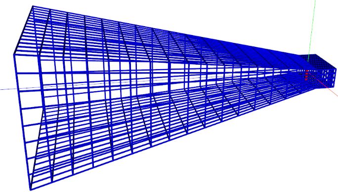
Preprints (www.preprints.org) | NOT PEER-REVIEWED | Posted: 6 June 2022                  doi:10.20944/preprints202206.0061.v1

                                                                                                                             2 of 36

                                 method) for solving a specific problem. According to [2], "the method is called optimal for
                                 solving a given class of problems with the required accuracy on a specified computing
                                 system if it allows you to get a result with minimal resource costs." Currently, there are
                                 many popular methods to solve electrodynamic problems numerically. The finite differ-
                                 ence method in the time domain (FDTD), was first described by K. Yee in 1966 [3], and the
                                 abbreviation of its name was proposed by A. Taflove [4]. The finite integration method
                                 (FIT) was proposed by T. Weiland in 1977 as a computational tool for solving Maxwell's
                                 equations [5]. The method can be implemented in both time and frequency domains.
                                 FDTD can be considered to be a special case of the FIT [6]. The finite element method
                                 (FEM) is widely used in the mechanical analysis of structures. Despite the fact that the
                                 mathematical interpretation of the method was proposed in 1943 by Courant [7], it was
                                 not used to solve electromagnetic problems until 1968. In general, these methods can solve
                                 problems of a complex structure and give accurate results. However, this happens at the
                                 expense of computational cost, especially when solving electrodynamic problems in the
                                 frequency domain, what will dramatically increase the costs to achieve the same required
                                 accuracy. The method of moments (MoM) seems to be most promising and more efficient
                                 for solving AE problems at relatively low computing costs. In relation to electrodynamic
                                 problems, the use of the MoM provides the following stages of solution. First, the metal
                                 parts of the studied AE are replaced by equivalent surface electric currents. Appropriate
                                 boundary conditions are imposed on the resulting solution of the metal elements to cal-
                                 culate the equivalent currents. Then, the problem of exciting the environment with these
                                 currents is solved. An important aspect of such process is the discretization of the metal
                                 surfaces into elementary areas and the approximation of the current within each such area.
                                       To approximate the curved boundaries of surfaces of an arbitrary shape, it is common
                                 to use the discretization into triangles, and to represent the current in them, using the
                                 vector basic functions RWG (Rao, Wilton, Glisson) [8]. This approach may be computa-
                                 tionally costly because of the time and memory required to build the numerical mesh and
                                 also the increase in the costs due to the need to solve a problem with the obtained big
                                 mesh. Moreover, the obtained mesh is not symmetrical, and it is sometimes hard to adjust
                                 it. Since the surface current in the symmetrical AE structures seems to distribute symmet-
                                 rically through the structure in a narrow frequency range, its more logical to get a sym-
                                 metrical mesh for a symmetrical structure. Therefore, this approach may not be efficient.
                                       As is known, the analysis of wire linear AEs is reduced to solving the integral Pock-
                                 lington [9] and Hallen [10] equations. The features of the solution of these equations are
                                 based on the thin-wire approximation [11–18]. In this approach, the wire is assumed to be
                                 an ideal conductor in the form of a cylinder located along one of the coordinate axes (a
                                 one-dimensional problem), with a radius much smaller than the wavelength of the exci-
                                 tation signal and the cylinder physical length. This simplification enables using a scalar
                                 current density function instead of a vector one, which greatly simplifies the complexity
                                 of the task. This approach is also applicable to the representation the AE surfaces by a
                                 wire-grid [19]. Such approach in combination with formulations of integral equations of
                                 the electric field and the MoM is widely used in well-known software products such as
                                 NEC [20]. Although, in comparison with the surface triangular approximation and the use
                                 of RWG functions, this approach demonstrates its inherent weaknesses in near-field anal-
                                 ysis, it has proven its efficiency on a large number of far-field scattering and radiation
                                 problems associated with conducting bodies of an arbitrary shape [21–25]. Therefore, the
                                 wire-grid approximation continues to be widely used in computational electrodynam-
                                 ics [26, 27], since it is very easy to adjust the obtained grid and it is more suitable for build-
                                 ing a symmetrical grid for symmetrical structures.
                                       There are many studies on summarizing and forming the criteria and conditions for
                                 the use of wire-grid surface approximation for AE modeling [19, 20, 23, 28–31]. In these
                                 sources, the proposed recommendations are not suitable for any AE structure and depend
                                 on the used weight and basics functions.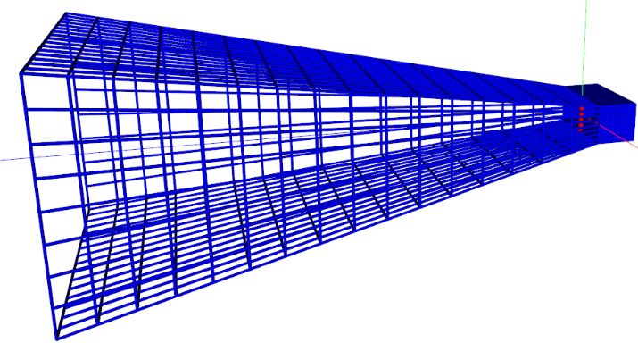
Preprints (www.preprints.org) | NOT PEER-REVIEWED | Posted: 6 June 2022               doi:10.20944/preprints202206.0061.v1

                                                                                                                         3 of 36

                                      This work is aimed to propose new recommendations for modeling symmetrical AE
                                 structures using the wire-grid surface approximation approach in combination
                                 with MoM.

                                 2. Materials and Methods
                                       None of the existing numerical methods is suitable for all electrodynamic modeling
                                 problems. Thus, MoM program codes are practically unsuitable for describing inhomoge-
                                 neous nonlinear dielectrics. FEM codes cannot effectively solve large scattering problems.
                                 Unfortunately, there are tasks where it is necessary to take into account all these features,
                                 for example, when evaluating radiation from a printed circuit board, and therefore, the
                                 analysis cannot be performed by any of these methods. One of the solutions to this prob-
                                 lem is to combine two or more methods in one program code. In this case, one of the
                                 methods is often MoM [32–39]. Each method is applied to the task field for which it is best
                                 suited. Appropriate boundary conditions are applied at the interfaces between these
                                 fields. Separately, it should be noted that the FDTD, FEM, and MoM are the most univer-
                                 sal methods and the largest number of books are devoted to their consideration where
                                 these methods are considered together, for example [1, 40–43]. The choice of a particular
                                 numerical method is based on the use of some criteria: the complexity of the geometry of
                                 the analyzed object; its electrical dimensions; available computing power; etc.
                                       Using MoM has an advantage since the modeled object can have a complex shape. In
                                 addition, MoM is most effective for open geometries with linear and homogeneous media.
                                 The method is excellent for hybridization with other methods and asymptotic procedures,
                                 for example, FMM and MLFMM (fast multipole method and multilevel fast multipole
                                 method), as well as UTD and GTD (homogeneous and geometric diffraction theory) [44].
                                 Unlike FEM and FDTD methods, MoM, when constructing the grid, does not require dis-
                                 cretization of the volume, in which the analyzed object is enclosed. It only requires dis-
                                 cretization of the surface of this object, which gives a relatively small cost for this proce-
                                 dure. Similarly to any other method, MOM has a disadvantages, in particular, it is difficult
                                 to model internal problems and heterogeneous media with this method. Besides, the cal-
                                 culation speed is sometimes low for objects of a relatively simple shape. However, this is
                                 easily eliminated by the speed increasing of workstations and developing of numerical
                                 procedures, which makes it possible to speed up the overall solution process using
                                 MoM [45].
                                       Based on the above, to solve antenna problems, it seems most effective to use the
                                 MoM, which is "surface" and not "volumetric" like the others, since its use does not require
                                 the boundary conditions that emulate remote boundaries to be artificially set. This reduces
                                 the dimension of the problem, reducing, for example, a three-dimensional problem to a
                                 two-dimensional one. In addition, the method allows for hybridization with other numer-
                                 ical methods. Therefore, if necessary, the functionality of the software module can be sig-
                                 nificantly expanded in the future. The computational aspects of MoM are considered in
                                 detail in [46–49].
                                       When using a particular numerical method, the important issue is related to its con-
                                 vergence rate and the accuracy of the results obtained with its help. Convergence when
                                 using MoM directly depends on the operator, the basis and test functions, as well as their
                                 number. At the same time, the effectiveness of using the method to obtain a result with a
                                 given accuracy is determined by the computational costs (the time and the memory of the
                                 workstation used). As a result, when calculating by the method of moments, an unknown
                                 quantity (for example, a field or current density) depending on spatial coordinates is ap-
                                 proximated by a finite number of known functions (called basis functions) multiplied by
                                 unknown coefficients. This approximation is substituted into a linear operator equation.
                                 The left and right sides of the resulting equation are multiplied by a suitable function
                                 (called a test or weight function) and integrated over the domain in which the test function
                                 is defined. Then the linear operator equation reduces to a system of linear algebraic equa-
                                 tion (SLAE). Repeating this procedure for a set of independent test functions, the number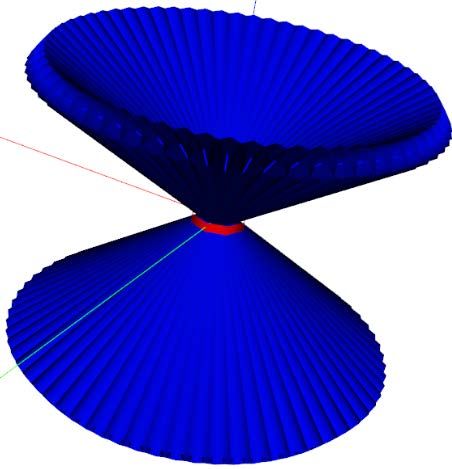
Preprints (www.preprints.org) | NOT PEER-REVIEWED | Posted: 6 June 2022                         doi:10.20944/preprints202206.0061.v1

                                                                                                                                   4 of 36

                                  of which should be equal to the number of basic functions, SLAEs are obtained. SLAEs
                                  solution gives unknown coefficients and allows finding an approximate solution to the
                                  operator equation. Further, the characteristics of interest are determined from the SLAEs
                                  solution.
                                        The MoM is widely applicable in modeling antennas of various classes. In addition,
                                  the method is most effective if the AE contains only perfectly conductive elements. In
                                  MoM, the choice of basic and test functions is determined by the shape of the entire con-
                                  ductive surface (structure). The most commonly used basic functions are called the piece-
                                  wise functions. They have a constant value in each meshing cell and equal to zero outside
                                  of it [50, 51]. One of the frequently used test functions that are not used as basic ones are
                                  Dirac delta functions (single impulse functions. When both piecewise and Dirac delta
                                  functions are employed, the MoM is known as the collocation method [52]. In addition,
                                  when similar basic and testing functions are employed, the MoM is known as the Galerkin
                                  method [47, 48].
                                        As mentioned above, an important aspect of using the MoM is the discretization of
                                  metal surfaces into elementary areas and the approximation of the current within each
                                  such area. Therefore, a summary of the recommendations for criteria and conditions, ex-
                                  tracted from various sources, can be formulated for the use of wire-grid surface approxi-
                                  mation in AE modeling [19, 20, 23, 28–31]:
                                  1.   The assumption of a thin wire must be fulfilled, i.e., the length of the wire L and the
                                       wavelength λ must be much larger than its radius a;
                                  2.   The wires of the grid should not intersect with each other along the length without
                                       forming a node (Figure 1). Hence, if two wires are electrically connected at their ends,
                                       then for current interpolation it is necessary to use the same coordinates to specify
                                       these ends;

                                                                        Wire1                                    Wire 1
            Wire 1                      Wire 1
                                                                                 Wire 2                 Wire 4            Wire 2
                     Wire 2                       Wire 2

                                                                        Wire 3                                   Wire 3            d
                              a                             b                               c

                                  Figure 1. Incorrect (a, b) and correct wire intersections (c, d)

                                  3.   Parallel wires should not be too close to each other. Hence, the distance between the
                                       axis of two (or more) wires connected in parallel should exceed their largest radius
                                       by more than 4 times;
                                  4.   The minimum number of basic functions for electrically shorted wires should be 3,
                                       especially if they are part of a wire-grid. For electrically short AEs, this number
                                       should be 8-10;
                                  5.   For an electrically short dipole, the number of segments (basic functions) must be at
                                       least 12-16;
                                  6.   For each individual wire, it is necessary to separately set the number of segments
                                       (basic functions) based on the frequency of the excitation signal (single calculation)
                                       or the highest frequency if the wire is modeled in the frequency range (multiple cal-
                                       culations). At the same time, it is not recommended to use less than 8-10 segments;
                                  7.   When setting the excitation at the intersection of the wires, an additional wire con-
                                       sisting of three segments is used. The source is set in the central part of this wire (Fig-
                                       ure 2). In this case, all segments in contact with the segment where the excitation
                                       source is located and near it must have the same length;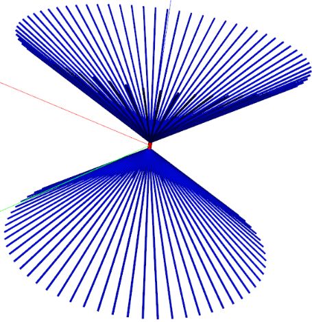
Preprints (www.preprints.org) | NOT PEER-REVIEWED | Posted: 6 June 2022                        doi:10.20944/preprints202206.0061.v1

                                                                                                                                       5 of 36

                     Node with an excitation sou rce                              Segment with an excitation source

                                                                                  Wire 4                          Wire 1
                  Wire 4                           Wire 1

                                                                                   Wire 3                   Wire 2
                  Wire 3                           Wire 2                               Wire 5 (3 segments)
                                                             a                                                                b

                                   Figure 2. Incorrect (a) and correct (b) setting of the excitation source at the wire intersection

                                   8.  In most cases, the length of the segments should be less than λ / 10, and when de-
                                       scribing complex geometric transitions – λ / 20. For large extended wire sections, the
                                       length of the segments can be increased, but it should not be less than λ / 5. At the
                                       same time, you should avoid using very short segments with a length of less than
                                       0.0001 λ;
                                   9. In most cases, the length of the segments should be more than 8–10 times their radius;
                                   10. In most cases, the appropriate wire-grid mesh is λ / 10 for the middle of the frequency
                                       range;
                                   11. The radius of the wire when using a wire-grid is determined through the surface area
                                       of the wires (the equivalent area rule). Thus, Figure 3 shows a grid element with a
                                       size of ∆ × ∆ formed by four wires, and the surface area of a wire with a diameter of
                                       2a. As a result, with a known grid step ∆, the required wire radius is defined as [53]

                                                                 a = ∆/2π.                                                                (1)

                    ∆                                                        ∆                      ∆

                               ∆         2a                                              2a                    2πa
                                               a                                                                      b

                                   Figure 3. A wire-gird element (a) and the area of one wire surface (b)

                                   12. If the wire-grid covers a surface having an irregular shape, then the equivalent area
                                       rule can be generalized as in [31]. Figure 4 shows an example of an approximation of
                                       a curved surface consisting of two regions A1 and A2. The required wire radius is
                                       calculated as

                                                         a = (A1+A2)/4∆π.                                                                 (2)

                                               ∆                      ∆      A1     A2
                                                            2a

                                   Figure 4. Modeling a curved surface with a single wire

                                        Using the above recommendations is not enough, and there are some problems oc-
                                   curring during the modeling process. In what follows, some cases will be presented in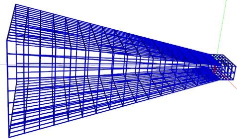
Preprints (www.preprints.org) | NOT PEER-REVIEWED | Posted: 6 June 2022                    doi:10.20944/preprints202206.0061.v1

                                                                                                                           6 of 36

                                 which considering the traditional recommendations for modeling symmetrical AE struc-
                                 tures using wire-grid approximation does not give correct results, and it is necessary to
                                 adjust these recommendations to get appropriate results. Moreover, some recommenda-
                                 tions will be presented for modeling such structures, and the results will be validated by
                                 comparing them with those obtained analytically and experimentally, as well as numeri-
                                 cally with another method. To do this and based on the wire-grid approximation and the
                                 MoM, a program module was developed using C++ programming language with
                                 OpenMP, VTK library, and the QT cross-platform software. This module (furtheron re-
                                 ferred to as the wire-grid) is used to calculate all the obtained results in this work. Besides,
                                 the Octave mathematical package was used to estimate the software implementation of
                                 the analytical models used later in this work to validate the results obtained using the
                                 wire-grid.

                                 3. Problems, solutions and results

                                 3.1. Modeling of a monopole on plate using wire-grid
                                       In the MoM, when wires are used to split the surfaces of the conductive parts in the
                                 structure into elementary platforms and approximate the current within them, a scalar
                                 current density function is used instead of a vector function, which greatly simplifies the
                                 solution. In this case, a preliminary choice of the number of the wires and their radius is
                                 required. The equal area rule is typically employed for constructing a square grid of wires
                                 when solving scattering problems [23, 26, 31, 54, 55]. However, the construction of such a
                                 grid is not always feasible, so it is necessary to use a different grid. Thus, we present a
                                 simple modification of the equal area rule for modeling structures using the wire-grid
                                 when solving the radiation problem.
                                       The known equal area rule is based on replacing a square polygon with a grid of
                                 wires, the radii of which are based on the size of the polygon [26]. The influence of the
                                 wire-grid size constructed considering this rule on the accuracy of the obtained results is
                                 investigated in [54]. The rule is generalized to the case of approximation of a surface con-
                                 sisting of square and triangular polygons [31]. The physical interpretation of the equal
                                 area rule is given in [55]. According to this rule, to approximate a square polygon with a
                                 separate wire, its radius a is determined so that the surface areas of the polygon and a wire
                                 length ∆ coincide as in (1) (see Figure 5a) [26].
                                       However, this rule cannot be applied in the case of a rectangular grid. In this case, it
                                 is proposed to use the length of the smaller side of the rectangle ∆2 (Figure 5b), i.e.
                                                            a = ∆2 / 2π.                                                      (3)

                                                           a                                     b
                                 Figure 5. Demonstration of the equal area rule [26] (a) and its modification (b)

                                       Testing was performed on the example of a dipole oriented along the x axis on a
                                 conducting plate 25×50 mm2 located in the yz plane. The dipole with a length of 12.5 mm
                                 (the length of its shoulders was 5, and the gap was 2.5 mm) and a radius of 0.015 mm was
                                 located at a distance of λ/4 from the end of the plate. The excitation frequency was
                                 7.56 GHz (λ≈39.655 mm). The wires with the radii calculated by (1) and (3) were modeled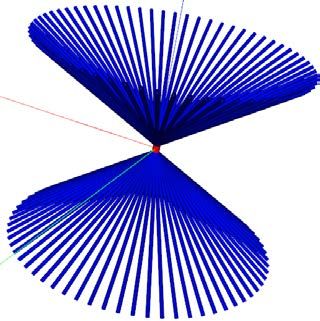
Preprints (www.preprints.org) | NOT PEER-REVIEWED | Posted: 6 June 2022                                     doi:10.20944/preprints202206.0061.v1

                                                                                                                                                          7 of 36

                                          using the wire-grid approximation. The EMPro (FDTD) system [56] was used for verifica-
                                          tion. The excitation port had the following characteristics: the amplitude of 1 V; the inter-
                                          nal resistance of 0 ohms; the signal form was "broadband". The segment length in both
                                          systems was assumed to be λ/10. Using the wire-grid approximation, the plate was ap-
                                          proximated by a grid Lу×Lz where Ly and Lz are the step numbers of the grid along the y
                                          and z axes. When a square grid was used, these values were assumed to be 8 and 4, re-
                                          spectively (the lengths of the wire segments on both axes were 6.25 mm). According to (1),
                                          the radius of the wires a =0.9947 mm was obtained. At λ/10, the length of the segments
                                          was 3.125 mm, which satisfies the conditions in the recommendation 1 and 10 (later will
                                          be referred to as conditions (1, 10) ). As a result, each piece of wire was divided into 2
                                          segments. The total number of segments N was 157. When a rectangular grid was used,
                                          Lу=Lz=8 was assumed (the lengths of the wire segments along the y and z axes were 6.25
                                          and 3.125 mm). The radius of the wires according to (3) was 0.5 mm, and the length of the
                                          segments was 3.125 mm, which also satisfies the conditions (1, 10). The wire segments
                                          along the y axis were divided into 2 segments, and z were not divided and the value of N
                                          was 221. The obtained radiation patterns (RP) are shown in Figure 6, and at θ=0, 1, ..., 180,
                                          ϕ = 0°, 45° and 90° – in Figure 7.

                                          a                                                 b                                                  c

                                          Figure 6.The RP of a dipole on a conducting plate modeled using the wire-grid
                                          by (1) (a), by (3) (b) and EMPro (c)

                             |E|, V/m                                          |E|, V/m                                           |E|, V/m
                         0                                                 0                                                  0
                   345          15                                   345         15                                     345           15
             330                    30                         330                     30                         330                     30
          315                            45                 315                             45                 315                             45
        300                                   60          300                                    60          300                                    60
       285                                     75        285                                      75        285                                      75
      270                                      90        270                                      90        270                                      90
       255                                     105       255                                      105       255                                      105
        240                               120             240                               120              240                                120
          225                           135 θ, °            225                           135 θ, °             225                            135 θ, °
             210                     150                       210                     150                        210                      150
                   195 180     165                                   195 180     165                                    195 180      165

                                                     a                                                  b                                                      c
                                          Figure 7. The RP of a dipole on a conducting plate at θ = 0, 1, ..., 180°, ϕ = 0° (a), 45° (b) and 90° (c)
                                          using the wire-grid by (1) (––), by (3) (----), and EMPro (⋅⋅⋅⋅)

                                               From Figures 6 and 7 it can be seen that the results of EMPro and with the wire-grid
                                          by (3) agree very well, and the maximum of the electric field strength magnitudes |E| are
Preprints (www.preprints.org) | NOT PEER-REVIEWED | Posted: 6 June 2022 doi:10.20944/preprints202206.0061.v1
8 of 36
very close: 0.479 and 0.475 V/m (the difference is less than 1%). When using (1), the maxi-
mum |E| was 0.548 V/m (13% difference from EMPro). Thus, one can say that the pro-
posed rule (3) gives more accurate results compared to (1).
3.2. Modeling symmetrical biconical AEs
When modeling a complex structure, like a symmetrical biconical AE presented in
(Figure 8), it is inappropriate to use the traditional recommendations for modeling. The
number of wires and their radii are difficult to determine, as well as the radius of the wire
where the excitation source is located. Moreover, to answer the questions about wire lo-
cation in the grid (horizontal and vertical grid elements) and the effect of the segment step
on the results is not a trivial issue here. Therefore, the following model-testing based on
wire-grid approximation model was performed in order to reveal an optimal setting for
modeling such AE structure.
φ θ
Θ1
h
φ θ a
Θ0
g
a h
g
Ground plane Coaxial line
Θ2
a b
Figure 8. The conical (a) and the biconical (b) AEs
When the wire-grid approximation was employed based on the convergence of the
results obtained by increasing the number of wires (4, 8, 16, 32, 64, and 128) approximating
the AE surface, it was found that their optimal number is 64. The horizontal grid elements
were not used here because the amplitudes of the distributed currents among them are
very small and their contribution to the radiated electric field is negligible. The values of
the length of the segment ls, the radius of the structure wires as and the radius of the wire
in the gap (excitation source) agap, were determined as ls = λ / n, as = ls / 10, agap = ls / 5, re-
spectively. The wire in the gap was approximated by one segment. A general view of the
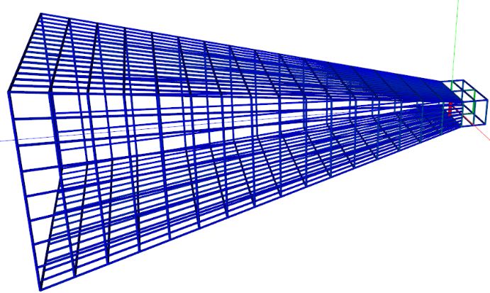
biconical AE at specified frequencies is shown in Figure 9.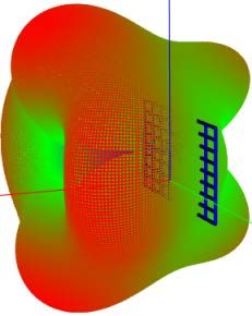
Preprints (www.preprints.org) | NOT PEER-REVIEWED | Posted: 6 June 2022                doi:10.20944/preprints202206.0061.v1

                                                                                                                          9 of 36

                                      Calculations of the radiotechnical characteristics (RTC) of the biconical AE were per-
                                 formed using the wire-grid, as well as the EMPro at frequencies of 0.1, 0.5, and 1 GHz
                                 with a gap length of 20 mm. The obtained results are compared to each other and to those
                                 obtained using well–known analytical expressions [57–59] (see Appendix A) to verify
                                 them and to prove that the proposed recommendations can give accurate results with low
                                 computational costs.
                                      In general, the resulting inaccurate solution is not necessarily related to the used com-
                                 putational algorithm of the numerical method that was employed; it may be related to the
                                 solved mathematical problem itself. Even with an accurate calculation, the solution of the
                                 problem can be very sensitive to the disturbances in the input data. The qualitative con-
                                 cept of this sensitivity and its quantitative measure, which is called conditionality, are
                                 related to the influence of the disturbances in the input data on the resulting solution.
                                 Therefore, a problem is called insensitive or well-conditioned if this relative change in the
                                 input data causes a reasonably commensurate relative change in the solution. On the con-
                                 trary, task is considered sensitive or poorly conditioned if the relative change in the solu-
                                 tion can be much greater than it is in the input data. For quantitative evaluation, the con-
                                 dition number of the problem is used in the form of the ratio of the relative change in the
                                 solution to the relative change in the input data. Then, the task is poorly conditioned or
                                 sensitive if its condition number is much greater than one. Otherwise, the task is consid-
                                 ered well-conditioned.
                                      Since the MoM reduces the surface integral equation of the electric field to a SLAE,
                                 which integrally contains all the information about the object under study, the properties
                                 of the obtained SLAE have to be analyzed in order to assess the stability of the problem
                                 solution; in the case under consideration – RTC AE. Therefore, when using MoM, many
                                 elements of matrix Z and of vectors V are obtained by numerical integration. Conse-
                                 quently, small errors in integration can be "increased" by a poorly conditioned Z matrix.
                                 In general, it is customary to evaluate the measure of conditionality of a matrix using its
                                 condition number [60]
                                                 cond(Z)=|| Z|| ||Z-1||                                                    (4)
                                 where || ⋅ || is a certain matrix norm. Conditionality characterizes the sensitivity of the
                                 SLAE solution to the changes in the values of the matrix elements. The higher the condi-
                                 tion number of the matrix, the worse it is conditioned (for a single element matrix it is
                                 equal to 1). As the condition number of increases, the error of the solution increases be-
                                 cause floating-point numbers are represented by a finite number of digits [61]. One of the
                                 important consequences of this is that a correct solution of SLAE cannot be obtained by
                                 the Gauss method with a small bit representation of numbers because of the large condi-
                                 tion number of matrix Z [62]. As a result, the required numerical accuracy of the calculated
                                 result must exceed the probable number of the lost digits since the errors are rounded
                                 during calculations. This number of digits can be estimated by the conditionality number
                                 of the matrix. So, basically, if cond(Z) = O(10p) and the source data have an error in the kth
                                 decimal point, then regardless of the used method for solving the SLAE equation ZI = V,
                                 it is guaranteed to get its solution with no more than k – p decimal points [63].
                                       For example, suppose that when the convergence of a solution is investigated by in-
                                 creasing the number of basic functions, the condition number of matrix Z is of the order
                                 of 106. Then, if it is necessary that the results for the input impedance converge to the fifth
                                 decimal point, then the elements of the matrix Z must be calculated with an accuracy of
                                 at least 11 digits, and this number of digits must be preserved in all calculations [63]. Re-
                                 member that the condition number does not give an exact value of the maximum error of
                                 the method used, but only allows estimating its order. Therefore, you can specify an upper
                                 bound for the condition number, if it is exceeded, the solution of the SLAE at a particular
                                 workstation will lead to false results. Thus, if

                                                     cond(Z)≥ 1/eps                                                          (5)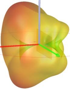
Preprints (www.preprints.org) | NOT PEER-REVIEWED | Posted: 6 June 2022                     doi:10.20944/preprints202206.0061.v1

                                                                                                                                 10 of 36

                                 where eps is the machine epsilon, then the solution is considered unreliable [61, 63, 64].
                                       According to IEEE 754–2008, for calculations with single and double precision, the
                                 eps value is O(10–7) and O(10–16), respectively. Often, when solving large-scale problems,
                                 even the conditionality number of matrix Z is large, but it is less than 1 / eps, so the MoM
                                 is workable [65]. However, the conditionality of the SLAE matrix worsens when the exci-
                                 tation frequency approaches the frequencies of natural oscillations (internal resonances)
                                 of the structure under study, especially at low frequencies [65]. Since the excitation fre-
                                 quency is selected discretely, there is a possibility of such a coincidence. The solution at
                                 this frequency may not be obtained at all, and at close frequencies it may be inaccurate or
                                 completely incorrect. For example, [66–70] are devoted to demonstrating the presence of
                                 imaginary resonances that do not exist in reality. To avoid this, it’s necessary to increase
                                 the bit depth of the number representation [71] or to use the iterative methods [62, 72].
                                       The influence of the mesh step (segments), set as λ / n, on the accuracy of the calcu-
                                 lated RTC of AEs at n = 10, 20, and 40 was studied. The required orders of the formed
                                 matrices Z of the SLAE and their condition number (cond) calculated by (4) when using
                                 the wire-grid are summarized in Table 1.
                                       The values of the input impedance of the biconical AE obtained using the wire-grid
                                 and the EMPro (FDTD) system, are summarized in Table 2. The table shows that the re-
                                 sults obtained in the developed wire-grid software, as well as the EMPro (FDTD) system,
                                 converge when the grid step decreases. Table 4 shows the deviations of the input imped-
                                 ance magnitude values obtained in EMPro and using the wire-grid, relative to those ob-
                                 tained by analytical expressions. It can be seen that reducing the grid step gives values
                                 closer to the analytical ones, and using the wire-grid approximation gives closer results to
                                 the analytical ones from EMPro with less computational costs. In the EMPro system at
                                 n = 40, no results were obtained, due to machine memory limitations, so they are not listed
                                 in the tables (marked as «–»). The elapsed simulation time (T) and the used memory (M)
                                 for simulating the RTC of the of the biconical AE using the wire-grid and EMPro, are pre-
                                 sented in Table 4 and Table 5, respectively.

                                        a                                              b                                            c

                                 Figure 9. A general view of the biconical AE at frequencies of 0.1 (a), 0.5 (b), and 1 GHz (c) (the view
                                 is changing because the wire radius reduces with the frequency growth)
Preprints (www.preprints.org) | NOT PEER-REVIEWED | Posted: 6 June 2022 doi:10.20944/preprints202206.0061.v1
11 of 36
Table 1. The matrix Z orders N and their condition numbers, for the biconical AE with a = 508 mm
and Θ1 = Θ2 = 53.1°at frequencies of 0.1, 0.2 and 1 GHz and mesh step (segment size) λ / n
Frequency (GHz) n N cond
10 257 1.4*105
0.1 20 513 2.2*106
40 897 3.1*105
10 1153 2.7*105
0.5 20 2177 5.7*105
40 4353 9.6*106
10 2177 8.2*104
1 20 4353 1.6*105
40 8705 6.4*105Preprints (www.preprints.org) | NOT PEER-REVIEWED | Posted: 6 June 2022 doi:10.20944/preprints202206.0061.v1
12 of 36
Table 2. The input impedance values for the biconical AE with a = 508 mm and Θ1 = Θ2 = 53.1°
at frequencies of 0.1, 0.2, and 1 GHz and a mesh step (segment size) λ / n
Frequency (GHz) n (A1), (A11) EMPro Wire-grid
10 29.73 + j15.78 0.46 – j25.48
0.1 20 40.40 + j28.32 39.51 + j12.95 192.31 – j58.89
40 – 28.01 + j25.59
10 117.48 + j64.27 114.01 – j6.29
0.5 20 101.80 – j9.38 112.89 + j74.69 102.02 + j33.36
40 – 90.44 + j48.18
10 116.40 + j89.92 103.11 + j41.34
1 20 88.64 + j16.68 117.84 + j112.36 88.29 + j56.82
40 – 84.62 + j71.55
Table 3. The deviation (%) of the input impedance magnitudes from Table 2 calculated using
the wire-grid and EMPro comparing to those obtained analytically
Frequency (GHz) n EMPro Wire-grid
10 31.78 48.35
0.1 20 15.73 307.65
40 – 23.10
10 30.99 11.69
0.5 20 32.41 4.99
40 – 0.23
10 63.08 23.16
1 20 80.52 16.41
40 – 22.86
Table 4. The elapsed time and used memory for simulating the biconical AE using the wire-grid,
with a = 508 mm and Θ1 = Θ2 = 53.1°
at frequencies of 0.1, 0.2, and 1 GHz and a mesh step (segment size) λ / n
Frequency (GHz) n T (s) M (MB)
10 0.34 1
0.1 20 0.51 4
40 0.60 12.28
10 1.02 20.29
0.5 20 4.11 72.31
40 19.29 289.13
10 4.03 72.31
1 20 18.29 289.13
40 109.06 1156.27Preprints (www.preprints.org) | NOT PEER-REVIEWED | Posted: 6 June 2022 doi:10.20944/preprints202206.0061.v1
13 of 36
Table 5. The elapsed time to obtain the RTC at each frequency, the total simulation time (Tt) and the
used memory for simulating the biconical AE using EMPro, with a = 508 mm and Θ1 = Θ2 = 53.1°at
frequencies of 0.1, 0.2, and 1 GHz and a mesh step (segment size) λ / n.
Frequency Physical/virtual Required Problem
n T (s) Tt (s)
(GHz) memory (MB) (GB) size (cells)
0.1 159
10 0.5 181 921 903/922 1.2 331*311*245
1 183
0.1 567
20 0.5 649 1892 4722/4753 6 584*581*448
1 676
0.1 – –
40 0.5 – – – 36 1126*1120*855
1 – –
Figures 10–12 show the RP obtained using the wire-grid with decreasing mesh size
(segments number) at frequencies of 0.1, 0.2 and 1 GHz, respectively. Additionally, for
clarity, similar results obtained in EMPro are given.
0 |E|N
345 15
330 30
315 45 wire-grid, λ/10
300 60
wire-grid, λ/20
285 75
270 90 wire-grid, λ/40
255 105
EMPro, λ/10
240 120
225 135 EMPro, λ/20
210 150 θ,°
195 165
180
Figure 10. The normalized RP (|E|N, times) of the biconical AE with a = 508 mm and Θ1 = Θ2 = 53.1°
when ka1 = 1.0640 (f1 = 0.1 GHz), calculated by the wire-grid and EMProPreprints (www.preprints.org) | NOT PEER-REVIEWED | Posted: 6 June 2022 doi:10.20944/preprints202206.0061.v1
14 of 36
0 |E|N
15 15
30 30
45 45 wire-grid, λ/10
60 60
wire-grid, λ/20
75 75
90 90 wire-grid, λ/40
105 105
EMPro, λ/10
120 120
135 135 EMPro, λ/20
150 150 θ,°
165 165
180
Figure 11. The normalized RP (|E|N, times) of the biconical AE with a = 508 mm and Θ1 = Θ2 = 53.1°
when ka2 = 5.3198 (f1 = 0.5 GHz), calculated by the wire-grid and EMPro
0 |E|N
345 15
330 30
315 45 wire-grid, λ/10
300 60
wire-grid, λ/20
285 75
270 90 wire-grid, λ/40
255 105
EMPro, λ/10
240 120
225 135 EMPro, λ/20
210 150
195 165 θ,°
180
Figure 12. The normalized RP (|E|N, times) of the biconical AE with a = 508 mm and Θ1 = Θ2 = 53.1°
when ka3 = 10.6395 (f1 = 1 GHz), calculated by the wire-grid and EMPro
In figures 16–18 the results obtained by using the wire-grid, the EMPro (FDTD) sys-
tem (λ/10 mesh was used in the further comparisons since it’s results seem to be closer to
the analytical ones), and the analytical expressions are summarized. In general, all the
results are consistent with each other. Table 6 shows the largest differences in the calcu-
lated values compared to those obtained by(A8).Preprints (www.preprints.org) | NOT PEER-REVIEWED | Posted: 6 June 2022 doi:10.20944/preprints202206.0061.v1
15 of 36
0 |E|N
345 15
330 30
315 45 [58]
300 60
(A8)
285 75
270 90 (A9)
255 105
wire-grid, λ/40
240 120
225 135 EMPro, λ/10
210 150 θ, °
195 165
180
Figure 13. The normalized RP (|E|N, times) of the biconical AE when ka1 = 1.0640 (f1 = 0.1 GHz),
calculated analytically and by the wire-grid and EMPro at different mesh sizes
0 |E|N
345 15
330 30
315 45 [58]
300 60
(A8)
285 75
270 90 (A9)
255 105
wire-grid, λ/40
240 120
225 135 EMPro, λ/10
210 150 θ, °
195 165
180
Figure 14. The normalized RP (|E|N, times) of the biconical AE when ka2 = 5.3198 (f1 = 0.5 GHz),
calculated analytically and by the wire-grid and EMPro at different mesh sizesPreprints (www.preprints.org) | NOT PEER-REVIEWED | Posted: 6 June 2022 doi:10.20944/preprints202206.0061.v1
16 of 36
0 |E|N
345 15
330 30
315 45 [58]
300 60
(A8)
285 75
270 90 (A9)
255 105
wire-grid, λ/40
240 120
225 135 EMPro, λ/10
210 150 θ, °
195 165
180
Figure 15. The normalized RP (|E|N, times) of the biconical AE when ka3 = 10.6395 (f1 = 1 GHz),
calculated analytically and by the wire-grid and EMPro at different mesh sizes
Table 6. The maximum differences of normalized RP values obtained at different mesh sizes λ / n
and by (A8) at frequencies of 0.1, 0.2, and 1 GHz
Frequency (GHz) n EMPro Wire-grid
10 0.0189 0.0259
0.1 20 0.0189 0.0236
40 – 0.0211
10 0.1080 0.1869
0.5 20 0.1030 0.1395
40 – 0.1395
10 0.1291 0.1569
1 20 0.1268 0.1197
40 – 0.1669
As can be seen from Table 2–6 and Figures 10–18, the estimated RTC AE results and
their calculation error using the wire-grid were compared to those obtained analytically
and using the EMPro system. It is shown how the decrease in the grid step affects the
obtained values of the RP and the input impedance. The RPs obtained using the wire-grid
are close to those obtained using the analytical expressions. At the same time, the compu-
tational costs when using the wire-grid are much less than those obtained using
the EMPro system. The obtained results proved that using the proposed recommenda-
tions for modeling the symmetrical biconical AE can give accurate results and with less
computational costs.
3.3. Modeling horn AE
Another complex structure to be modeled is a horn AE presented in (Figure 16). The
cross section of this AE is symmetrical in two planes. This AE is also simulated and tested
using the wire-grid approximation, and new recommendations for modeling it are deter-
mined and provided further. The inner surface geometrical parameters of this AE are pre-
sented in Table 7. The wall thickness of the regular part of the AE is 1 mm, and the irreg-
ular part is 2 mm. For verifying the obtained results of modeling the horn RTCs, the re-
sults are compared with the measured ones for a manufactured prototype of this horn (its
parameters after manufacturing are measured and also presented in Table 7). The AE wasPreprints (www.preprints.org) | NOT PEER-REVIEWED | Posted: 6 June 2022 doi:10.20944/preprints202206.0061.v1
17 of 36
modeled using the wire-grid at an operating frequency of 8 GHz. The AE was excited by
installing a wire at the junction of the regular and irregular parts of the horn between its
wide walls. The length of the wire corresponded to the value b from Table 7. The wire was
approximated by one segment. After performing model-testing based on the wire-grid
approximation model, the following recommendations were obtained for modeling these
types of AEs.
For common issues, a wide range of parameters was used. The RTCs of the AE were
calculated with a decrease in the mesh step of the grid λ / n and an increase in the number
of wires to approximate the surface of the regular part of the AE. When modeling, the
wide walls of the regular part (the index r is used to denote the regular part of the AE)
were divided into SZr parts along the z axis and SXr parts along the x axis, the narrow
sides were SZr and SYr, and the back shortened wall was divided into SXr and SYr, respec-
tively. The ratios SZr = SXr = Lr, SYr = Lr / 2 were used. To approximate the extended part
of horn (the index e is used to denote the extended part of the AE) its wide walls were
divided into SZe parts on the z axis and SXe parts along the x axis, and narrow ones – SYe
parts along the y axis. It is assumed that SYe = SXe / 2 and the ratios SZe = SXe = Le,
SYe = Le / 2 were used. The order N of the SLAE matrix Z with using the values of n = 10, 20,
40, Le = 16 for the irregular part of the horn AE, and Lr = 2, 4, 8, 16 for the regular part, are
given in Table 8. Moreover, the condition numbers for matrix Z are presented along with
the time consumed to calculate them, as well as the total numbers of wire used to model
the regular and the extended parts of the AE. General views of the AE with the Lr values
are shown in Figure 17. The values Le = 16 and Lr = 8 seem to be minimal optimal values
(see Appendix B) for modeling such AEs. The calculated values of the normalized magni-
tude of the electric field strength (|E|N, dB) at ϕ = 0° и ϕ = 90° are shown in Figure 18, and
demonstrate convergence with an increase of n. Therefore, the value n = 40 seems to be
optimal. The values of the segment length ls, the radius of the structure wires as and the
radius of the wire where the excitation was applied aex, were determined as ls = λ / n,
as = ls / 10, aex = ls / 5, respectively. The wire where the excitation was applied was approx-
imated by one segment.
ap
y
φ θ
x z
a bp
br
b
ar lr
l
Figure 16. The isometric view of the inner surface of the horn AE
Table 7. The geometrical parameters (mm) of the inner surface of the horn AE
Geometrical
ap bp a b ar br l lr
parameter
Model 80 60 23 10 23 10 150 10
Prototype 79.9 59.8 23.0 10.0 23.0 10.0 149.9 10.0Preprints (www.preprints.org) | NOT PEER-REVIEWED | Posted: 6 June 2022 doi:10.20944/preprints202206.0061.v1
18 of 36
a b
c d
Figure 17. General views of AEs with the wire used as an excitation source built in the wire-grid
using Le = 16 and Lr = 2 (a), 4 (b), 8 (c), and 16 (d)
Table 8. Total wire number (TWN) and the order N of the SLAE matrix Z for the horn AE at different
mesh step of the grid λ / n using the wire-grid and Le = 16, and Lr = 2, 4, 8, 16; the condition number
for matrix Z (cond) and the time consumed to calculate Z (T).
n
Lr TWN 10 20 40
N T (s) cond N T (s) cond N T (s) cond
2 1609 3544 1.65 2.35*104 5931 4.40 8.68*104 11448 16.80 3.76*105
4 1687 3636 1.71 2.41*104 6112 4.73 8.91*104 11742 17.46 1.89*106
8 1999 3906 2.01 3.28*104 6480 5.25 1.02*105 12464 19.25 4.48*105
16 3247 5178 3.44 3.69*105 7556 7.10 2.07*106 13936 24.49 9.81*105
0 |E|N, dB 10 0 |E|N, dB 10
345 15 20 345 15 20
330 30 330 30 40
315 45 40 315 45
300 60 300 60
285 75 285 75
270 90 270 90
255 105 255 105
240 120 240 120
225 135 225 135
θ, °
210 150 210 150 θ, °
195 165 195 165
180 a 180 b
Figure 18. The RPs (|E|N, dB) of the horn AE at the frequency of 8 GHz in the φ = 90° (a)
and φ = 0° (b) planes in the wire-grid with Le = 16 and Lr = 8, n = 10, 20, 40Preprints (www.preprints.org) | NOT PEER-REVIEWED | Posted: 6 June 2022 doi:10.20944/preprints202206.0061.v1
19 of 36
The prototype of the horn AE with the parameters presented in Table 7 was manu-
factured, and its RTCs were measured in order to validate the results calculated using the
wire-grid approximation. Figure 19 compares the results of the normalized RPs obtained
using the wire-grid (Lr = 8, SXe = SZe = 16) and experimentally at ϕ = 0° and ϕ = 90°. Table 9
summarizes the calculated and the measured AE main beamwidths (BW) and the levels
of the sidelobes (SLmax).
Table 9. The calculated and measured RTCs of the horn AE
RTC Wire-grid Measured
BW (°), φ = 90° 25 31
BW (°), φ = 0° 34 31
SLmax (dB) –12.61 -16.93
0 |E|N, dB 0 |E|N, dB
345 15 345 15
330 30 330 30
315 45 315 45
300 60 300 60
285 75 285 75
270 90 270 90
255 105 255 105
240 120 240 120
225 135 θ,° 225 135
θ,°
210 150 210 150
195 165 195 165
180 a 180 b
Figure 19. The measured () and the calculated (⋅⋅⋅⋅) RPs (|E|N, dB) of the horn AE at the frequency
of 8 GHz in the φ = 90° (a) and φ = 0° (b) planes in the wire-grid with Le = 16 and Lr = 8, n = 40. The
level of –3 dB (---).
Then we compared the results of simulation with the changing of the grid to the
measured results. Figures 20–22 show the RPs for the horn AE using Lr = 8, 16, 32 and
Le = 16, 32 and SZe = SXe or equal to SXe*2±1. Figure 23 summarizes these results together
for clarity and the numbers in the graphics legend refer to Lr, SXe, SZe, respectively. As can
be seen from Figures 20–23, if the grid cells are refined to have a closer to square shape,
the obtained results can be closer to the measured ones. Note that the results using the
same value for SZe are very close except at the back lobe where the denser grid gives less
radiation level. Therefore, one can say that the optimal grid form is symmetrical, denser,
and squarer. This corresponds to SZe = SXe=32. Figure 24 compares the results considering
this point. It can be seen that the results are almost identical and increasing the density of
the grid will not produce more accurate results, but will only increase the computational
costs as can be seen from Table 10 in which the calculated condition numbers and the
input impedance (Z=R+jX) of the horn AE and the time consumed to calculate them at
different mesh and grid settings using wire-grid approximation are presented.Preprints (www.preprints.org) | NOT PEER-REVIEWED | Posted: 6 June 2022 doi:10.20944/preprints202206.0061.v1
20 of 36
0 |E|N, dB 8_16_16 0 |E|N, dB 8_16_16
345 15 345 15
330 30 8_16_32 330 30 8_16_32
315 45 8_32_16 315 45 8_32_16
300 60 8_32_32 300 60 8_32_32
285 75 measured 285 75 measured
minus 3 dB minus 3 dB
270 90 270 90
255 105 255 105
240 120 240 120
225 135 θ,° 225 135 θ,°
210 150 210 150
195 165 195 165
180 a 180 b
Figure 20. The measured and the calculated RPs (|E|N, dB) of the horn AE at the frequency of 8 GHz
in the φ = 90° (a) and φ = 0° (b) planes in the wire-grid with Lr = 8, n = 40, Le = 16, 32 and SZe = SXe or
equal to SXe*2±1. The level of –3 dB (---).
0 |E|N, dB 16_16_16 0 |E|N, dB 16_16_16
345 15 345 15
330 30 16_16_32 330 30 16_16_32
315 45 16_32_16 315 45 16_32_16
300 60 16_32_32 300 60 16_32_32
measured measured
285 75 285 75
minus 3 dB minus 3 dB
270 90 270 90
255 105 255 105
240 120 240 120
225 135 θ,° 225 135 θ,°
210 150 210 150
195 165 195 165
180 a 180 b
Figure 21. The measured and the calculated RPs (|E|N, dB) of the horn AE at the frequency of 8 GHz
in the φ = 90° (a) and φ = 0° (b) planes in the wire-grid with Lr = 16, n = 40, Le = 16, 32 and SZe = SXe
or equal to SXe*2±1. The level of –3 dB (---).
0 |E|N, dB 32_16_16 0 |E|N, dB 32_16_16
345 15 345 15
330 30 32_16_32 330 30 32_16_32
315 45 32_32_16 315 45 32_32_16
300 60 32_32_32 300 60 32_32_32
measured measured
285 75 285 75
minus 3 dB minus 3 dB
270 90 270 90
255 105 255 105
240 120 240 120
225 135 θ,° 225 135 θ,°
210 150 210 150
195 165 195 165
180 a 180 b
Figure 22. The measured and the calculated RPs (|E|N, dB) of the horn AE at the frequency of 8 GHz
in the φ = 90° (a) and φ = 0° (b) planes in the wire-grid with Lr = 32, n = 40, Le = 16, 32 and SZe = SXe
or equal to SXe*2±1. The level of –3 dB (---).Preprints (www.preprints.org) | NOT PEER-REVIEWED | Posted: 6 June 2022 doi:10.20944/preprints202206.0061.v1
21 of 36
|E|N, dB 8_16_16 0 |E|N, dB 8_16_16
0
345 15 8_16_32 345 15 8_16_32
330 30 330 30
8_32_16 8_32_16
315 45 315 45
8_32_32 8_32_32
300 60 16_16_16 300 60 16_16_16
285 75 16_16_32 285 75 16_16_32
16_32_16 16_32_16
270 90 16_32_32 270 90 16_32_32
32_16_16 32_16_16
255 105 255 105
32_16_32 32_16_32
240 120 32_32_16 240 120 32_32_16
225 135 θ,° 32_32_32 225 135 θ,° 32_32_32
210 150 measured 210 150 measured
195 165 minus 3 dB 195 165
180 a 180 minus 3 dB b
Figure 23. The measured and the calculated RPs (|E|N, dB) of the horn AE at the frequency of 8 GHz
in the φ = 90° (a) and φ = 0° (b) planes in the wire-grid with Lr = 8, 16, 32, n = 40, Le = 16, 32 and
SZe = SXe or equal to SXe*2±1. The level of –3 dB (---).
0 |E|N, dB 8_32_32 0 |E|N, dB 8_32_32
345 15 345 15
330 30 16_32_32 330 30 16_32_32
315 45 315 45
32_32_32 32_32_32
300 60 300 60
measured measured
285 75 285 75
minus 3 dB minus 3 dB
270 90 270 90
255 105 255 105
240 120 240 120
225 135 θ,° 225 135 θ,°
210 150 210 150
195 165 195 165
180 a 180 b
Figure 24. The measured and the calculated RPs (|E|N, dB) of the horn AE at the frequency of 8 GHz
in the φ = 90° (a) and φ = 0° (b) planes in the wire-grid with Lr = 8, 16, 32, n = 40, Le = 32 and SZe = SXe.
The level of –3 dB (---).Lr
|Z| (Ohm) X (Ohm) R (Ohm) cond T (s) N TWN SZe SXe
349.05 267.54 227.18 3.28*104 6.42 3906 1584+415 16
16
405.37 274.63 298.17 5.02*104 15.12 5794 3120+415 32
8
353.76 267.14 231.90 7.37*104 21.60 6674 3168+415 16
32
419.12 288.83 303.70 1.50*105 52.72 9746 6240+415 32
350.73 275.49 217.05 3.69*105 12.43 5178 1584+1663 16
16
408.76 290.37 287.70 4.50*105 24.05 7066 3120+1663 32
16
355.34 275.55 224.36 4.72*105 31.47 7946 3168+1663 16 10
32
420.98 304.27 290.93 6.05*105 64.34 11018 6240+1663 32
352.16 277.11 217.33 2.75*107 54.28 10218 1584+6655 16
410.44 292.70 287.74 3.12*107 83.22 12106 3120+6655 32 16
settings
32
354.92 276.17 222.93 5.10*107 97.87 12986 3168+6655 16
32
167.24 305.65 289.09 5.91*107 167.24 16058 6240+6655 32
4. Conclusions
394.50 330.36 215.68 1.03*105 19.10 6480 1584+415 16
16
411.94 306.99 274.68 1.26*105 41.30 9120 3120+415 32
8
396.95 326.06 226.40 1.80*105 61.06 10688 3168+415 16
32
435.17 321.58 293.19 2.60*105 131.29 14464 6240+415 32
398.26 341.40 205.07 2.07*106 27.56 7556 1584+1663 16
16
421.83 328.61 264.48 2.49*106 55.39 10196 3120+1663 32
n
16
20
402.63 339.68 216.17 2.56*106 77.57 11764 3168+1663 16
32
ing the required modeling accuracy.
445.14 346.79 279.08 3.15*106 157.34 15540 6240+1663 32
Preprints (www.preprints.org) | NOT PEER-REVIEWED | Posted: 6 June 2022
401.79 345.87 204.48 5.28*106 92.08 12644 1584+6655 16
16
427.13 335.80 263.96 5.80*106 154.39 15284 3120+6655 32
32
403.93 342.88 2113.53 5.96*106 186.79 16852 3168+6655 16
32
447.57 352.96 275.19 6.77*106 311.35 20628 6240+6655 32
452.75 400.66 210.86 4.48*105 90.19 12464 1584+415 16
16
439.20 366.40 242.17 4.58*105 161.69 15792 3120+415 32
8
448.43 389.78 221.74 8.76*105 311.84 20544 3168+415 16
32
460.08 368.76 275.12 7.89*105 473.22 24288 6240+415 32
460.55 415.03 199.63 9.81*105 121.86 13936 1584+1663 16
16
453.40 388.28 234.12 1.07*106 202.88 17264 3120+1663 32
40
16
459.54 407.21 212.97 1.40*106 372.68 22016 3168+1663 16
32
479.79 399.02 266.42 1.44*106 542.52 25760 6240+1663 32
461.96 419.44 193.60 2.94*106 219.29 18232 1584+6655 16
16
457.11 395.82 228.65 3.15*106 352.75 21560 3120+6655 32
32
462.38 413.16 207.58 3.50*106 570.93 26312 3168+6655 16
32
doi:10.20944/preprints202206.0061.v1
485.20 409.90 259.63 3.72*106 851.60 30056 6240+6655
visable to search for other ways to save machine computational resources while maintain-
32
effective computational approach for modeling symmetrical AEs with low computational
In this paper we focused on the use of the MoM and wire-grid approximation as an
widely used nowadays. The use of this method leads to reducing the integral equation to
cost and quite accurate results. For AE modeling, the MoM using RWG basic functions is
SLAE, the order of which determines the required machine memory. Therefore, it is ad-
22 of 36
Table 10. The calculated RTCs of the horn AE using the wire-grid with different mesh and gridPreprints (www.preprints.org) | NOT PEER-REVIEWED | Posted: 6 June 2022 doi:10.20944/preprints202206.0061.v1
23 of 36
One such approach is the wire-grid, which replaces the conductive surfaces of the AE
with a grid of wires. This will not only reduce the computational costs, but it may also
give an equivalent structure of the AE with less mass if it’s available to manufacture in its
new form. However, this approach is complicated because it is necessary to construct the
grid of wires correctly. To do this, there are several recommendations that are nonuniver-
sal (they do not allow modeling arbitrary constructions) and difficult in software imple-
mentation.
Recommendations from various sources including criteria and conditions for the use
of wire-grid surface approximation for AE modeling are summarized in this work. New
recommendations are proposed for modeling symmetrical biconical and horn AE struc-
tures. The proposed recommendations are used to calculate the characteristics of biconical
AE at different frequencies. The calculated results are compared to the ones obtained an-
alytically using well-known Legendre and Hankel functions. These results showed a good
agreement not only with analytical results but also with those obtained using another nu-
merical method such as the FDTD method.
By the same token, we verified the proposed wire-grid approximation modeling rec-
ommendations on the commonly used horn AE. The received radiation patterns are com-
pared to the measured ones and to the results obtained using the FDTD. The results are
compared and analyzed using different grid and mesh settings. It was revealed that the
closer symmetrical grid cells form to square shape, the more accurate results can be ob-
tained with low computational cost. Additionally, we show the modification of the known
equal area rule on a rectangular grid form. The obtained radiation patterns of a conductive
plate using the original rule and the modified one are compared with the FDTD electro-
dynamic analysis results. It is shown that the use of the modified rule is more suitable in
this case.
In general, this approach along with the proposed recommendations showed its abil-
ity to give accurate results comparing to the obtained analytically, numerically and exper-
imentally. Moreover, it surpasses other methods in the required computational time and
memory to get the same results.
However, the recommendations cannot be applied on arbitrary structures. They have
been tested only on such AE as the ones used in this work. In the case of a radical or
complex changes in the structure, it is imperative to adjust them to meet all the special
requirements which every unique structure demands and eliminate any other unneces-
sary elements or dependences. For example, when modeling the biconical AE, we didn’t
use the horizontal grid elements because the current distributed among them is slightly
affects the desired RTCs. On the contrary, in the case of the horn AE, the use of them was
unavoidable since they have a remarkable impact on the horn AE RP back lobe. It is also
worthwhile to consider the relationship between some elements and the wavelengths
when building the grid of wires, which can lead to a number of restrictions on using the
wire-grid approximation as for instance, the segment length/radius ratio or the distance
between the wires. This will deliver a number of limitations on the use of the wire-grid to
deal with, added to those of the MoM.
Furthermore, building the grid by itself and testing it considering all these possibili-
ties and limitations is a challenge and a time-consuming issue. Consequently, beside the
fact that using this approach seems to be promising, it is relevant to make it easier and
more efficient. One of the perspective developments of the module used in this study is
to add new capabilities which can enable it to import any AE geometrical model from a
third-part computer aided design system and independently build and refine its equiva-
lent wire-grid considering all the possible limitations and using the proposed modeling
recommendations. Another future improvement is to create a smooth user interface for
this module to enhance the user experience. Likewise, expansion the module database of
different AE structures and universalizing the recommendations proposed here can carry
off a core for an advanced and expert AEs modeling software system.You can also read