PRELIMINARY INSIGHTS OF INSAR APPLIED TO THE EARTHQUAKE SWARM 2020-2021 IN THE GRANADA BASIN BY USING OPEN RESOURCES

Palenzuela Baena, J.A.

 Preliminary Insights of InSAR Applied to the
 Earthquake Swarm 2020-2021 in the Granada
 Basin by Using Open Resources
 José A. Palenzuela Baena
 PhD in Geology

 jpalbae@ugr.es
 jose.palenzuela@uniroma1.it

 Abstract

 Earthquakes are one of the more destructive natural hazards when their energy is enough to reach
 inhabited areas. From the end of 2020 to the beginning of 2021, an earthquake series was registered in the
 district of La Vega, located in the province of Granada which is characterized by the highest seismicity area
 in the Iberian Peninsula. This event, defined as an earthquake swarm, with specific characteristics as a non-
 predictable magnitude of its aftershocks, produced damages in the municipalities close to the epicentres of
 highest magnitudes. The aftershock with the highest magnitude of 4.4 was recorded on 23 Jan. 2021, with
 epicentre in the northwest part of the municipality of Santa Fe. Given the importance of this phenomenon,
 this document focuses on precursory research of its territorial effects in the terms of ground deformation.
 Thus, the displacement map for three different periods (previous to the earthquake series and co-seismic) is
 obtained by leveraging the currently available open satellite images of Sentinel-1, processed with the use of
 open-source tools to assess ground movements of low to very low magnitudes (subcentimetric to
 centimetric scale). Despite the medium resolution of the Sentinel-1 images and the signal constraints by the
 atmosphere and decorrelation factors, the distribution and general pattern of displacements was revealed
 by applying the technique Synthetic Aperture Radar Interferometry. They show the clear distribution of the
 greatest deformation after the co-seismic interferogram generated for the last period analysed (13 Jan.
 2021 – 25 Dec. 2021), which contains the date of the earthquake with the highest magnitude. These highest
 displacements with a downward direction coincide with the municipalities of Pinos Puente, Atarfe and
 Santa Fe, where the majority of damages were documented. Consequently, the potential of the open
 resources for the assessment of the surface effects related to low and moderate earthquakes in this specific
 geographical area was demonstrated. Nevertheless, further research can be addressed to obtain more
 precise measurements or to deepen into the cause-effect and the expected spatial distribution of damages
 related to different seismic events.

 Keywords: ground deformation, normalized displacements, QGIS, monitoring, fault

 1. Introduction and Main Characteristics of The Area of Interest Related to The Active Tectonic

 From December 2020 and still, until April 2021, the district of La Vega in the province of Granada has been
 continuously shaken by hundreds of earthquakes from low to moderate magnitude [1,2]. This phenomenon
 is referred to as an earthquake swarm, where a large number of seismic events of modest magnitude
 happen with no identifiable mainshock, so they are not as predictably as aftershock sequences. Aftershock

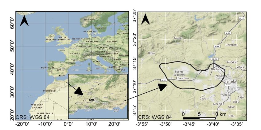
Palenzuela Baena, J.A.

 series follows the mainshock or the first earthquake with the highest magnitude, however, in an earthquake
 swarm, aftershocks can intensify after slowing down during a few hours or months. Swarms are associated
 with volcanic, geothermal or, as in this case, tectonic activity. In the target area, a similar sequence was
 recorded in 1979 [3] with maximum intensities of 6 in the modified Mercalli scale and a magnitude of 5 in
 the Richter scale [4]. Instead, during the more recent event of 2020-2021, only one earthquake reached a
 magnitude of 4.4 in the moment magnitude scale (Mw) [5] on 23 January 2021 in the northwest of Santa Fe
 with intensities reaching the levels V-VI. This earthquake exceeded the magnitude of 3.6 recorded in the
 previous earthquake on 2 December 2020 in the Lg wave phase-amplitude scale (mbLg) [6], with intensities
 IV-V [7].

 The geographical area of interest (AOI), targeted in this document, is located in the southern Spain to the
 northeast part of the Granada Basin (Figure 1).

 Figure 1. Geographical location of the AOI

 Southern Spain is the zone of this country with the highest seismicity, which is very noticeable in the
 Granada Basin, as registered by the historical earthquake record (Table 1). This active seismicity is
 conditioned by the convergence of the Eurasian and African plates, which has led the geologically rapid
 uplift of the Betic Cordilleras. This high uplift rate is well represented in the NE-SW antiform of Sierra
 Nevada, whose height exceeded more than 4000 m since 8-9 million years ago (late Miocene). As a result, a
 compressive stress field has been developed in the NNW-SSE direction with a tension field in the
 approximately orthogonal direction (ENE-WSW) [8,9].

 2

Palenzuela Baena, J.A.

 YEAR MAGNITUDE MAX. ZONE
 INTENSITY
 Jul. 1431 6.5 IX-X Atarfe-Granada
 4 Jul. 1526 -- VII-VIII Granada
 3 Sep. 1531 6.5 IX-X Baza (GR)
 27 Oct. 1806 5.9 VIII-IX Santa Fé (GR)
 25 Dec. 1884 6.8 X Arenas del Rey
 (GR)
 29 Dec. 1884 -- VII-VIII Arenas del Rey
 (GR)
 27 Jan. 1885 -- VII-VIII Alhama (GR)
 14 Mar. 1886 -- VII-VIII Loja (GR)
 31 May 1911 4.9 VII-VIII Santa Fé (GR)

 8 Jan. 1954 4.0 VII-VIII Arenas del Rey
 (GR)
 19 Apr. 1956 5.0 VIII Albolote (GR)
 Table 1. Historical record of the earthquakes with the highest magnitude in the province of Granada. Modified from
 [10].

 In addition to the structural and geophysical studies revealing the structural patterns of development, high-
 velocity rates are also well observed in southern Spain by the analysis of GNSS (global navigation satellite
 system) network data, reaching up to 4.5 mm/year to the south of Spain and North of Africa (area 1 in
 Figure 2) [11]. Consequently, NW-SE normal faults are favored by the tensional deformations. However, the
 complex tectonic mechanism of this area has made the extensional field more relevant. Especially, the
 geographical extension of the Sierra Nevada is dominated by a radial extension pattern as the majority of
 faults have performed as normal faults.

 3

Palenzuela Baena, J.A.

 Figure 2. Horizontal displacement velocity based on a GNSS network for the 2015-2018 interval. Taken from [11].

 Many of these fractures in the Granada Basin remain under the sediment as “blind” faults not identified on
 the ground surface. However, the length and depth of some of these faults have been determined through
 the analysis of seismological data [12]. A subset of the actual number of active faults affecting the Granada
 Basin is shown in Figure 3, extracted from the QAFI [13]. It should be noted that not all the faults of the QAFI
 are related to recent earthquakes, and many other faults that do not outcrop at the surface or are not yet
 identified can produce earthquakes.

 4

Palenzuela Baena, J.A.

 Figure 3. Active faults affecting the Granada Basin.

 As a result of this orogenic event, Granada and Guadix-Baza Basins were individualized from the sea during
 the late Neogene [14]. These basins have been sedimented, reaching a maximum depth of some 2600 m in
 the depocenter locate to the west of Sierra Elvira [15]. Accordingly, the combination of the sediment
 thickness (at the local scale) with tectonic episodes of differential displacements are the major factors
 triggering earthquakes in this tectonically active area. These seismic events release energy that is
 accommodated by the pre-existent faults at the borders and internally to the basins.

 In regard to the swarm event of 2020-2021, this paper represents a brief analysis of the findings derived
 from preliminary research based on an application of the InSAR (Synthetic Aperture Radar Interferometry)
 technique by using open resources. These resources are referred to as the Sentinel-1 imagery and the
 processing software SNAP [16]. InSAR consists of the change measurement in the signal phase between two
 images containing the same geographical area but acquired at different times. The signal phase changes as
 the ground moves and this effect are used to detect small ground displacements. However, the sensibility
 of this technique depends on the sensor specifications, acquisition geometry, and target characteristics. In
 the present application, InSAR is applied to three different consecutive periods covering swarm
 earthquakes of different magnitudes in the specified AOI, so the performance of this technique by using
 open resources can be evaluated.

 2. Materials and Methods
 2.1 Data

 For the purpose of the present analysis the following datasets have been obtained:

 5

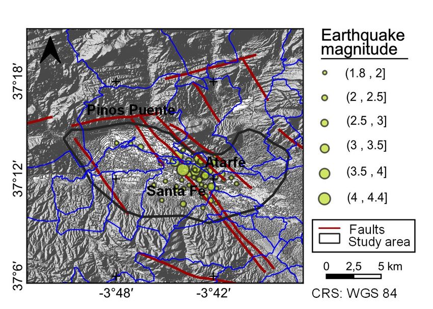
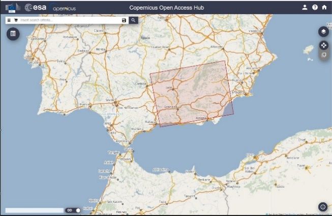
Palenzuela Baena, J.A.

 1 Five single look complex (SLC) images from the Sentinel-1 satellite (Table 2) to cover different periods
 running before and within the swarm event, to 25 Jan. 2021. More specifically, the Level-1 product of
 the Interferometric Wide Swath (IW) acquisition mode with dual vertical (DV) polarization (VV-VH) has
 been used here. These images, which are freely distributed, have been downloaded from the
 Copernicus Open Access Hub [17]. All of the selected images are in the ascending orbit with the line-of-
 sight (LOS) pointing to the Est (Figure 4).
 Image name Adquisition
 date
 S1A_IW_SLC__1SDV_20210125T181029_20210125T181056_036298_04422E_EB01 25/01/2021
 S1A_IW_SLC__1SDV_20210113T181030_20210113T181057_036123_043C1F_B5F4 13/01/2021
 S1A_IW_SLC__1SDV_20201208T181031_20201208T181058_035598_0429D8_CA67 08/12/2020
 S1A_IW_SLC__1SDV_20201126T181032_20201126T181059_035423_0423C7_4E74 26/11/2020
 S1A_IW_SLC__1SDV_20201114T181032_20201114T181059_035248_041DC4_5A2D 14/11/2020
 Table 2. Dataset of the satellite images used.

 Figure 4. Footprint of the satellite image dataset (left) and sketch of the LOS in descending and ascending orbits.

 2 A dataset including the earthquakes of magnitude higher than 1.8 from 14 Nov. 2020 to 25 Jan. 2021.
 This dataset has been downloaded from the Earthquake Catalogue [7]. Spatial distribution of the
 seismic dataset is shown in Figure 5a. Additionally, some delineations hypothetically belonging to the
 same fault planes have been highlighted in Figure 5b. The main criteria to digitize these traces is based
 on epicentres occurring closer in time and/or space in a quasi-straight linear path parallel to the NW-SE
 direction, which is consistent with the main orientation of the identified faults of the QAFI. As can be
 seen, the majority of the epicentres belonging to the earthquakes with the greater magnitude are
 located between the municipalities of Pinos Puente, Atarfe and Santa Fe, to the north part of the
 Granada Basin. This is a seismic active border that separates the basin sediments from a calcareous
 bedrock which is intensely fractured and faulted, that constitutes the mountainous relief of Sierra Elvira
 to the north of the Granada Basin.

 6

Palenzuela Baena, J.A.

 a

 b

 Figure 5. A) Spatial distribution and magnitude of the earthquake dataset. B) Enlarged view with delineations within
 hypothetical fault planes showing the period within which earthquakes occurred.

 7

Palenzuela Baena, J.A.

 The above-described dataset of satellite images has been processed with the following software:

 3 SNAP v6.0 [16], an open software created by the European Space Agency (ESA) for satellite imagery
 processing and analysis.

 4 QGIS v3.16.3 [18], an open-source Geographical Information System (GIS).

 5 The plugin SNAPHU v2.0.4 [19] for SNAP, an open-source software that transforms the interferometric
 phase into displacements.

 2.2 Methods

 Mapping the small deformation of large areas due to different phenomena (earthquakes, subsidence,
 volcanism, infrastructure failures, among others) it is possible by applying the well-known InSAR technique.
 InSAR consists of the processing of reflected radar signals which are collected in the off-nadir angle (or look
 angle) for the same area over different times. It enables the study of the deformation variation, which is
 useful for many applications such as infrastructure maintenance and natural risk management.

 A radar signal is characterized by amplitude and phase. The signal amplitude is related to the backscattered
 energy, which is highest for stiff and hard natural and artificial objects. In addition, phase depends on the
 sensor-to-target distance, and thus, it is used to estimate ground displacements along the LOS direction of
 the signal path.

 InSAR, or SAR lnterferometry, is the basic technique to measure the signal phase change between two
 different times over the same area as the distances between the sensor and ground points change, having a
 specific effect on the phase recorded by the sensor. It is focused on the interferogram generation from the
 phase difference between two SAR images, or the interferometric phase. To calculate this difference, Eq. (1)
 [20] is applied by taking into account a ground reference point.

 ∆∅ = + + + ∆∅ + ∆∅ Equation 1
 
 where:

 - λ: SAR wavelength

 - h: relative ground elevation of targets with respect to a horizontal reference plane

 - s: relative slant range position of targets

 - d: projection of the relative displacement of targets along the LOS

 - Bn: perpendicular baseline

 - R: SAR-target distance

 - Θ: “off-nadir” LOS angle

 - ΔΦAPS: atmospheric phase screen or differential tropospheric delay phase contribution

 8

Palenzuela Baena, J.A.

 - ΔΦλ: phase noise as results of the temporal and geometric decorrelation

 By using a digital elevation model (DEM) and precise orbital information, the first and second term of the
 interferometric phase can be calculated and subtracted. These terms are referred to the topographic phase
 and the so-called flat-earth phase related to the earth curvature, respectively. Thus, the term related to the
 target movement (d) can be extracted together with the atmospheric phase screen and the decorrelation
 noise (Eq. 2), obtaining the differential SAR interferometric phase (DINSAR).
 
 ∆∅ = d+ ∆∅ + ∆∅ Equation 2
 
 When solving the InSAR equations, two major problems appear. The first one is related to the phase
 ambiguity. Surface displacements are not directly derived from InSAR. However, the phase difference is
 determined as the position within one cycle (0° to 360°, 0 to 2π radians, or – π to π expressed as a
 sinusoidal function) corresponding to the 2-way travel of the radar signal when it goes to and returns from
 the target. That means that each repeating proportion of a wave cycle will produce the same measure,
 regardless of the number n of cycles (n2π) that cannot be directly measured, appearing the so-called phase
 ambiguity. It follows that from Eq. 2, the sensitivity to measures the maximum displacement will depend on
 the wavelength. Thus, a target displacement in the LOS direction of half-wavelength (λ/2) will result in the
 maximum movement being detected without considering decorrelation phase noise and APS effects
 (∆∅ = 2π).

 To determine the additional number of entire cycles to be added to the measured phase, the phase
 difference between neighbouring pixels has to be integrated through the “phase unwrapping” process [21].
 As an interferogram constitutes the two-dimensional map of phase differences respect a reference point,
 more than one cycle of complete cycles can appear as pixels locates far away from this point. This gives a
 series of colour fringes repeated for every phase cycle. The zones where the distance between the fringes
 of the same colour is closer correspond with greater surface deformation. A good example is shown in
 Figure 6, which shows the fringes generated by combining two Sentinel-1 radar images over the zone
 affected by the Earthquake (24 August 2016) of Central Italy with a magnitude of 6.1, near Amatrice.

 Figure 6. Interferogram showing clear fringes related to the Central Earthquake of Italy, occurred on 24 August 2016.
 Taken from [22].

 In this work the phase ambiguity problem is resolved by applying the Statistical-cost, Network-flow
 Algorithm for Phase Unwrapping implemented in the SNAPHU plugin [23], enabling the transformation from
 differential interferometric phase measurements to ground displacements.

 The second problem is related to the phase decorrelation noise, which is the more difficult part to be
 cancelled. In some cases, well and stable meteorological conditions facilitates to model and cancel the APS,
 as the atmospheric phase show a strong spatial correlation while the target motion is characterized by

 9

Palenzuela Baena, J.A.

 strong correlation in time. In addition, temporal decorrelation produces a phase noise when the return
 signal characteristics become extremely different with time as consequence of rapid changes occurring in
 the surface targets (vegetation, water, rapid landslides, among other). Temporal decorrelation can also
 result as a consequence of the geometric decorrelation related to the acquisition geometry (incidence
 angle) changes so the target reflectivity also varies between sequential acquisitions. This is reduced by
 selecting images with very similar acquisition geometries (e.g.: the same relative orbit). Additionally, to
 avoid the processing of areas with a poor signal-to-noise ratio (SNR), a threshold on the coherence is used.
 Coherence represents a quality measurement of the interferometric phase, which depends on the
 decorrelation or change in the scattering properties of the measured targets such as reflectance varying
 over time.

 In the present analysis, the following workflow has been performed to obtain the interferometric phase and
 the ground displacement by using the Sentinel-1 processing tools included in SNAP software:

 1 Extract the part of the image data (Sub -Swath and bursts) that cover the AOI with the VV
 polarization. VV polarization is selected here as it is proven to give acceptable results for ground
 displacement, with high amplitude and good SNR [24].

 2 Orbit correction by applying Precise Orbit Ephemerides (POEORB) to each image.

 3 Coregistration to resample the slave image to the reference acquisition geometry of the master
 image in slant- or ground-range coordinates, and the application of the Enhanced Spectral Diversity
 (ESD) operator to correct the azimuth shift in the slave image.

 4 Interferogram formation with sinusoidal values from -π to π, as well as the generation of the
 coherence map with values from 0 (null coherence) to 1 (maximum coherence).

 5 Subtract the flat-earth and topographic phases.

 6 Apply the Deburst operator that merges adjacent burst removing seamlines.

 7 Apply the Goldstein Phase Filtering to increase the quality of the fringes existing in the
 interferogram.

 8 Create a subset of the interferogram to constrain the analysis area to the AOI extension.

 9 Phase unwrapping by using the plugin SNAPHU.

 10 Phase to displacement conversion.

 11 Geocode the displacement raster into a map coordinate system by correcting SAR geometric
 distortions with the aid of a pre-existing DEM.

 12 Export the phase, coherence, and displacements measurements into netCDF files which are readable
 by the GIS software.

 As above mentioned, in this paper Sentinel-1 data have been used. Sentinel-1 satellites have an acquisition
 cycle of 12 days, although the same area is revisited every 6 days if the two satellites (1A and 1B) navigating
 in different orbits are considered [25]. The sensor of the Sentinel-1 satellites operates in the C-band, with a
 wavelength of approximately 5.6 cm and the incidence angle varies between 20° and 46° [26]. This is the

 10

Palenzuela Baena, J.A.

 parameter that constrains the maximum displacement of 2.8 (half of the wave roundtrip), coinciding with
 one complete sine wave cycle or one wavelength. Another characteristic limiting the smallest angular or
 linear separation between two objects that can be resolved by this sensor is its ground resolution. The
 mission Sentinel provides Level-1 products as SLC images with a moderate ground resolution of about 22 m
 in azimuth (parallel to the flight direction) and 3.5 m in range (perpendicular to the flight direction)
 directions [27].

 After the SAR products are generated, phase and displacements are projected into GIS layouts to compare
 results, considering three interferograms: before the seismic series, co-seismic with the earthquake on 2
 Dec. 2020 and, co-seismic with the earthquake on 23 Jan. 2021. It is worth noting that due to the use of
 single interferograms, InSAR is more susceptible to decorrelation than other techniques based on the
 statistical stability of the phase properties through a greater image dataset, commonly, a minimum of 20-25
 images [28,29]. Accordingly, to avoid results with a poor SNR, the pixels with a coherence less than 0.55
 were masked.

 3. Results

 In the following, the findings of this preliminary research are presented. As above mentioned, the results
 from this InSAR application consist of the interferometric phase and displacement mapping, considering the
 conditions of low to moderate magnitude co-seismic events, as well as a medium resolution and long-
 wavelength SAR signal. The interferometric (wrapped) phase is used here to identify the zones that were
 affected by the seismic deformation, while displacement maps show the spatial variation of the earthquake
 effect. Negative displacements are related to surface targets moving far away from the satellite in the LOS
 direction, generally related to downwards displacements (subsidence, settlement and mass movements,
 among others). On the contrary, positive displacements are related to those targets moving towards the
 satellite position (e.g.: swelling or mass movements). White pixels within the displacement maps have been
 used to represent the areas with a coherence below the threshold of 0.55.

 Accordingly, the interferograms and displacements are shown in Figures 7-10 for the following periods
 limited by the available SAR images:
 - 14 Nov. 2020 to 26 Nov. 2020 (Figure 7), which represents the pre-seismic analysis.

 - 26 Nov. 2020 to 08 Dec. 2020 (Figure 8), co-seismic with the starting of the earthquake swarm,
 containing the earthquake of magnitude 3.6 occurred on 2 December 2020.

 - 13 Jan. 2021 to 25 Jan. 2021 (Figure 9-10), co-seismic with the earthquake of magnitude 4.4
 occurred on 23 January 2021.

 The results of the first period (Figure 7) do not show any phase patterns reflecting co-seismic phenomena.
 They only reveal some parts where the interferometric phase class matches the highest relief, such as the
 blue isolated zone to the north of the AOI, which coincides with the mountain of Sierra Elvira (municipality
 of Atarfe). Nonetheless, in general, displacements are closer to 0 m, matching a period of seismic
 quiescence before the starting of the earthquake series.

 11

Palenzuela Baena, J.A.

 Figure 7. Interferogram (top) and displacement map for the period 14 Nov. 2020 – 26 Nov. 2020 (bottom).

 The first signs of change appear in the following period when earthquakes of magnitudes up to 3.6 were
 recorded (Figure 8). It has to be noted, however, that the distribution of displacements is skewed to the
 positive domain, with lesser magnitudes to the northwest part of the AOI between the municipalities of
 Pinos Puente and Atarfe.

 12

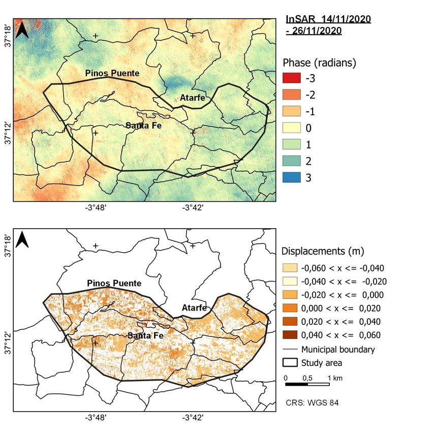
Palenzuela Baena, J.A.

 Figure 8. Interferogram (top) and displacement map for the period 26 Nov. 2020 – 08 Dec. 2020 (bottom).

 Ground changes are even more remarkable considering the last period is considered (Figure 8), including
 the earthquake of the highest magnitude (4.4). Its corresponding interferogram shows well-formed fringes
 with wide colour bands, indicating low displacement values. The yellow class is better evidenced to the
 north (Santa Fe - Atarfe) and northwest (Pinos Puente) of the AOI. This class represents downward
 movements reaching more than 2 cm, measurements which have not documented or measured with other
 techniques to date and could be overestimated here for the low to moderate magnitudes of the earthquake
 swarm.

 13

Palenzuela Baena, J.A.

 Figure 9. Interferogram (top) and displacement map for the period 13 Jan. 2021 – 25 Dec. 2021 (bottom).

 Despite the limitations of this preliminary application, and given the highest effect related to the 23 January
 earthquake with magnitude 4.4, together with others of lower magnitude, the displacements generated
 during the last analysed period (13 Jan. 2021 – 25 Dec. 2021) were then standardized. This was carried out
 by applying a simple custom script, coded with the QGIS Python console to produce values between -1
 (highest negative displacement) and 1 (highest positive displacement). In this way, values are rescaled to be
 represented into 8 classes, thus enhancing the relative displacement within the AOI. The standardized
 displacement map is shown in Figure 10. It can be observed the highest values within the interval (-1, 0.75]
 located in the municipalities of Pinos Puente, Atarfe and Santa Fe. In addition, the standardized map is
 characterized by a generalization of the negative values, which represent a downward movement, similar to
 a settlement.

 14

Palenzuela Baena, J.A.

 Figure 10. Interferogram (top) and standardized displacement map for the period 13 Jan. 2021 – 25 Dec. 2021.

 Discussion and conclusions

 The present document constitutes a brief application of InSAR through the use of open resources with the
 aim of mapping the ground movement effects in relation to the 2020-2021 earthquake swarm in the district
 of La Vega, which is located in the province of Granada to the south of the Iberian Peninsula. For this scope,
 the available open data from the Sentinel-1 satellite constellation were exploited, even though low to
 moderate magnitude earthquakes together with the medium resolution and long-wavelength SAR signal are
 expected to decrease the sensitivity of this technique. Under these considerations, three periods were
 evaluated by generating one pre-seismic and two co-seismic interferograms leveraging the processing
 utilities of SNAP and the plugin SNAPHU.

 15

Palenzuela Baena, J.A.

 Interferometric results were then imported and analysed into QGIS. In general, the pre-seismic period did
 not show ground movement evidence, while an incremental development of fringes appears with the
 increasing magnitude of the earthquakes in the second and third periods. The highest displacements were
 detected in the third period, containing the earthquake of 4.4 with an epicenter in the municipality of Santa
 Fe. These displacements are distributed between the municipalities of Pinos Puente, Atarfe and Santa Fe,
 matching some of the areas documented as being damaged with the highest intensities, and reaching the
 levels IV-V [30,31] and even VI [7]. Taking into account the InSAR results after processing the Sentinel-1
 dataset, the highest downward displacements show values that exceed 2 cm.

 However, it has to be noted that, even though the pixels showing low coherence were filtered, residual
 phase is still detected as a consequence of the noise produced by atmospheric and decorrelating factors in
 the area. This can derivate in erroneous or skewed displacements, as those observed in the second period.
 The total cancellation of the noisy phase is a difficult task, and although deeper processing can be tried, it
 will not guarantee the improvement of the interferometric phase.

 Definitely, the use of open resources for InSAR data processing provides a relevant tool for ground
 monitoring and the generation of preliminary maps of the seismic effects at a territorial scale that cannot
 be reached by other techniques (DGPS, continue total station measurement, among others) at a low cost.
 This is a useful instrument to evaluate seismic risk, which strongly depends on the vulnerability of the
 constructions, as well as on the susceptibility of the geological settings (sediment and rock strength against
 external actions, and hydrogeological characteristics). Further research can be done to correlate or model
 the ground deformation with the dynamical (earthquake acceleration, hydrogeological variables) and static
 factors (lithology), so the expected damages by earthquakes of greater magnitudes can be estimated.
 Additionally, more precise maps and point measurements can be obtained if high-resolution images and
 complex techniques based on DInSAR are applied. One of the most often used techniques is the Persistent
 Scatterer Interferometry (PSI), based on the analysis of a longer time-series of SAR images, so pixels
 maintaining a statistically highest coherence throughout the entire series (persistent scatterer) are selected
 for the processing of the interferometric phase and displacements. This technique, combined with the
 highest resolution images as those from the Cosmo-SkyMed (Cosmo SkyMed COnstellation of small
 Satellites for the Mediterranean basin Observation), can provide precise and useful information for building
 and infrastructure monitoring and natural risk management [32]. Thus, a database on time-series of
 subcentimetric displacements can be generated to make it available to practitioners, scientists and
 researchers, as can be revised in recent European initiatives [33].

 References
1. ABCAndalucía. El enjambre sísmico que causa los terremotos en Granada puede durar «semanas o meses», según los
 expertos. Availabe online: https://sevilla.abc.es/andalucia/granada/sevi-enjambre-sismico-lugar-terremotos-granada-
 puede-durar-semanas-segun-expertos-202101271019_noticia.html?ref=https:%2F%2Fwww.google.com%2F
 (accessed on 05/04/2021).
2. El Confidencial. Los terremotos continuarán en Granada... En 1979, fueron seis meses de sismos en cadena. Availabe
 online: https://www.elconfidencial.com/espana/andalucia/2021-01-28/terremotos-continuaran-granada-1979-seis-
 meses-sismos_2925700/ (accessed on 05/04/2021).
3. IDEAL. 1979: el 'espejo' de los terremotos de Granada en 2021. Availabe online:
 https://www.ideal.es/granada/granada-dejo-temblar-1979-terremotos-20210128113505-nt.html (accessed on
 05/04/2021).
4. Richter, C.F. An instrumental earthquake magnitude scale. Bulletin of the seismological society of America 1935, 25,
 1-32.
5. Hanks, T.C.; Kanamori, H. A moment magnitude scale Journal of Geophysical Research 1979, 84, 23480-23500.

 16

Palenzuela Baena, J.A.

6. López, C. Nuevas fórmulas de magnitud para la Península Ibérica y su entorno. Trabajo de investigación del Máster
 en Geofísica y Meteorología; Departamento de Física de la Tierra, Astronomía y Astrofísica I. Universidad
 Complutense de Madrid. Madrid, 2008.
7. Instituto Geográfico Nacional. Catálogo de terremotos. Availabe online: https://www.ign.es/web/ign/portal/sis-
 catalogo-terremotos (accessed on 30/01/2021).
8. Sanz de Galdeano, C.; López-Garrido, A.C. Nature and impact of the Neotectonic deformation in the western Sierra
 Nevada (Spain). Geomorphology 1999, 30, 259-272, doi:https://doi.org/10.1016/S0169-555X(99)00034-3.
9. Sanz de Galdeano, C.; Shanov, S.; Galindo-Zaldívar, J.; Radulov, A.; Nikolov, G. A new tectonic discontinuity in the
 Betic Cordillera deduced from active tectonics and seismicity in the Tabernas Basin. Journal of Geodynamics 2010,
 50, 57-66, doi:https://doi.org/10.1016/j.jog.2010.02.005.
10. IAGPDS. Instituto Andaluz de Geofísica y Prevención de Desastres Sísmicos. Terremotos históricos del sur de
 España. Availabe online: http://iagpds.ugr.es/pages/informacion_divulgacion/terremotos_historicos (accessed on
 26/02/2021).
11. Pena, S. Present-day 3D GPS velocity field of the Iberian Peninsula and implications for seismic hazard. In Master
 Oficial en Recursos Minerals i Riscos Geologics. Specialty: Geological Hazards, Universitat Autonoma de Barcelona,
 Facultat de Geologia, 2018.
12. Serrano, I.; Zhao, D.; Morales, J. 3-D crustal structure of the extensional Granada Basin in the convergent boundary
 between the Eurasian and African plates. Tectonophysics 2002, 344, 61-79, doi:https://doi.org/10.1016/S0040-
 1951(01)00201-3.
13. García Mayordomo, J.; Insua-Arévalo, J.; Martinez-Diaz, J.; Jiménez-Díaz, A.; Martín Banda, R.; Martín-Alfageme,
 S.; Álvarez-Gómez, J.; Rodríguez-Peces, M.; Perez-Lopez, R.; Rodriguez-Pascua, M., et al. The Quaternary active
 faults database of Iberia (QAFI v.2.0). Journal of Iberian Geology 2012, 38, 285-302,
 doi:10.5209/rev_JIGE.2012.v38.n1.39219.
14. Saez de Galdeano, C.; García-Tortosa, F.J.; Peláez, J.A.; Alfaro, P.; Azañón, J.M.; Galindo-Zaldívar, J.; Casado, C.L.;
 Garrido, A.C.L.; Rodríguez-Fernández, J.; Ruano, P. Main active faults in the Granada and Guadix-Baza Basins (Betic
 Cordillera)/Principales fallas activas de las Cuencas de Granada y Guadix-Baza (Cordillera Bética). Journal of Iberian
 Geology 2012, 38, 209-223.
15. Morales, J.; Vidal, F.; De Miguel, F.; Alguacil, G.; Posadas, A.M.; Ibañez, J.M.; Guzmán, A.; Guirao, J.M. Basement
 structure of the Granada basin, Betic Cordilleras, southern Spain. Tectonophysics 1990, 177, 337-348,
 doi:https://doi.org/10.1016/0040-1951(90)90394-N.
16. ESA. S1TBX - ESA Sentinel-1 Toolbox. Availabe online: http://step.esa.int (accessed on 05/04/2021).
17. Copernicus Open Access Hub. Availabe online: https://scihub.copernicus.eu/dhus/#/home (accessed on 15/02/2021).
18. QGIS.org, QGIS Geographic Information System. QGIS Association. Availabe online: http://www.qgis.org (accessed
 on 5/02/2021).
19. SNAPHU: Statistical-Cost, Network-Flow Algorithm for Phase Unwrapping. Availabe online:
 https://web.stanford.edu/group/radar/softwareandlinks/sw/snaphu/ (accessed on 05/02/2021).
20. Prati, C.; Ferretti, A.; Perissin, D. Recent advances on surface ground deformation measurement by means of repeated
 space-borne SAR observations. Journal of Geodynamics 2010, 49, 161-170,
 doi:https://doi.org/10.1016/j.jog.2009.10.011.
21. Goldstein, R.; Zebker, H.; Werner, C. Satellite Radar Interferometry: Two-Dimensional Phase Unwrapping. Radio
 Science 1988, 23, doi:10.1029/RS023i004p00713.
22. Earth Galery. Sentinel-1 radar data interferogram (15.08.2016 and 27.08.2016), Italy, © 2016 Copernicus Sentinel
 data/ESA/CNR-IREA. Availabe online:
 http://www.gisat.cz/content/a_render/20?act_snimek=127&template=layout_home_archive (accessed on
 06/04/2021).
23. Chen, C.W.; Zebker, H.A. Network approaches to two-dimensional phase unwrapping: intractability and two new
 algorithms. J. Opt. Soc. Am. A 2000, 17, 401-414, doi:10.1364/JOSAA.17.000401.
24. Vaka, D.S.; Sharma, S.; Rao, Y. Comparison of HH and VV Polarizations for Deformation Estimation using Persistent
 Scatterer Interferometry; 2017.
25. Sentinel Online. Geograhical Coverage. Availabe online: https://sentinel.esa.int/web/sentinel/missions/sentinel-
 1/satellite-description/geographical-coverage (accessed on 05/04/2021).
26. Sentinel-1. SAR Instrument. Availabe online: https://sentinels.copernicus.eu/web/sentinel/technical-guides/sentinel-
 1-sar/sar-instrument (accessed on 05/04/2021).
27. Sentinel Online. Level-1 Interferometric Wide Swath SLC Products. Availabe online:
 https://sentinel.esa.int/web/sentinel/technical-guides/sentinel-1-sar/products-algorithms/level-1/single-look-
 complex/interferometric-wide-swath (accessed on 05/04/2021).

 17

Palenzuela Baena, J.A.

28. Crosetto, M.; Monserrat, O.; Cuevas-González, M.; Devanthéry, N.; Crippa, B. Persistent Scatterer Interferometry: A
 review. ISPRS Journal of Photogrammetry and Remote Sensing 2016, 115, 78-89,
 doi:https://doi.org/10.1016/j.isprsjprs.2015.10.011.
29. Jia, H.; Liu, L. A technical review on persistent scatterer interferometry. Journal of Modern Transportation 2016, 24,
 153-158, doi:10.1007/s40534-016-0108-4.
30. El Independiente de Granada. El terremoto más sentido en Granada en 40 años deja un herido y numerosos daños en
 viviendas. Availabe online: http://www.elindependientedegranada.es/ciudadania/terremoto-mas-sentido-granada-40-
 anos-deja-herido-numerosos-danos-viviendas (accessed on 05/04/2021).
31. SUR. Un terremoto de magnitud 4,4 con epicentro en Santa Fe deja daños materiales y un herido. Availabe online:
 https://www.diariosur.es/andalucia/terremoto-magnitud-epicentro-santa-deja-danos-materiales-herido-
 20210123164106-ga.html#imagenNaN (accessed on 05/04/2021).
32. D’Aranno, P.J.V.; Di Benedetto, A.; Fiani, M.; Marsella, M.; Moriero, I.; Palenzuela Baena, J.A. An Application of
 Persistent Scatterer Interferometry (PSI) Technique for Infrastructure Monitoring. 2021, 13, 1052,
 doi:https://doi.org/10.3390/rs13061052.
33. Satellite Services for Structural Monitoring - I.MODI. Availabe online: https://www.imodi.info/en/home-en/
 (accessed on 05/02/2021).

 18