Re-thinking EEG-based non-invasive brain interfaces: modeling and analysis
←
→
Page content transcription
If your browser does not render page correctly, please read the page content below
Re-thinking EEG-based non-invasive brain interfaces: modeling and analysis

                                                                                Gaurav Gupta˚ , Sérgio Pequito: and Paul Bogdan˚
                                                   ˚ Ming  Hsieh Department of Electrical Engineering, University of Southern California, Los Angeles, CA, USA
                                                                                       Email: {ggaurav, pbogdan}@usc.edu
                                                        : Department of Industrial and Systems Engineering, Rensselaer Polytechnic Institute, Troy, NY, USA
                                                                                              Email: goncas@rpi.edu
arXiv:1803.10318v1 [q-bio.NC] 27 Mar 2018

                                               Abstract—Brain interfaces are cyber-physical systems that         goal, Facebook has invested in developing new non-invasive
                                            aim to harvest information from the (physical) brain through         optical imaging technology that is five times faster and
                                            sensing mechanisms, extract information about the underlying         portable with respect to the one available on the market
                                            processes, and decide/actuate accordingly. Nonetheless, the
                                            brain interfaces are still in their infancy, but reaching to their   and would possess increased spatial and temporal resolution.
                                            maturity quickly as several initiatives are released to push         Nonetheless, these are just some of the initiatives among
                                            forward their development (e.g., NeuraLink by Elon Musk and          others by some big Silicon Valley players that want to
                                            ‘typing-by-brain’ by Facebook). This has motivated us to revisit     commercialize brain technologies [3].
                                            the design of EEG-based non-invasive brain interfaces. Specif-          Part of the motivation for the ‘hype’ in the use of
                                            ically, current methodologies entail a highly skilled neuro-
                                            functional approach and evidence-based a priori knowledge            neurotechnologies – both invasive and non-invasive brain in-
                                            about specific signal features and their interpretation from         terfaces – is due to their promising application domains [4]:
                                            a neuro-physiological point of view. Hereafter, we propose to        (i) replace, i.e., the interaction of the brain with a wheelchair
                                            demystify such approaches, as we propose to leverage new             or a prosthetic device to replace a permanent functionality
                                            time-varying complex network models that equip us with a             loss, (ii) restore, i.e., to bring to its normal use some
                                            fractal dynamical characterization of the underlying processes.
                                            Subsequently, the parameters of the proposed complex network         reversible loss of functionality such as walking after a severe
                                            models can be explained from a system’s perspective, and, con-       car accident or limb movement after a stroke, (iii) enhance,
                                            secutively, used for classification using machine learning algo-     i.e., to enable to outperform in a specific function or task, as
                                            rithms and/or actuation laws determined using control system’s       for instance an alert system to drive for long periods of time
                                            theory. Besides, the proposed system identification methods          while attention is up; and (iv) supplement as in equipping
                                            and techniques have computational complexities comparable
                                            with those currently used in EEG-based brain interfaces,             one with extra functionality, as a third arm to be used during
                                            which enable comparable online performances. Furthermore,            surgery. Notwithstanding, these are just some of the (known)
                                            we foresee that the proposed models and approaches are               potential uses of neurotechnology.
                                            also valid using other invasive and non-invasive technologies.          Despite the developments and promise of future applica-
                                            Finally, we illustrate and experimentally evaluate this approach     tions of brain interfaces (some of which we cannot currently
                                            on real EEG-datasets to assess and validate the proposed
                                            methodology. The classification accuracies are high even on          conceive), we believe that current approaches to both inva-
                                            having less number of training samples.                              sive and non-invasive brain interfaces can greatly benefit
                                                                                                                 from cyber-physical systems (CPS) oriented approaches and
                                              Keywords-brain interfaces; spatiotemporal; fractional dy-
                                            namics; unknown inputs; classification; motor prediction             tools to increase their efficacy and resilience. Hereafter, we
                                                                                                                 propose to focus on non-invasive technology relying on
                                                                                                                 electroencephalogram (EEG) and revisit it through a CPS
                                                                  I. I NTRODUCTION
                                                                                                                 lens. Moreover, we believe that the proposed methodology
                                               We have recently testimony a renewed interest in invasive         can be easily applicable to other technologies, e.g., electro-
                                            and non-invasive brain interfaces. Elon Musk has released            magnetic fields (magnetoencephalography (MEG) [5], and
                                            the NeuraLink initiative [1] that aims to develop devices            the hemodynamic responses associated to neural activity,
                                            and mechanisms to interact with the brain in a symbiotic             e.g. functional magnetic resonance imaging (fMRI) [6],
                                            fashion, thus merging the artificial intelligence with the           [7], and functional near-infrared spectroscopy (fNIRS) [8]).
                                            human brain. The potential is enormous since it would                Nonetheless, these technologies present several drawbacks
                                            ideally present a leap in our understanding of the brain, and        compared to EEG, e.g., cost, scalability, and user comfort,
                                            an unseen enhancement of its functionality. Alternatively,           which lead us to focus on EEG-based technologies. Similar
                                            Facebook just announced the ‘Typing-by-Brain’ project [2]            argument can be applied in the context of non-invasive
                                            that gathered a team of 60 researchers whose target is to            versus invasive technologies that require patient surgery.
                                            be capable of writing 100 words per minute that contrasts               Traditional approach to EEG neuroadaptive technology
                                            with the state-of-the-art of 0.3 to 0.82 words per minute            consists of proceeding through the following steps [9],
                                            assuming an average of 5 letters per word. Towards this              [10]: (a) signal acquisition (in our case, measurement of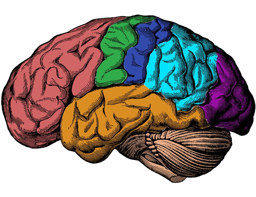
feature                     machine learning
                                                                  extraction                    classification
                             EEG time series                                                                          predicted
                                                                                                                      motor task

   EEG channels

                                                                   real time processing of time series
                                                                   for machine learning classification

Figure 1: A systematic process flow of the Brain interface. The imagined motor movements of the subject are captured in the
form of EEG time series which are then fed to the computational unit. A fractional-order dynamics based complex network
model is estimated for the time series and the model parameters are used as features for machine learning classification.
The output of classifier predicts various motor movements with certain confidence.

the EEG time-series); (b) signal processing (e.g., filtering       known stimuli, e.g., artifacts or inter-region communication.
with respect to known error sources); (c) feature extraction       A. Related Work and Novel Contributions
(i.e., an artificial construction of the signal that aims to
                                                                      We put forward that the ability to properly model the EEG
capture quantities of interest); (d) feature translation (i.e.,
                                                                   time-series with complex network models, that account for
classification of the signal according to some plausible
                                                                   realistic setups, can enable the brain interfaces methods to
neurophysiological hypothesis); and (e) decision making
                                                                   get transformed from detectors to decoders. In other words,
(e.g., provide instructions to the computer to move a cursor,
                                                                   we do not want to solely look for the existence of a peak
or a wheelchair to move forward) – see also Figure 1 for an
                                                                   of activity in a given band that is believed to be associated
overview diagram.
                                                                   with a specific action. But we want to decompose the bunch
   In this paper, we propose to merge steps (b) and (c)            of signals into different features, i.e., parameters of our
motivated by the fact that these often accounts for spatial        complex network model, that are interpretable. Thus, al-
or temporal properties, and are only artificially combined         lowing us to understand how different regions communicate
in a later phase of the pipeline, i.e., at step (d) of fea-        during a specific action/task by representing them as nodes
ture translation. First, we construct a time-varying complex       of the complex network and estimating the dependence via
network where the activity of nodes (or EEG signal) have           coupling matrix. The node activities are assumed to be
long-range memory and the edges accounts for inter-node            evolving at different time-scales and in the general setup of
spatial dependence. Thus, we argue that the previous ap-           presence of external stimuli which could either be unwanted
proach discards several spatial-temporal properties that can       noise or external process driving the system. In engineering,
be weighted for signal processing and feature extraction           this will enable us to depart from a skill dependent situation
phases. In other words, current EEG brain interfaces require       to general context analysis, which will enhance the resilience
one to have an understanding of the different regions of           of the approaches for practical nonsurgical brain interfaces.
the brain responsible. For instance, regions for motor or          Besides, it will equip bioengineers, neuroscientists, and
visual actions, as well as artificial frequency bands that are     physicians with an exploratory tool to pursue new technolo-
believed to be more significant for a specific action (also        gies for neuro-related diagnostics and treatments, as well as
known as evidence-based). Besides, one needs to understand         neuro-enhancement.
and anticipate the most likely causes noise/artifacts in the          The proposed approach departs from those available in the
EEG data collected and filter out entire frequency bands,          literature, see [4], [9], [10] and references therein. In fact, to
which possibly compromises phenomena of interest not               the best of authors’ knowledge, in the context of noninvasive
being available for post-processing. Instead, we propose a         EEG-based technologies, [11] is the only existing work that
modeling capability to enable the modeling of long-range           explores fractional-order models in the context of single-
memory time-series that at the same time accounts for un-          channel analysis, which contrasts with the spatiotemporal
modeled leveraged in this paper that copes with multi- model’s parameters, and in Section II-D we describe how to
channel analysis. Furthermore, the methodology presented interpret them for the classification task.
in this paper also accommodate unknown stimuli [12].
For which efficient algorithms are proposed and leveraged A. EEG-based Technology for Brain Interfaces: a brief
hereafter to simultaneously retrieve the best model that overview
conforms with unknown stimuli, and separating the unknown EEG enables the electrophysiological monitoring of
stimuli from the time-series associated with brain activity. space-averaged synaptic source activity from millions of
Our methods are as computationally efficient and stable as neurons occurring at the neocortex level. The EEG signals
least-squares and spectral analysis methods used in a spatial have a poor spatial resolution but high temporal resolution,
and temporal analysis, respectively; thus, suitable for online since the electrical activity generated at the ensemble of
implementation in nonsurgical brain interfaces. neurons level arrives at the recording sites within mil-
The main contributions of the present paper are those liseconds. The electrodes (i.e., sensor) are placed over an
of leveraging some of the recently proposed methods to area of the brain of interest, being the most common the
develop new modeling capabilities for the EEG based neuro- visual, motor, sensory, and pre-frontal cortices. Usually, they
wearables that are capable of enhancing the signal quality follow standard montages – the International 10-20 system
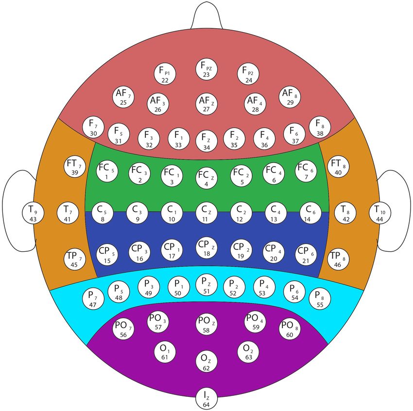
and decision-making. Furthermore, the parametric descrip- is depicted in Figure 2.
tion of these models provides us with new features that are Most of the activity captured by the EEG electrodes is
biologically motivated and easier to translate in the context due to the interactions between inhibitory interneurons and
of brain function associated with a signal characterization, excitatory pyramidal cells, which produces rhythmic fluctu-
and free of signal artifacts. Thus, making the brain-related ations commonly referred to as oscilations. The mechanisms
activity interpretable, which leads to resilient and functional that generate those oscillations is not yet completely under-
nonsurgical brain interfaces. stood, but it has been already identified that some ‘natural
oscillations’ provide evidence of activity being ‘processed’
B. Paper Organization in certain regions of the brain at certain ‘frequencies’.
The remaining of the paper is organized as follows. Sec- Therefore, oscillatory behavior of human brain is often
tion II introduces the complex network model considered in partitioned in bands (covering a wide range of frequencies
this paper and the main problem studied in this manuscript. decaying as 1{f in power): (i) δ-band (0.5-3Hz); (ii) θ-band
Also we will see the description of the employed method (3.5-7Hz); (iii) α-band (8-13Hz); (iv) β-band (14-30Hz); and
for feature selection and then classification techniques. In (v) γ-band (30-70Hz). Furthermore, there has been some
Section III, we present an elaborated study on the different evidence that activity in certain bands is associated with
datasets taken from the BCI competition [13]. sensory registration, perception, movement and cognitive
processes related to attention, learning and memory [14]–
II. R E - THINKING EEG- BASED NON - INVASIVE [16]. Notwithstanding, such associations are often made
BRAIN INTERFACES
using correlation and/or coherence techniques that only
Brain interfaces aim to address the following problem. capture relationships between specific channels. But such
Is it possible to classify a specific cognitive state, e.g., mo- methods are not able to assess the causality between signals
tor task or its imagination, by using measurements collected that enables forecasting on the signal evolution, captured by
with a specific sensing technology that harvest information a model-based representation as we propose to do hereafter.
about brain activity? Different changes in the signals across different bands
In the current manuscript, we revisit this problem in the are also used to interpret the event-related potentials (ERPs)
context of brain-computer interfaces (BCI), when dealing in the EEG signals, i.e., variations due to specific events –
with EEG-based noninvasive brain interfaces. Towards this see [4] for detailed analysis. In the context of sensory-motor
goal, we review the currently adopted procedures for solving data used in the current manuscript to validate the proposed
this problem (see Figure 1 for an overview), and propose methodology, sensorimotor rhythms (SMRs) are often con-
a systems’ perspective that enables to enhance the BCI sidered. These represent oscillations that are recorded over
reliability and resilience. Therefore, in Section II-A we pro- the posterior frontal and anterior parietal areas of the brain,
vide a brief overview of the EEG-based technology and the i.e., over the sensorimotor cortices (see Figure 2). SMRs
connection with the brain-areas’ function associated with occur mainly in the α-band (for sensors located on the top of
studies conducted in the past. Next, in Section II-B, we in- the motor cortices), and on beta and lower gamma for those
troduce the spatiotemporal fractional model under unknown on the sensorimotor cortices [17]. Consequently, these have
stimuli. This will be the core of the proposed approach in been used as a default feature for classification of motor-
this manuscript to retrieve new features for classification, related execution and only the imagination of performing a
and, subsequently, enhancing brain interfaces capabilities. motor task. Notwithstanding, the spatiotemporal modeling is
In Section II-C, we describe how to determine the system simultaneously captured through direct state-space modelingcortex
cortex
sensory
motor
parietal
frontal lobe
lobe
temporal occipital
lobe lobe
Figure 2: Description of the brain functional regions and their corresponding location with respect to the EEG sensor cap.
that enables the system’s understanding of the dynamics of used as the discrete version of the derivative, for example
the underlying process. In addition, it provides a new set ∆1 xrks “ xrks ´ xrk ´ 1s. As evident, the difference
of attributes that can be used to improve feature translation, order of 1 has only one-step memory, and hence the classic
i.e., classification. linear-time invariant models are not able to answer the
B. Spatiotemporal Fractional Model with Unknown Stimuli long-range memory property of several physiological signals
as discussed before. On the other hand, the expansion of
A multitude of complex systems exhibit long-range (non- fractional-order derivative in the discretized setting [33] for
local) properties, interactions and/or dependencies (e.g., any ith state p1 ď i ď nq can be written as
power-law decays in memories). Example of such systems
k
includes Hamiltonian systems, where memory is the result ÿ
of stickiness of trajectories in time to the islands of regular ∆αi xi rks “ ψpαi , jqxi rk ´ js, (2)
j“0
motion [18]. Alternatively, it has been rigorously confirmed
that viscoelastic properties are typical for a wide variety of where αi is the fractional order corresponding to the ith
Γpj´αi q
biological entities like stem cells, liver, pancreas, heart valve, state and ψpαi , jq “ Γp´α with Γp.q denoting the
i qΓpj`1q
brain, muscles [18]–[26], suggesting that memories of these gamma function. We can observe from (2) that fractional-
systems obey the power law distributions. These dynam- order derivate provide long-range memory by including all
ical systems can be characterized by the well-established xi rk ´ js terms. A quick comparison between the prediction
mathematical theory of fractional calculus [27], and the accuracy of fractional-order derivative model and linear-time
corresponding systems could be described by fractional invariant model is shown in Figure 3. The fractional-order
differential equations [28]–[32]. However, it is until recently model can cope with sudden changes in the signals while
that fractional order system (FOS) starts to find its strong the linear model cannot.
position in a wide spectrum of applications in different We can also describe the system by its matrices tuple
domains. This is due to the availability of computing and pα, A, B, Cq of appropriate dimensions. The coupling matrix
data acquisition methods to evaluate its efficacy in terms of A represents the spatial coupling between the states across
capturing the underlying system states evolution. time while the input coupling matrix B determines how
Subsequently, we consider a linear discrete time inputs are affecting the states. In what follows, we assume
fractional-order dynamical model under unknown stimuli that the input size is always strictly less than the size of state
(i.e., inputs) described as follows: vector, i.e., p ă n.
∆α xrk ` 1s “ Axrks ` Burks Having defined the system model, the system identifica-
tion, i.e., estimation of model parameters, from the given
yrks “ Cxrks, (1)
data is an important step. It becomes nontrivial when we
n p
where x P R is the state, u P R is the unknown input and have unknown inputs since one has to be able to differentiate
y P Rn is the output vector. The differencing operator ∆ is which part of the evolution of the system is due to its300
observed
estimate the fractional order α using the wavelet technique
200 fractional
linear
described in [34]; and (ii) with α known, the z in equation
Neural Activity
100 (3) is computed under the additional assumption that the
0 system matrix B is known. Therefore, the problem now
-100 reduces to estimate A and the inputs turksut`T t
´2
. Towards
-200 this goal, we exploit the algorithm similar to expectation-
-300
maximization (EM) [35] from [12]. Briefly, the EM algo-
100 150 200 250 300 350 400 450 500
Sample ID
rithm is used for maximum likelihood estimation (MLE)
of parameters subject to hidden variables. Intuitively, in
Figure 3: Comparison of observed experimental EEG data our case, in Algorithm 1, we estimate A in the presence
with the prediction from fractional-order model and linear- of hidden variables or unknown unknowns turksut`T ´2
.
t
time invariant model. Therefore, the ‘E-step’ is performed to average out the
effects of unknown unknowns and obtain an estimate of
u, where due to the diversity of solutions, we control the
intrinsic dynamics and what is due to the unknown inputs. sparsity of the inputs using the parameter λ1 . Subsequently,
Subsequently, the analysis part that we need to address is the ‘M-step’ can then accomplish MLE estimation to obtain
that of system identification from the data, as described next. an estimate of A.
C. Data driven system identification It was shown theoretically in [12] that the algorithm is
convergent in the likelihood sense. It should also be noted
The problem consists of estimating α, A and inputs
that the EM algorithm can converge to saddle points as
turksut`T
t
´2
from the given limited observations yrks, k “
exemplified in [35]. The Algorithm 1 being iterative is cru-
rt, t ` T ´ 1s, which due to the dedicated nature of sensing
cially dependent on the initial condition for the convergence.
mechanism is same as xrks and under the assumption that
We will see in Section III that the convergence is very fast
the input matrix B is known. The realization of B can
making it suitable for online estimation of parameters.
be application dependent and is computed separately using
experimental data – as we explore later in the case study,
see Section III. For the simplicity of notation, let us denote Algorithm 1: EM algorithm
zrks “ ∆α xrk ` 1s with k chosen appropriately. The Input: xrks, k P rt, t ` T ´ 1s and B
pre-factors in the summation in (2) grows as ψpαi , jq „ Output: A and turksut`T t
´2
Opj ´αi ´1 q and, therefore, for the purpose of computational Initialize compute α using [34] and then zrks. For
ease we would be limiting the summation in (2) to J values, l “ 0, initialize Aplq as
where J ą 0 is sufficiently large. Therefore, zi rks can be plq
ai “ arg min ||Zi ´ Xa||22
written as a
J´1
ÿ repeat
zi rks “ ψpαi , jqxrk ` 1 ´ js, (3) (i) ‘E-step’: For k P rt, t ` T ´ 2s obtain urks as
j“0
urks “ arg min ||zrks ´ Aplq xrks ´ Bu||22 ` λ1 ||u||1 ,
with the assumption that xrks, urks “ 0 for k ď t´1. Using u
the above introduced notations and the model definition in where λ “ 2σ 2 λ;
1
(1), the given observations can be written as (ii) ‘M-step’:
pl`1q pl`1q pl`1q
zrks “ Axrks ` Burks ` erks, (4) obtain Apl`1q “ ra1 , a2 , . . . , an sT where
pl`1q
where e „ N p0, Σq is assumed to be Gaussian noise inde- ai “ arg min ||Z̃i ´ Xa||22 ,
a
pendent across space and time. For simplicity we would as-
sume that Σ “ σ 2 I. Also, let us denote the system matrices and Z̃i “ Zi ´ U bi ;
as A “ ra1 , a2 , . . . , an sT and B “ rb1 , b2 , . . . , bn sT . The l Ð l ` 1;
vertical concatenated states and inputs during an arbitrary until until converge;
window of time as Xrt´1,t`T ´2s “ rxrt´1s, xrts, . . . , xrt`
T ´ 2ssT , Urt´1,t`T ´2s “ rurt ´ 1s, urts, . . . , urt ` T ´ 2ssT
respectively, and for any ith state we have Zi,rt´1,t`T ´2s “ D. Feature Translation (Classification)
rzi rt ´ 1s, zi rts, . . . , zi rt ` T ´ 2ssT . For the sake of brevity The unprocessed EEG signals coming from the sensors
we would be dropping the time horizon subscript from the although carrying vital information may not be directly
above matrices as it is clear from the context. useful for making the predictions. However, by representing
Since the problem of joint estimation of the different the signals in terms of parametric model pα, Aq and the
parameters is highly nonlinear, we proceed as follows: (i) we unknown signals as we did in the last section, we cangain better insights. The parameters of the model being channels and number of trials for training. The available
representative of the original signal itself can be used to data is split into the ratio of 60% and 40% for the purpose
make a concise differentiation. of training and testing, respectively.
The A matrix represents how strong is the particular signal
and how much it is affecting/being affected by the other A. Dataset-I
signals that are considered together. While performing or We consider for validation the dataset labeled ‘dataset
imagining particular motor tasks, certain regions of the brain IVa’ from BCI Competition-III [37]. The recording was
gets more activated than others. Simultaneously, the inter- made using BrainAmp amplifiers and a 128 channel elec-
region activity also changes. Therefore, the columns of A trode cap and out of which 118 channels were used. The
which represent the coefficients of the strength of a signal signals were band-pass filtered between 0.05 and 200 Hz and
affecting other signals can be used as a feature for classifica- then digitized at 1000 Hz. For the purpose of this study we
tion of motor tasks. In this work, we will be considering the have used the downsampled version at 100 Hz. The dataset
machine learning based classification techniques like logistic for subject ID ‘al’ is considered, and it contains 280 trials.
regression and Support Vector Machines (SVM) [36]. The The subject was provided a visual cue, and immediately after
other classification techniques c The choice of kernels would asked to imagine two motor tasks: (R) right hand, and (F)
vary from simple ‘linear’ to radial basis function (RBF), i.e., right foot.
2
kpxi , xj q “ e´γpxi ´xj q . The value of parameters of the 1) Sensor Selection and Modeling: To avoid the curse-of-
classifier and possibly of the kernels are determined using dimensionality, instead of considering 118 sensors available,
the cross-validation. The range of parameters in the cross- which implies the use of 118 ˆ 118 dynamics entries for
validation are from 2´5 , . . . , 215 for γ and 2´15 , . . . , 23 for classification, only a subset of 9 sensors is considered.
C “ 1{ λ, both in the logarithmic scale, where λ is the Specifically, only the sensors indicated in Figure 4 are se-
regularization parameter which appears in optimization cost lected on the basis that only hand and feet movements need
of the classifiers [36]. to be predicted, and only a 9 ˆ 9 dynamics matrix and 9
fractional order coefficients are required for modeling the
III. C ASE S TUDY fractional order system. Besides, these sensors are selected
We will now illustrate the usefulness of the because they are close to the region of the brain known to
fractional-order dynamic model with unknown inputs be associated with motor actions.
in the context of classification for BCI. We have considered
40
two datasets from the BCI competition [13]. The datasets
Mean squared error
were selected on the priority of larger number of EEG 30
20
10
0
1 2 3 4 5 6 7 8 9 10 11
number of iterations
Figure 5: Mean squared error of Algorithm 1 as function of
number of iterations for dataset-I.
T7 C5 C3 C1 CZ C2 C4 C6 T8
2) System Identification and Validation: The model pa-
rameters pα, Aq and the unknown inputs are estimated by
using the Algorithm 1. As mentioned before, the perfor-
mance of the algorithm being iterative is dependent on the
used sensors choice of the initial conditions. For the current case, we
sensors as have observed that the algorithm converges very fast, and
features even a single iteration is enough. The convergence of mean
squared error in the M-step of Algorithm 1 for one sample
from dataset-I is shown in Figure 5. This shows that the
choice of initial conditions are fairly good. The one step
Figure 4: A description of the sensor distribution for the and five step prediction of the estimated model is shown
measurement of EEG. The channel labels for the selected in Figure 6. It is evident that the predicted values for one
sensors are shown for dataset-I. step very closely follow the actual values. There are somedifferences between the actual and predicted values for five
step prediction. 1.8 original signal
signal without inputs
-20 1.6
observed
-40 predicted
Neural Activity
1.4
Magnitude Spectrum
-60
1.2
-80
1
-100
0.8
-120
0 100 200 300 400 500 600
Sample ID 0.6
(a) 0.4
-20
observed
0.2
-40 predicted
Neural Activity
0
-60 5 10 15 20 25 30 35 40 45 50
frequency (Hz)
-80
-100 Figure 7: Magnitude spectrum of the signal recorded by
channel T7 with and without unknown inputs.
-120
0 100 200 300 400 500 600
Sample ID Probability density of unknown inputs at channel: T7
0.09
(b) 0.08
Figure 6: Comparison of predicted EEG state for the channel 0.07
T7 using fractional-order dynamical model with unknown
0.06
inputs. The one step and five step predictions are shown in
Probability density
(a) and (b) respectively. 0.05
0.04
3) Discussion of the results: The most popular features
used in the motor-imagery based BCI classification relies on 0.03
exploiting the spectral information. The features used are the 0.02
band-power which quantifies the energy of the EEG signals
0.01
in certain spectrum bands [38]–[40]. The motor cortex of
the brain is known to be affecting the energy in the bands 0
0 10 20 30 40 50 60 70 80 90 100
namely, α and β as discussed in Section II. While it happens
that unwanted signal energy is captured in these bands as Figure 8: Probability density function of the unknown inputs
well while performing the experiments, for example neck estimated from the signal recorded by channel T7 .
movement, other muscle activities etc. The filtering of these
so called ‘unwanted’ components from the original signal
is a challenging task using the spectral techniques as they of the inputs is inherently taken care of in the parameters.
often share the same band. The structure of matrix A for two different labels is shown
We used a different approach to deal with these unknown in Figure 9. We have used the sensors C3 and C1 which
unknowns in Section II. The magnitude spectrum of the are indexed as 3 and 4, respectively in Figure 9. It is
original EEG signal and on removing the estimated unknown apparent from Figure 9 that the columns corresponding to
inputs is shown in Figure 7. It should be observed that the these sensors have different activity and hence deem to be
original signal and the signal upon removing the unknown fair candidates for the features to be used in classification.
inputs have significant energy in the α and β bands. The Therefore, the total number of features are 2 ˆ 9 “ 18.
unknown inputs behave similar to the white noise which is
evident from their Gaussian probability distribution (PDF) B. Dataset-II
as shown in Figure 8. The inputs are not mean zero but their A 118 channel EEG data from BCI Competition-III,
PDF is centered around a mean value of approximately 58. labeled as ‘dataset IVb’ is taken [37]. The data acquisition
The model parameters pα, Aq are jointly estimated with technique and sampling frequencies are same as in dataset
the unknown inputs using Algorithm 1, therefore the effect of the previous subsection. The total number of labeled trialsmatrix A for label: 1 matrix A for label: 2
1 0.5 1 0.5
2 0.4 2 0.4
3 0.3 3 0.3
4 0.2 4 0.2
5 5 0.1
0.1
6 6 0 CFC6 CDC
0 CFC2 CFC4 8
7 7 -0.1
-0.1
-0.2 CZ C2 C4 C6 T8
8 -0.2
8
9 9 -0.3
-0.3 CCP2 CCP4 CCP6
CCP8
2 4 6 8 2 4 6 8
Figure 9: Estimated A matrix of size 9 ˆ 9 for the dataset-I
with marked columns corresponding to the sensor index 3
and 4 used for classification. used sensors
sensors as
features
are 210. The subjects upon provided visual cues were asked
to imagine two motor tasks, namely (L) left hand and (F)
right foot.
1) Sensor Selection and Modeling: Due to the small Figure 11: A description of the sensor distribution for the
number of training examples, we have again resorted to measurement of EEG. The channel labels for the selected
select the subset of sensors for the model estimation as we sensors are shown for dataset-II.
did for the dataset-I in the previous section. Since the motor
tasks were left hand and feet, therefore we have selected 80 observed
predicted
the sensors in the right half of the brain and close to the 60
Neural Activity
region which is known to be associated with hand and feet
40
movements as shown in Figure 11. We will see in the final
part of this section that selecting sensors based on such 20
analogy helps not only in reducing the number of features,
0
but also to gain better and meaningful results.
200 600 700 800 900 1000 1100
Sample ID
Mean squared error
150 (a)
80
observed
100 predicted
60
Neural Activity
50 40
20
0
1 2 3 4 5 6 7 8 9 10 11
0
number of iterations
Figure 10: Mean squared error of Algorithm 1 as function -20
600 650 700 750 800 850 900 950 1000 1050 1100
of number of iterations for dataset-II. Sample ID
(b)
2) System Identification and Validation: After perform-
ing the estimation of the model pα, Aq and the unknown Figure 12: Comparison of predicted EEG state for the
inputs using the subset of sensors, we can see the similar channel CF C2 using fractional-order dynamical model with
performance of the model on dataset-II as was in dataset- unknown inputs. The one step and five step predictions are
I. The convergence of mean squared error in the M-step shown in (a) and (b) respectively.
of Algorithm 1 for one sample from dataset-II is shown
in Figure 10. The one step and five step predictions are
shown in Figure 12. The model prediction follows closely inputs removed are shown in Figure 13. The spectrum shows
the original signal. peaks in the α and β bands. We witness a similar observation
3) Discussion of the results: The spectrum of the original as before that both of the signals share the same band
EEG signal at channel CF C2 and its version with unknown and hence making it difficult to remove the effects of thematrix A for label: 1 matrix A for label: -1
original signal 1.5 1
signal without inputs 2 2
5 0.8
4 1 4 0.6
0.4
6 6
0.5 0.2
4
Magnitude Spectrum
0
8 8
0 -0.2
10 10 -0.4
3 -0.6
12 -0.5 12
-0.8
2 4 6 8 10 12 2 4 6 8 10 12
2
Figure 15: Estimated A matrix of size 13ˆ13 for the dataset-
II with marked columns corresponding to the sensor index
1 10 and 11 used for classification.
0.96
0 0.94
5 10 15 20 25 30 35 40 45 50 test
frequency (Hz) 0.92 train
0.9
Figure 13: Magnitude spectrum of the signal recorded by
Accuracy
channel CF C2 with and without unknown inputs. 0.88
0.86
0.84
Probability density of unknown inputs at channel: CFC2 0.82
0.05
0.8
0.045 lR linear SVM linear lR RBF SVM RBF
0.04
(a)
0.035 1
Probability density
0.03 0.95
0.9 test
0.025
train
0.02 0.85
Accuracy
0.8
0.015
0.75
0.01
0.7
0.005
0.65
0
0 10 20 30 40 50 60 70 80 90 100
0.6
lR linear SVM linear lR RBF SVM RBF
Figure 14: Probability density function of the unknown
inputs estimated from the signal recorded by channel CF C2 . (b)
Figure 16: Testing and training accuracies for various classi-
fiers arranged in the order of classification model complexity
from left to right. The estimated accuracies for dataset-I and
unwanted inputs. The unknown inputs resembles that of dataset-II are shown in (a) and (b) respectively.
white noise and the PDF is close to Gaussian distribution
with mean centered at around 48.
The estimated A matrix from Algorithm 1 is shown in C. Classification Performance
Figure 15 for two different labels. Out of all 13 sensors, the Finally, the performance of the classifiers using the fea-
sensors CCP2 and CCP4 which are indexed as 10 and 11 tures explained for both the datasets are shown in Figure 16.
in the matrix have striking different activity. The columns The classifiers are arranged in the order of complexity
corresponding to these two sensors seem good choice for from left to right with logistic regression (lR) and linear
being the features for classification. Therefore, the total kernel being simplest and SVM with RBF kernel being most
number of features are 2 ˆ 13 “ 26 for this dataset. Next, complex. The performance plot parallels the classic machine
we discuss the classification accuracy for both the datasets. learning divergence curve for both the datasets. The accuracyfor training data increases when increasing the classification will focus on leveraging additional information from the
model complexity while it reduces for the testing data. This unknown inputs retrieved to anticipate specific artifacts and
is intuitive because a complex classification model would enable the deployment of neuro-wearables in the context
try to better classify the training data. But the performance of real-life scenarios. Furthermore, the presented methodol-
of the test data would reduce due to overfitting upon using ogy can be used as an exploratory tool by neuroscientists
the complex models. We have very few training examples and physicians, by testing input and output responses and
to build the classifier and hence such trend is expected. The tracking their impact in the unknown inputs retrieved by
performance of the classifiers for both the datasets are fairly the algorithm proposed; in other words, one will be able to
high which reflects the strength of the estimated features. We systematically identify the origin and dynamics of stimulus
can see a 87.6% test accuracy for dataset-I and 85.7% for across space and time. Finally, it would be interesting to
dataset-II. While these accuracies depend a lot on the cross- explore the proposed approach in the closed-loop context,
validation numbers and other factors like choice of classifier where the present models would benefit from control-like
which can be better tuned to get higher numbers. strategies to enhance the brain towards certain tasks or
For both the datasets we have seen that the proposed attenuate side effects of certain neurodegenerative diseases
methodology efficiently extracts the features which serves or disorders.
as good candidate to differentiate the imagined motor move-
ments. By implicitly removing the effects of the unwanted ACKNOWLEDGMENT
stimuli, the coefficients of the coupling matrix A are shown
to be sufficient for discriminating relation between various The authors are thankful to the reviewers for their valuable
EEG signals which are indicative of the motor movements. feedback. G.G. and P.B. gratefully acknowledge the support
The testing accuracies are high which indicate the good by the U.S. Army Defense Advanced Research Projects
quality of the extracted features. Agency (DARPA) under grant no. W911NF-17-1-0076,
DARPA Young Faculty Award under grant no. N66001-17-1-
IV. C ONCLUSION 4044, and the National Science Foundation under CAREER
We have revisited the EEG-based noninvasive brain in- Award CPS-1453860 support.
terfaces feature extraction and translation from a cyber-
R EFERENCES
physical systems’ lens. Specifically, we leveraged spatiotem-
poral fractional-order models that cope with the unknown [1] E. Strickland, “5 Neuroscience Experts Weigh in on Elon
inputs. The fractional-order models provide us the dynamic Musk’s Mysterious ‘Neural Lace’ Company,” IEEE Spectrum,
coupling changes that rule the EEG data collected from the Apr 2017.
different EEG sensors, and the fractional-order exponents
[2] ——, “Facebook Announces ”Typing-by-Brain” Project,”
capture the long-term memory of the process. Subsequently, IEEE Spectrum, Apr 2017. [Online]. Avail-
unknown stimuli is determined as the external input that least able: https://spectrum.ieee.org/the-human-os/biomedical/
conforms with the fractional-order model. By doing so, we bionics/facebook-announces-typing-by-brain-project
have filtered-out from the brain EEG signals the unknown
inputs, that might be originated in the deeper brain struc- [3] ——, “Silicon Valleys Latest Craze: Brain Tech,” IEEE Spec-
tures. The presence of unknown stimuli is possibly the result trum, Jun 2017. [Online]. Available: https://spectrum.ieee.org/
biomedical/devices/silicon-valleys-latest-craze-brain-tech
of the structural connectivity of the brain that crisscrosses
different regions, or due to artifacts originated in the muscles [4] J. Wolpaw and E. W. Wolpaw, Brain-computer interfaces:
(e.g., eye blinking or head movement). As a consequence, principles and practice. OUP USA, 2012.
the filtered signal does not need to annihilate an entire band
in the frequency domain, thus keeping information about [5] J. Mellinger, G. Schalk, C. Braun, H. Preissl, W. Rosen-
some frequency regions of the signal that would be otherwise stiel, N. Birbaumer, and A. Kübler, “An MEG-based brain–
lost. computer interface (BCI),” Neuroimage, vol. 36, no. 3, pp.
581–593, 2007.
We have shown how the different features obtained from
the proposed model can be used towards rethinking the EEG- [6] R. Sitaram, A. Caria, R. Veit, T. Gaber, G. Rota, A. Kuebler,
based noninvasive interfaces. In particular, two datasets used and N. Birbaumer, “Fmri brain-computer interface: a tool
in BCI competitions were used to validate the performance for neuroscientific research and treatment,” Computational
of the methodology introduced in this manuscript, which is intelligence and neuroscience, 2007.
compatible with some of the state-of-the-art performances
while requiring a relatively small number of training points. [7] N. Weiskopf, K. Mathiak, S. W. Bock, F. Scharnowski,
R. Veit, W. Grodd, R. Goebel, and N. Birbaumer, “Principles
We believe that the proposed methodology can be used of a brain-computer interface (bci) based on real-time func-
within the context of different neurophysiological processes tional magnetic resonance imaging (fmri),” IEEE transactions
and corresponding sensing technologies. Future research on biomedical engineering, vol. 51, no. 6, pp. 966–970, 2004.[8] S. M. Coyle, T. E. Ward, and C. M. Markham, “Brain– [21] K. Wang, R. McCarter, J. Wright, J. Beverly, and R. Ramirez-
computer interface using a simplified functional near-infrared Mitchell, “Viscoelasticity of the sarcomere matrix of skeletal
spectroscopy system,” Journal of neural engineering, vol. 4, muscles. the titin-myosin composite filament is a dual-stage
no. 3, p. 219, 2007. molecular spring,” Biophysical Journal, vol. 64, no. 4, pp.
1161–1177, 1993.
[9] J. R. Wolpaw, N. Birbaumer, D. J. McFarland,
G. Pfurtscheller, and T. M. Vaughan, “Brain–computer [22] T. M. Best, J. McElhaney, W. E. Garrett, and B. S. Myers,
interfaces for communication and control,” Clinical “Characterization of the passive responses of live skeletal
neurophysiology, vol. 113, no. 6, pp. 767–791, 2002. muscle using the quasi-linear theory of viscoelasticity,” Jour-
nal of biomechanics, vol. 27, no. 4, pp. 413–419, 1994.
[10] F. Lotte, “A tutorial on eeg signal-processing techniques
for mental-state recognition in brain–computer interfaces,” in [23] T. C. Doehring, A. D. Freed, E. O. Carew, and I. Vesely,
Guide to Brain-Computer Music Interfacing. Springer, 2014, “Fractional order viscoelasticity of the aortic valve cusp: an
pp. 133–161. alternative to quasilinear viscoelasticity,” Journal of biome-
chanical engineering, vol. 127, no. 4, pp. 700–708, 2005.
[11] N. Brodu, F. Lotte, and A. Lécuyer, “Exploring two novel
features for eeg-based brain–computer interfaces: Multifrac- [24] E. Macé, I. Cohen, G. Montaldo, R. Miles, M. Fink, and
tal cumulants and predictive complexity,” Neurocomputing, M. Tanter, “In vivo mapping of brain elasticity in small
vol. 79, pp. 87–94, 2012. animals using shear wave imaging,” IEEE transactions on
medical imaging, vol. 30, no. 3, pp. 550–558, 2011.
[12] G. Gupta, S. Pequito, and P. Bogdan, “Dealing with unknown
unknowns: Identification and selection of minimal sensing [25] S. Nicolle, L. Noguer, and J.-F. Palierne, “Shear mechanical
for fractional dynamics with unknown inputs,” to appear in properties of the spleen: experiment and analytical mod-
American Control Conference, 2018. elling,” Journal of the mechanical behavior of biomedical
materials, vol. 9, pp. 130–136, 2012.
[13] B. Blankertz, K. R. Muller, D. J. Krusienski, G. Schalk,
J. R. Wolpaw, A. Schlogl, G. Pfurtscheller, J. R. Millan, [26] N. Grahovac and M. Žigić, “Modelling of the hamstring
M. Schroder, and N. Birbaumer, “The bci competition iii: muscle group by use of fractional derivatives,” Computers
validating alternative approaches to actual bci problems,” & Mathematics with Applications, vol. 59, no. 5, pp. 1695–
IEEE Transactions on Neural Systems and Rehabilitation 1700, 2010.
Engineering, vol. 14, no. 2, pp. 153–159, June 2006.
[27] V. E. Tarasov, Fractional dynamics: applications of fractional
calculus to dynamics of particles, fields and media. Springer
[14] E. Başar, C. Başar-Eroglu, S. Karakaş, and M. Schürmann,
Science & Business Media, 2011.
“Gamma, alpha, delta, and theta oscillations govern cogni-
tive processes,” International journal of psychophysiology,
[28] P. Bogdan, B. M. Deasy, B. Gharaibeh, T. Roehrs, and R. Mar-
vol. 39, no. 2, pp. 241–248, 2001.
culescu, “Heterogeneous structure of stem cells dynamics:
statistical models and quantitative predictions,” Scientific re-
[15] A. K. Engel, P. Fries, and W. Singer, “Dynamic predictions: ports, vol. 4, 2014.
oscillations and synchrony in top-down processing,” Nature
reviews. Neuroscience, vol. 2, no. 10, p. 704, 2001. [29] M. Ghorbani and P. Bogdan, “A cyber-physical system
approach to artificial pancreas design,” in Proceedings of
[16] G. Buzsaki, Rhythms of the Brain. Oxford University Press, the ninth IEEE/ACM/IFIP international conference on hard-
2006. ware/software codesign and system synthesis. IEEE Press,
2013, p. 17.
[17] G. Pfurtscheller and C. Neuper, “Motor imagery and direct
brain-computer communication,” Proceedings of the IEEE, [30] Y. Xue, S. Rodriguez, and P. Bogdan, “A spatio-temporal
vol. 89, no. 7, pp. 1123–1134, 2001. fractal model for a cps approach to brain-machine-body inter-
faces,” in Design, Automation & Test in Europe Conference
[18] T. McMillen, T. Williams, and P. Holmes, “Nonlinear mus- & Exhibition (DATE), 2016. IEEE, 2016, pp. 642–647.
cles, passive viscoelasticity and body taper conspire to create
neuromechanical phase lags in anguilliform swimmers,” PLoS [31] Y. Xue, S. Pequito, J. R. Coelho, P. Bogdan, and G. J.
computational biology, vol. 4, no. 8, p. e1000157, 2008. Pappas, “Minimum number of sensors to ensure observability
of physiological systems: A case study,” in Communication,
[19] Y. Kobayashi, H. Watanabe, T. Hoshi, K. Kawamura, and Control, and Computing (Allerton), 2016 54th Annual Aller-
M. G. Fujie, “Viscoelastic and nonlinear liver modeling for ton Conference on. IEEE, 2016, pp. 1181–1188.
needle insertion simulation,” in Soft Tissue Biomechanical
Modeling for Computer Assisted Surgery. Springer, 2012, [32] Y. Xue and P. Bogdan, “Constructing compact causal math-
pp. 41–67. ematical models for complex dynamics,” in Proceedings of
the 8th International Conference on Cyber-Physical Systems.
[20] C. Wex, M. Fröhlich, K. Brandstädter, C. Bruns, and A. Stoll, ACM, 2017, pp. 97–107.
“Experimental analysis of the mechanical behavior of the
viscoelastic porcine pancreas and preliminary case study on [33] A. Dzielinski and D. Sierociuk, “Adaptive feedback control
the human pancreas,” Journal of the mechanical behavior of of fractional order discrete state-space systems,” in CIMCA-
biomedical materials, vol. 41, pp. 199–207, 2015. IAWTIC, 2005.[34] P. Flandrin, “Wavelet analysis and synthesis of fractional
brownian motion,” IEEE Transactions on Information Theory,
vol. 38, no. 2, pp. 910–917, March 1992.
[35] G. McLachlan and T. Krishnan, The EM Algorithm and
Extensions. John Wiley & Sons, New York, 1996.
[36] K. P. Murphy, Machine Learning: A Probabilistic Perspective.
The MIT Press, 2012.
[37] G. Dornhege, B. Blankertz, G. Curio, and K.-R. Mller,
“Boosting bit rates in non-invasive EEG single-trial classi-
fications by feature combination and multi-class paradigms,”
IEEE Trans. Biomed. Eng., vol. 51, no. 6, pp. 993–1002, Jun
2004.
[38] A. Bashashati, M. Fatourechi, R. K. Ward, and G. E. Birch,
“A survey of signal processing algorithms in braincomputer
interfaces based on electrical brain signals,” Journal of Neural
Engineering, vol. 4, no. 2, p. R32, 2007.
[39] N. Brodu, F. Lotte, and A. Lcuyer, “Comparative study of
band-power extraction techniques for motor imagery classifi-
cation,” in 2011 IEEE Symposium on Computational Intelli-
gence, Cognitive Algorithms, Mind, and Brain (CCMB), April
2011, pp. 1–6.
[40] P. Herman, G. Prasad, T. M. McGinnity, and D. Coyle, “Com-
parative analysis of spectral approaches to feature extraction
for eeg-based motor imagery classification,” IEEE Trans-
actions on Neural Systems and Rehabilitation Engineering,
vol. 16, no. 4, pp. 317–326, Aug 2008.You can also read